Oct 14, 2009 - Methodologies in Application to Guide the Development of the Safety Case. (Contract Number: FP6-036404). Final report on benchmark ...
PAMINA Performance Assessment Methodologies in Application to Guide the Development of the Safety Case (Contract Number: FP6-036404)
Final report on benchmark calculation in clay DELIVERABLE (D-N°:4.2.4) Alain Genty (CEA) Gregory Mathieu (IRSN) Eef Weetjens (SCK•CEN) Editor: A. Genty Date of issue of this report: 14/10/2009 Start date of project: 01/10/2006
Duration: 36 Months
Project co-funded by the European Commission under the Euratom Research and Training Programme on Nuclear Energy within the Sixth Framework Programme (2002-2006) PU RE CO
Dissemination Level Public Restricted to a group specified by the partners of the [PAMINA] project Confidential, only for partners of the [PAMINA] project
X
Foreword The work presented in this report was developed within the Integrated Project PAMINA: Performance Assessment Methodologies IN Application to Guide the Development of the Safety Case. This project is part of the Sixth Framework Programme of the European Commission. It brings together 25 organisations from ten European countries and one EC Joint Research Centre in order to improve and harmonise methodologies and tools for demonstrating the safety of deep geological disposal of long-lived radioactive waste for different waste types, repository designs and geological environments. The results will be of interest to national waste management organisations, regulators and lay stakeholders. The work is organised in four Research and Technology Development Components (RTDCs) and one additional component dealing with knowledge management and dissemination of knowledge: -
In RTDC 1 the aim is to evaluate the state of the art of methodologies and approaches needed for assessing the safety of deep geological disposal, on the basis of comprehensive review of international practice. This work includes the identification of any deficiencies in methods and tools.
-
In RTDC 2 the aim is to establish a framework and methodology for the treatment of uncertainty during PA and safety case development. Guidance on, and examples of, good practice will be provided on the communication and treatment of different types of uncertainty, spatial variability, the development of probabilistic safety assessment tools, and techniques for sensitivity and uncertainty analysis.
-
In RTDC 3 the aim is to develop methodologies and tools for integrated PA for various geological disposal concepts. This work includes the development of PA scenarios, of the PA approach to gas migration processes, of the PA approach to radionuclide source term modelling, and of safety and performance indicators.
-
In RTDC 4 the aim is to conduct several benchmark exercises on specific processes, in which quantitative comparisons are made between approaches that rely on simplifying assumptions and models, and those that rely on complex models that take into account a more complete process conceptualization in space and time.
The work presented in this report was performed in the scope of RTDC 4. All PAMINA reports can be downloaded from http://www.ip-pamina.eu.
PAMINA Sixth Framework programme, 14.10.2009
2
Table of Contents Foreword ........................................................................................................................ 2 Table of Contents ........................................................................................................... 3 List of Figures ................................................................................................................ 4 List of Tables.................................................................................................................. 5 1. Introduction ........................................................................................................................ 6 2. Objectives........................................................................................................................... 7 2.1 Numerical methods .................................................................................................... 7 2.2 Mesh and time step refinement .................................................................................. 7 2.3 Dimensionality (1D to 3D)......................................................................................... 7 2.4 Geometry (Square / Cylinder) .................................................................................... 7 3. Waste disposal concept ...................................................................................................... 8 3.1 The clayed host rock .................................................................................................. 8 3.2 The vitrified waste disposal........................................................................................ 8 3.3 The radionuclide......................................................................................................... 9 3.4 The outputs................................................................................................................. 9 4. Benchmark definition....................................................................................................... 10 4.1 3D calculation domain geometry ............................................................................. 10 4.2 3D simplified domain geometry............................................................................... 12 4.3 2D cylindrical domain geometry.............................................................................. 13 4.4 2D simplified domain geometry............................................................................... 14 4.5 1D simplified domain geometries ............................................................................ 14 4.6 Hydro-geological parameters ................................................................................... 14 4.7 Transport parameters................................................................................................ 15 4.7.1 Radionuclide transport parameters................................................................... 15 4.7.2 Material transport parameters........................................................................... 16 4.7.3 Material/radionuclide transport parameters ..................................................... 17 4.8 Radionuclide source term......................................................................................... 18 5. Benchmark results ............................................................................................................ 19 5.1 Codes description and used meshes ......................................................................... 19 5.2 Flow calculation results............................................................................................ 23 5.3 Iodine (129I) transport results .................................................................................... 26 5.4 Caesium (135Cs) transport results ............................................................................. 27 5.5 Selenium (79Se) transport results.............................................................................. 27 5.6 Curium (245Cm) chain (237Np, 229Th, 233U) transport results .................................... 28 6. Results discussion ............................................................................................................ 31 6.1 Impact of numerical methods................................................................................... 31 6.2 Impact of refinement level (mesh and time step) ..................................................... 32 6.3 Impact of spatial representation (dimensionality / geometry).................................. 36 7. Conclusions ...................................................................................................................... 39 References .................................................................................................................... 41
PAMINA Sixth Framework programme, 14.10.2009
3
List of Figures Figure 1: Overview of the vitrified waste disposal concept..................................................... 8 Figure 2: Top view of disposal area part including symmetries and reduced calculation area deduced. ..............................................................................................................................10 Figure 3: Three-dimensional picture of the calculation domain including dimension notations. The host rock is only represented by the (Lhr x Hhr x Ld) dotted box for a better inner view. .............................................................................................................................................11 Figure 4: Three-dimensional picture of the simplified calculation domain including dimension notations. The host rock is only represented by the (Lhr x Hhr x Ld) dotted box for a better inner view. ............................................................................................................................12 Figure 5: Two-dimensional representation of the cylindrical calculation domain including material dimension notations. The host rock is here represented in blue..............................13 Figure 6: Two-dimensional representation of the simplified calculation domain including material dimension notations. The host rock is here represented in blue..............................14 Figure 7: Coarser refined meshes used (the host rock is blue). (a) 1D cylindrical shape (18 cells), (b) 1D cubic shape (18 cells), (c) 2D cylindrical shape (34 cells), (d) 2D cubic shape (126 cells), (e) 3D cylindrical shape (5536 cells), (f) 3D cubic shape (8640 cells).................19 Figure 8: Tetrahedral ((a) tunnel axe and (b) longitudinal views) and hexahedral ((c) tunnel axe and (d) longitudinal views) meshes................................................................................21 Figure 9: Example of grid spacing used with PORFLOW (left) and FE mesh used with COMSOL multiphysics (right) (zoom on the upper half of the model domain), and position of observation nodes. ...............................................................................................................22 Figure 10: Calculated head for 1D, 2D and 3D cubic shape using finite volume scheme......23 Figure 11: Hydraulic head results (m) using FE and FVFE scheme......................................24 Figure 12: Hydraulic heads and orientation of Darcy velocities in the vicinity of a disposal gallery. .................................................................................................................................25 Figure 13: Calculated Iodine output fluxes............................................................................26 Figure 14: Calculated Caesium output fluxes. ......................................................................27 Figure 15: Calculated Selenium output fluxes.......................................................................28 Figure 16: Calculated Neptunium output fluxes. ...................................................................29 Figure 17: Calculated Thorium output fluxes. .......................................................................29 Figure 18: Calculated Uranium output fluxes. .......................................................................30 Figure 19: Comparison of calculated normalized Iodine output time evolution fluxes using Finite Volume and Mixed Hybrid Finite Element scheme for different increasing level of refinement for three-dimensional cylindrical approach (left) and cubic approach (right). ......31 Figure 20: Calculated normalized Iodine output time evolution fluxes using Finite Volume scheme. ...............................................................................................................................33 Figure 21: Calculated Caesium output time evolution fluxes using Finite Volume scheme. ..34 Figure 22: Calculated Selenium output time evolution fluxes using Finite Volume scheme...35 Figure 23: Comparison of calculated iodine output normalized flux using different spatial representations.....................................................................................................................36 Figure 24: Comparison of calculated caesium output normalized flux using different spatial representations.....................................................................................................................37 Figure 25: Comparison of calculated selenium output normalized flux using different spatial representations.....................................................................................................................37
PAMINA Sixth Framework programme, 14.10.2009
4
List of Tables Table 1: Extensions of the disposal cell components depicted on Figure 3...........................11 Table 2: Extensions of the disposal cell components depicted on Figure 4...........................13 Table 3: Fixed head values at the top and bottom of the calculation domain. .......................15 Table 4: Permeability values of the engineered barrier materials and the waste...................15 Table 5: Molecular diffusion, half-life and solubility limit for every considered nuclide type. For 79 Se, the solubility limit used was corrected taking into account the amount of stable Se present in the waste. ............................................................................................................16 Table 6: Porosity, tortuosity and dispersivity for every disposal material...............................16 Table 7: Retardation factor values (NR denotes "not relevant"). *Retardation factor for Cs was initially chosen to be 3600 but arbitrary reduced to 20 in order to capture Cs release pick before 2 million years. ..........................................................................................................17 Table 8: Effective diffusion coefficient values. ......................................................................18 Table 9: initial radionuclide amount embedded in 1 vitrified waste canister (COGEMA universal canister). ...............................................................................................................18 Table 10: Indicative computation times.................................................................................32
PAMINA Sixth Framework programme, 14.10.2009
5
1.
Introduction
This report describes the work done in Work package WP4.2 of RTDC-4 of the PAMINA integrated project. This document describes the benchmark test case results obtained by the three partners who have directly contributed to this work, namely CEA IRSN and SCK-CEN. The benchmark was built for the comparison of radionuclide migration calculations in a repository in clay using different levels of geometrical complexity in the repository description. The benchmark results presented hereafter allow studying the impact on radionuclide transport calculations of different modeling/numerical aspects including: - Dimension of modeling (1D, 2D or 3D). - Time and space level of refinement (time step and mesh). - Spatial scheme methods including Finite Elements (FE) [1] (implemented in COMSOL Multiphysics [2] used by SCK•CEN), Mixed Hybrid Finite Element (MHFE) [3] (implemented in Cast3m [4] used by CEA) and Finite Volume (FV) [5] (implemented in PORFLOW [6] used by SCK•CEN, in Cast3m used by CEA and in Melodie [7] used by IRSN). - Disposal geometry (cylindrical gallery section geometry vs. square section approximation). The report first recalls the objectives of the benchmark, including the four key point aspects given previously, in Chapter 2. The waste disposal concept chosen is then shortly depicted in Chapter 3 and the benchmark data are depicted in Chapter 4. Chapter 5 includes the presentation of the benchmark results that are discussed in Chapter 6. The conclusions of the work are presented in Chapter 7.
PAMINA Sixth Framework programme, 14.10.2009
6
2.
Objectives
The benchmark described hereafter is part of the WP4.2 subsection that focuses on clay host rock. The benchmark consists of comparing radionuclide transport calculations performed on a refined 3D complex radioactive waste disposal description on one hand and on the other hand on a coarser description including 1D, 2D and 3D approaches. The benchmark is based on the use of a repository concept and dimensions close to the French vitrified waste one on which public data are available [8].
2.1
Numerical methods
Radionuclide transport calculations performed in the scope of Performance Assessment are today widely based on Finite Element or Finite Volume numerical method approach. The objective of this subsection is to compare the results given using different techniques on real cylindrical geometry representations and simplified “square section” geometry.
2.2
Mesh and time step refinement
The refinement level of meshes used for Performance Assessment calculation purposes is not always derived from a mathematical refinement convergence accuracy study but more usually stems from the modeller’s self experience. The objective of this subsection is to study the impact of mesh and calculation time step refinement on transport calculation results. This study will be performed on real cylindrical and simplified “square section” geometries.
2.3
Dimensionality (1D to 3D)
Radionuclide transport calculations are not always performed using 3D approaches but often use simpler and 2D or 1D approach allowing faster computations and sensitivity analysis. Those simplifications are made when the problem presents some symmetry or when the processes involved is mainly 1D or 2D. One objective of the benchmark is to test different dimensional approach to exhibit the level of accuracy of the lowest levels (1D and 2D).
2.4
Geometry (Square / Cylinder)
At present, Performance Assessment approaches often simplify the repository geometry by using disposal connection drifts and cells of square section inside meshes on which radionuclides transport calculations are performed. Meshes are then easier to build (do not require complex meshing tools) but do not represent the real repository geometry made of cylindrical disposal connection drifts and cells assemblage. The objective of this subsection of the benchmark will be to test the added value of using real cylindrical geometry by comparing calculations performed on meshes built according to the “square section” hypothesis and to a real cylindrical geometry.
PAMINA Sixth Framework programme, 14.10.2009
7
3.
Waste disposal concept
We first define a waste disposal.. As NF-PRO project recently focused on spent fuel waste disposal, a vitrified waste disposal is proposed here. This waste disposal embedded inside a clay host rock formation is only considered surrounded by an aquifer in order to simplify as well as possible geology and hydrogeology of the benchmark. Indeed, in performance assessment calculation methodology, common approaches consist to focus on the host formation in which modelled processes are the slowest as transport processes in aquifers and biosphere appear to be instantaneous and do not need to be included in the model.
3.1
The clayed host rock
The host rock is of argillaceous type with a very low vertical permeability of about 10-13 m/s and an anisotropy factor of 10 (horizontal permeability of 10-12 m/s). The considered host rock in the model is of parrallelepipedic shape, 100-m-thick and 30x30 km2 in lateral extension, surrounded by the aquifer at the top and bottom. The imposed head boundary condition must be chosen to ensure a vertical upward head gradient of about 1 m/m.
3.2
The vitrified waste disposal
The vitrified waste disposal is located in the middle part of the clay host rock (50 meters deep in the clay layer) at the centre of the 30x30 km2 square. The waste disposal design as well as dimensions, materials and material properties must be selected according to the “French vitrified waste disposal concept” extensively described in “Dossier 2005 Argile” public report [8]. A representation of the vitrified waste disposal concept is depicted in Figure 1.
Shaft
Connection Drift
Disposal area
Cell
Figure 1: Overview of the vitrified waste disposal concept.
PAMINA Sixth Framework programme, 14.10.2009
8
3.3
The radionuclide
Among the full list of radionuclides embedded in vitrified waste, the selected radionuclides of interest are: a sorbed one, a non-sorbed one as well as solubility controlled one. A decay chain is also of interest.
3.4
The outputs
In order to compare the different approaches chosen, time dependent activity fluxes at the interface between host rock disposal top and upper aquifer, over more than one million year period, will be used as main indicator.
PAMINA Sixth Framework programme, 14.10.2009
9
4.
Benchmark definition
On the basis of the proposed waste disposal system described previously, the benchmark will consist in comparing time dependent radionuclides fluxes at the upper boundary of the clay layer for different calculation approaches including different geometrical complexity description of the waste disposal as defined in the objectives section.
4.1
3D calculation domain geometry
As transport calculations on full 3D description of the repository and geological layer is not feasible with classical computer, the benchmark focuses on an elementary disposal cell. The cell domain extension is chosen taking into consideration the global disposal concept symmetries as depicted on Figure 2.
Cell
Access Drift
Host rock Bentonite plug Backfill Vitrified waste Concrete Symmetry Calculation area Figure 2: Top view of disposal area part including symmetries and reduced calculation area deduced. The calculation domain is then restricted to half a cell connected to half a drift embedded in a 100-m-high host rock extension as shown on Figure 3. The dimensions of the different disposal cell components are listed in Table 1.
PAMINA Sixth Framework programme, 14.10.2009
10
Ld Egedz
Lhr
Ec Lp
Dd
Lc Lw Drift Backfill Concrete Bentonite Plug EDZ Vitrified Waste
Lcedz Ecedz Dw Hhr Lchr
Figure 3: Three-dimensional picture of the calculation domain including dimension notations. The host rock is only represented by the (Lhr x Hhr x Ld) dotted box for a better inner view.
Name
Description
Value (m)
Dd
Inner drift diameter
6
Ec
Concrete drift extension
1
Egedz
Drift excavated damaged zone extension
2
Ld
Drift length
10
Hhr
Host rock vertical extension
100
Lc
Concrete plug length
4
Lp
Bentonite plug length
4
Lw
Waste disposal cell length
30
Lcedz
Length of the excavated damaged zone at the end of the disposal cell
0.175
Lchr
Extension of host rock at the end of the disposal cell
10
Dw
Waste disposal cell diameter
0.70
Ecedz
Excavation damaged zone extension around waste disposal cell
0.175
Lhr Total length of the calculation domain Table 1: Extensions of the disposal cell components depicted on Figure 3.
PAMINA Sixth Framework programme, 14.10.2009
52.175
11
4.2
3D simplified domain geometry
The simplified domain geometry was built assuming that drift and waste disposal cell were of square section. On the basis of the geometrical details of Figure 3 and Table 1, equivalent square sections were calculated from cylindrical diameters assuming that the cross-section area must be equal for each description. The square extension Sq (m) was then calculated using relation (1) were D (m) is the diameter for cylindrical description. (Sq)2 = π D2 /4
(1)
It is to note that this assumption must be considered carefully for the release of solubility controlled radionuclide species. A three-dimensional representation of the simplified calculation domain including material dimension notations is shown on Figure 4 and values of the calculation domain dimensions are given in Table 2.
Ld Lhr
Sq_Egedz Sq_Ec Lp
Sq_Dd
Lc
Sq_Lcedz Lw
Drift Backfill Concrete Bentonite Plug EDZ Vitrified Waste
Sq_Ecedz Sq_Dw Sq_Lchr
Hhr
Figure 4: Three-dimensional picture of the simplified calculation domain including dimension notations. The host rock is only represented by the (Lhr x Hhr x Ld) dotted box for a better inner view.
PAMINA Sixth Framework programme, 14.10.2009
12
Name
Description
Value (m)
Sq_Dd
Inner drift extension
5.32
Sq_Ec
Concrete drift extension
0.885
Sq_Egedz Drift excavated damaged zone extension
1.77
Ld
Drift length
10
Hhr
Host rock vertical extension
100
Lc
Concrete plug length
4
Lp
Bentonite plug length
4
Lw
Waste disposal cell length
30
Sq_Lcedz
Length of the excavated damaged zone at end of the disposal cell
0.155
Sq_Lchr
Extension of host rock at the end of the disposal cell
10.475
Sq_Dw
Waste disposal cell diameter
0.62
Sq_Ecedz
Excavation damaged zone extension around waste disposal cell
0.155
Lhr Total length of the calculation domain Table 2: Extensions of the disposal cell components depicted on Figure 4.
4.3
52.175
2D cylindrical domain geometry
The two-dimensional cylindrical geometry domain is represented in Figure 5. It was obtained from the three-dimensional representation depicted in Figure 3 by using a vertical cut plan crossing the middle of the waste perpendicular to its main direction. The domain then only takes into account the waste, the Excavated Damaged Zone surrounding the wastes and the argillaceous host rock. Useful numerical values are already given in Table 1. Ld
Dw Ecedz
Hhr Argilite EDZ Vitrified Waste
Figure 5: Two-dimensional representation of the cylindrical calculation domain including material dimension notations. The host rock is here represented in blue.
PAMINA Sixth Framework programme, 14.10.2009
13
4.4
2D simplified domain geometry
The simplified two-dimensional square domain geometry is built using the equivalent square sections hypothesis from Figure 5 and is represented in Figure 6. Ld
Sq_Dw Sq_Ecedz
Hhr Argilite EDZ Vitrified Waste
Figure 6: Two-dimensional representation of the simplified calculation domain including material dimension notations. The host rock is here represented in blue. Useful numerical values are already given in Table 2.
4.5
1D simplified domain geometries
Two simplified Cartesian 1D domain geometries were used. The first one, called 1D cylindrical simplified domain, corresponds to the left vertical boundary of Figure 5 and is built using Dw and Ecedz values. The second one, called 1D cubic simplified domain, corresponds to the left vertical boundary of Figure 6 and is build using Sq_Dw and Sq_Ecedz values. The domains then only take into account the waste, the Excavated Damaged Zone surrounding the wastes and the argillaceous host rock and useful numerical values are already given in Table 1 and Table 2.
4.6
Hydro-geological parameters
In order to perform radionuclide transport calculations on the domain calculation geometry described in the previous section, hydro-geological parameters allowing flow calculation are needed. A steady state flow is assumed considering that the disposal is sealed long (several thousand years) before the transport calculation initial time (which is assumed to start 4000 years after the full saturation of the waste vaults). The flow direction is vertical upward stemming from a vertical head gradient of 1 meter per meter. Upward vertical flow is imposed by means of fixed head conditions at the upper and lower boundaries of the calculation
PAMINA Sixth Framework programme, 14.10.2009
14
domain. "No flux" boundary conditions are imposed on the other boundaries of the calculation domain for symmetry reason. Values of the imposed head are given in Table 3. Boundary
Head value (m)
Upper surface of the host rock
350
Lower surface of the host rock 450 Table 3: Fixed head values at the top and bottom of the calculation domain. Permeability values, of the different materials constituting the disposal, namely drift backfill, concrete, bentonite, vitrified waste, excavated damaged zone and host rock, are given in Table 4. Note that the argillaceous host rock is considered as anisotropic but is not expected to have a large effect since the lateral extensions of the domain have no flow boundary conditions and only at short distance around the gallery the flow lines are not completely vertical. Material
Permeability (m/s)
Argillaceous Host rock
10-13 (vertical) - 10-12 (horizontal)
Excavated Damaged Zone
5 10-11
Vitrified Wastes
10-8
Concrete
10-10
Bentonite
10-11
Drift Backfill 10-6 Table 4: Permeability values of the engineered barrier materials and the waste.
4.7
Transport parameters
Useful radionuclides transport parameters can be divided in three categories: parameters intrinsic to the nuclide, parameters intrinsic to the material and parameters related to the interaction between the nuclide and the material. Note that from a theoretical point of view, transported solutes always influence transport parameters but we assume that some parameters intrinsic to the material are independent from the considered nuclide. 4.7.1
Radionuclide transport parameters
We selected a limited set of radionuclides, among the full list of ones embedded in vitrified waste, on the basis of their particular chemical behaviour: a sorbed one, a non-sorbed one, a solubility-controlled one and a decay chain. The selection was made considering long lived and highly concentrated radionuclides. For every selected nuclide, the molecular diffusion coefficient, the radionuclide's half life as well as the solubility limit are given in Table 5.
PAMINA Sixth Framework programme, 14.10.2009
15
Name
Radionuclide type
Molecular diffusion half-life (years) coefficient (m2/s)
Solubility (mol/l)
129
Non-sorbed
1.08 10-9
1.57 107
-
Sorbed
0.72 10-9
2.3 106
-
I
135
Cs
79
Se
245
Cm
-9
5
limit
Solubility controlled
1.13 10
3.56 10
5.5 10-8 x 0.085*
Decay chain
1.08 10-9
8500
5.0 10-7
241
-9
1.08 10
14.4
241
1.08 10-9
433
237
Np
-9
233
U
Pu Am
-
1.08 10
6
2.14 10
1.0 10-6
1.08 10-9
1.59 105
3.2 10-8
229
Th 1.08 10-9 7340 5.0 10-7 Table 5: Molecular diffusion, half-life and solubility limit for every considered nuclide type. For 79 Se, the solubility limit used was corrected taking into account the amount of stable Se present in the waste. In order to simplify the system and reduce the calculation time, only a part of the decay chain will be considered. The chain will be then simplified to the following elements: 237Np � 233U � 229Th, and the inventory for these actinides will be recalculated taking into account the inventory of the parents. This simplification is often done in PA calculations because the selected radionuclides of the chain (Np, U and Th) are the most important based on half-life and inventory considerations. 4.7.2
Material transport parameters
Properties of materials expected to be independent from the radionuclide considered for transport are porosity ω (-), tortuosity τ (-) and longitudinal and transversal dispersivities αL and αT (m). Values are given in Table 6. Material
Porosity (-) Tortuosity (-) Dispersivity ω τ αL - αT
(m)
Argillaceous Host Rock
0.06
0.01
1 (horizontal) – 0.1 (vertical)
Excavated Damaged Zone
0.20
0.1
1 (horizontal) – 0.1 (vertical)
Vitrified Wastes
0.10
0.1
1 (horizontal) – 0.1 (vertical)
Concrete
0.20
0.1
1 (horizontal) – 0.1 (vertical)
Bentonite
0.20
0.01
1 (horizontal) – 0.1 (vertical)
Drift Backfill 0.40 0.3 1 (horizontal) – 0.1 (vertical) Table 6: Porosity, tortuosity and dispersivity for every disposal material. Note that for clay host rocks, porosity is often considered as RN dependent. Indeed, considering electrical double layer theory for the pore surface, accessible pore space depends on the electrical charge of the RN species and allows taking into account anion exclusion phenomena. In this case, it is called "diffusion accessible porosity”. PAMINA Sixth Framework programme, 14.10.2009
16
Note that at starting radionuclide release time, the waste steel canisters are supposed to be fully corroded and vitrified waste appears as a highly fractured media with given permeability and porosity. 4.7.3
Material/radionuclide transport parameters
Transport parameters linked to radionuclide interaction with materials are retardation factor and effective diffusion. Retardation factor is expressed as a function of porosity ω (-), material density ρs (g/cm-3) and distribution coefficient Kd (cm3/g) by relation (2). R = 1 + ((1 – ω) / ω) ρs Kd
(2).
Retardation factors for each radionuclide interacting with materials are given in Table 7. R (-)
129
135
79
245
241
241
237
Argillaceous Host Rock
1
20*
1
NR
NR
NR
1000
300
500
Excavated Damaged Zone
1
20*
1
NR
NR
NR
1000
300
500
Vitrified Waste
1
1
1
NR
NR
NR
1
1
1
Concrete
1
1
1
NR
NR
NR
1
1
1
Bentonite
1
1
1
NR
NR
NR
1
1
1
I
Cs
Se
Cm
Pu
Am
Np
233
U
229
Th
Drift Backfill 1 1 1 NR NR NR 1 1 1 Table 7: Retardation factor values (NR denotes "not relevant"). *Retardation factor for Cs was initially chosen to be 3600 but arbitrary reduced to 20 in order to capture Cs release pick before 2 million years. Note that values depicted in Table 7 are not those used for the safety assessments of the “dossier Argile 2005” [8] but only indicative test values selected for these benchmark calculations. Effective diffusion is expressed as a function of porosity ω (-), tortuosity t (-) and molecular diffusion D0 (m2/s) by relation (3). De = ω τ D0
(3).
Effective diffusion values are presented on Table 8 on the basis of relation (3) and values depicted in Table 5 and Table 6.
PAMINA Sixth Framework programme, 14.10.2009
17
De x 10-13(m2/s)
129
135
79
245
241
241
237
Host Rock
6.48
4.32
6.78
NR
NR
NR
6.48
6.48
6.48
EDZ
216
144
226
NR
NR
NR
216
216
216
Vitrified Waste
108
72
113
NR
NR
NR
108
108
108
Concrete
216
144
226
NR
NR
NR
216
216
216
Bentonite
21.6
14.4
22.6
NR
NR
NR
21.6
21.6
21.6
Drift Backfill 1296 864 1356 NR Table 8: Effective diffusion coefficient values.
NR
NR
1296
1296
1296
4.8
I
Cs
Se
Cm
Pu
Am
Np
233
U
229
Th
Radionuclide source term
The disposal cell description depicted in Figure 3 is a simplification of the real case were disposal cells are alternately filled with 8 vitrified waste canisters 1.60-m-long and 7 intercalary canister 2.45-m-long. A more precise mesh description is maybe of interest. In any case the total amount of selected nuclides to be considered in the cell is the one embedded in 8 vitrified canisters. As a simplification, the release from the source term is defined as a constant degradation rate C (years-1) calculated from the total time needed for the glass to dissolve. We will assume a total dissolution time of 100 000 years in this benchmark. The steel canister life time would be about 4000 years according to ANDRA's "Dossier 2005 Argile" [8]. Source term data are depicted in Table 9. Note that data depicted in Table 9 are test data defined for the benchmark. Reader can refer to RTDC 3 for a more realistic source term linking it to real scientific evidence.
Radionuclide
129
135
Initial amount (g/can)
2.3
Initial concentration C0 (g/m3)
1.6
I
79
245
590
6.16
409
4.27
Cs
Se
241
241
237
5.4
0.149
369
682
9.63 10-3
2.15 10-6
3.74
0.103
256
473
6.68 10-3
1.49 10-6
Cm
Pu
Am
Np
233
U
229
Th
Initial activity A0 1.04 1.75 2.02 2.38 3.95 3.25 1.24 2.39 1.15 3 7 10 9 10 11 13 10 (Bq/m ) 10 10 10 10 10 10 10 106 104 Table 9: initial radionuclide amount embedded in 1 vitrified waste canister (COGEMA universal canister). Initial concentration C0 is an averaged concentration calculated assuming that waste vault of volume V = 11.54 m3 (V = 0.25 x Dw2 x Lw) is filled with 8 waste canisters (and 7 non active intercalary canisters). As C0 is a waste volumetric concentration, C0 must be multiplied by waste porosity (0.1) in order to calculate waste pore water concentration.
PAMINA Sixth Framework programme, 14.10.2009
18
5. 5.1
Benchmark results Codes description and used meshes Code and meshes used by CEA
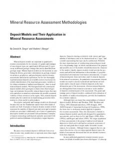
CEA used the Cast3m tool [4] which allows solving flow equation (5) and transport equation (4) using Finite Volume and Mixed Hybrid Finite Element spatial schemes. The Cast3m tool also allows using different type of solvers ranging from direct solver to multi-grid solver and including conjugate gradient solvers. The CEA contribution includes 1D, 2D and 3D calculations with both rectangular and cylindrical description for all selected radionuclides except for the decay chain. Calculations were performed using different level of mesh refinement. An example of meshes used is presented on Figure 7.
(a) (b)
(c)
(d)
(e)
(f)
Figure 7: Coarser refined meshes used (the host rock is blue). (a) 1D cylindrical shape (18 cells), (b) 1D cubic shape (18 cells), (c) 2D cylindrical shape (34 cells), (d) 2D cubic shape (126 cells), (e) 3D cylindrical shape (5536 cells), (f) 3D cubic shape (8640 cells).
PAMINA Sixth Framework programme, 14.10.2009
19
Code and meshes used by IRSN IRSN used a commercial code, GoldSim, and the Melodie software, which is a numerical tool developed by IRSN in collaboration with the Paris School of Mines to model the transport of radionuclides in the context of radioactive waste disposal. The initial design of the Melodie software was based on Finite Element (FE) method for numerical approximation of flow (1) and transport (2) equations. The FE method, commonly used to solve parabolic and elliptical problems, is not satisfactory for dealing with possible discontinuities in calculation results and with advection terms, especially when the advection is predominant compared to diffusion. To improve the accuracy and the reliability of calculations, a method called Finite Volume Finite Element (FVFE) has been adapted in Melodie. Using 3D models, FVFE method operates on tetrahedral elements and requires constructing a dual mesh. In the modeling case, the dual mesh is based on centres of gravity. A first mesh has thus been built using tetrahedral elements fulfilling the dihedron angle criterion. FE method has been tested on the same tetrahedral mesh, as well as on a hexahedral mesh. The tetrahedral mesh is composed of 80,199 computational nodes and 443,520 elements and a hexahedral mesh is composed of 80,199 nodes and 73,920 elements (Figure 8). GoldSim code was used to simplify the phenomenological 3D modelling into a compartmental modelling (not presented in that document). GoldSim is a general purpose simulation environment with an integrated graphical user interface for modelling and data output. A contaminant transport module provides the ability to simulate the transport and fate of radionuclides through the environment (e.g. for performance assessment).
PAMINA Sixth Framework programme, 14.10.2009
20
(a)
(b)
(c) (d) Figure 8: Tetrahedral ((a) tunnel axe and (b) longitudinal views) and hexahedral ((c) tunnel axe and (d) longitudinal views) meshes.
PAMINA Sixth Framework programme, 14.10.2009
21
Code and meshes used by SCK-CEN SCK•CEN used two commercial codes. The first one based on Finite Volume spatial scheme was PORFLOW 3.07 [6] and the second one based on Finite Element spatial scheme was COMSOL Multiphysics 3.2 (earth science module) [2]. The SCK•CEN contribution so far includes 1D and 2D calculations with a rectangular gallery approximation, using a FE method (COMSOL multiphysics [2]) and a FV code (PORFLOW 3.07 [6]). An example of the grids used in the calculations is shown in Figure 9. 50
obs2
obs2 45
40
35
30
25
20
15
10
5
obs1
obs1 0 0
5
10
Figure 9: Example of grid spacing used with PORFLOW (left) and FE mesh used with COMSOL multiphysics (right) (zoom on the upper half of the model domain), and position of observation nodes. As output parameters, SCK•CEN systematically recorded the instantaneous radionuclide flux to the overlying aquifer, the concentration in the source zone (obs1 in Figure 9), and the concentration in the clay in close proximity of the overlying aquifer (obs2 in Figure 9).
PAMINA Sixth Framework programme, 14.10.2009
22
5.2
Flow calculation results
Flow calculations were performed by CEA, IRSN and SCK-CEN on each domain dimensionality and geometry described previously. CEA flow calculation results: CEA used different meshes of increasing level of refinement as well as Finite Volume and Mixed Hybrid Finite Element spatial scheme. No noticeable impact of refinement nether spatial numerical scheme was found concerning flow calculation results. An example of calculated heads results for cubic shape (Finite volume, 1D, 2D and 3D) are presented on Figure 10. MIN−MAX >3.50E+02 3.50E+02 3.52E+02