Parallel approximation of min-max problems

Parallel approximation of min-max problems Gus Gutoski∗ ∗

Institute for Quantum Computing and School of Computer Science University of Waterloo, Waterloo, Ontario, Canada †

arXiv:1011.2787v3 [quant-ph] 8 Dec 2012

Xiaodi Wu†

Department of Electrical Engineering and Computer Science University of Michigan, Ann Arbor, Michigan, USA

December 7, 2012 Abstract This paper presents an efficient parallel approximation scheme for a new class of min-max problems. The algorithm is derived from the matrix multiplicative weights update method and can be used to find near-optimal strategies for competitive two-party classical or quantum interactions in which a referee exchanges any number of messages with one party followed by any number of additional messages with the other. It considerably extends the class of interactions which admit parallel solutions, demonstrating for the first time the existence of a parallel algorithm for an interaction in which one party reacts adaptively to the other. As a consequence, we prove that several competing-provers complexity classes collapse to PSPACE such as QRG(2), SQG and two new classes called DIP and DQIP. A special case of our result is a parallel approximation scheme for a specific class of semidefinite programs whose feasible region consists of lists of semidefinite matrices that satisfy a transcript-like consistency condition. Applied to this special case, our algorithm yields a direct polynomial-space simulation of multi-message quantum interactive proofs resulting in a first-principles proof of QIP = PSPACE.

1

Introduction

This paper presents a parallel approximation scheme for a new class of min-max problems with applications to classical and quantum zero-sum games and interactive proofs. In order to describe this class of min-max problems let us begin by considering a semidefinite program (SDP) of the form minimize

Tr(Xk P )

subject to

TrMn (Xi+1 ) = Φi (Xi ) for i = 1, . . . , k − 1

Tr(X1 ) = 1

(1)

0  X1 , . . . , Xk ∈ Mmn Here Md denotes the space of all d × d complex matrices and TrMn is the partial trace—the unique linear map from matrices to matrices satisfying TrMn : Mmn → Mm : A ⊗ B 7→ Tr(B)A for every choice of A ∈ Mm and B ∈ Mn . An SDP (1) is specified by arbitrary choices of a positive semidefinite matrix P ∈ Mmn with kP k ≤ 1 and completely positive and trace-preserving linear maps 1

Φ1 , . . . , Φk−1 : Mmn → Mm . (A linear map Φ is positive if Φ(X)  0 whenever X  0. Such a map is completely positive if Φ ⊗ 1Md is positive for every positive integer d.) Let A denote the feasible region of the SDP (1) (which is always non-empty) and let P ⊂ Mmn be a non-empty compact convex subset of positive semidefinite matrices having operator norm at most 1. We are concerned with the following min-max problem, which is a generalization of the SDP (1): def

λ(A, P) =

min

max Tr(Xk P )

(X1 ,...,Xk )∈A P ∈P

(2)

The ordering of minimization and maximization is immaterial, as implied by well-known extensions of von Neumann’s Min-Max Theorem [vN28, Fan53] given the fact that A, P are convex compact sets and Tr(Xk P ) is a bilinear form over the two sets. Our main result is an efficient parallel oracle-algorithm for finding approximate solutions to the minmax problem (2) and for approximating the quantity λ(A, P), given an oracle for optimization over the set P. We also describe parallel implementations of this oracle for certain sets P, yielding an unconditionally efficient parallel approximation scheme for the min-max problem (2) for those choices of P. This result is stated formally below as Theorem 1. Before stating this theorem let us clarify terminology.

1.1

Review of parallel computation, formal statement of results

Recall that a parallel algorithm is described by a family of logarithmic-space uniform Boolean circuits. The uniformity constraint ensures that the size of each circuit in the family scales as a polynomial in the bit length of the input, and therefore the family represents a polynomial-time computation. Boolean circuits are an ideal model of parallel computation because computational activity can occur concurrently at many different gates in the circuit. Indeed, the run time of a parallel algorithm is determined by the depth of its circuits, which might be much smaller than the total size of its circuits. A parallel algorithm is said to be efficient if the depth of its circuits (and therefore the run time of the algorithm) scales as a polynomial in the logarithm of the bit length of the input. The complexity class NC consists of those functions which can be computed by efficient parallel algorithms. Efficient parallel algorithms are sometimes called “NC algorithms” or “NC computations.” The reader is referred to [Pap94] for an accessible introduction to parallel computation. An oracle-algorithm is an algorithm endowed with the ability to get instantaneous answers to questions that fall within the scope of some specific oracle. In our case, we assume an oracle for optimization over P, which instantly solves problems of the form Problem 1 (Optimization over P). Input: A matrix X  0 with Tr(X) = 1 and an accuracy parameter δ > 0. Output:

A near-optimal element P ? ∈ P such that Tr(XP ? ) ≥ Tr(XP ) − δ for all P ∈ P.

An oracle is incorporated into the circuit model of computation by supplementing a standard gate set (such as {AND, OR, NOT}) with a special oracle gate. This oracle gate has many input bits (describing the question) and many output bits (describing the answer). As with standard gates, each oracle gate contributes unit cost to circuit size and run time. An approximation scheme refers to an algorithm that computes one or more quantities to a given precision δ and whose run time is efficient for each fixed choice of δ > 0 but does not necessarily scale well with δ. In the circuit model (and other models, too) this property is encapsulated by defining the underlying problem so that the accuracy parameter δ = 1/s is specified in unary as 1s , thus forcing the bit length of the 2

input to be proportional to 1/δ instead of 1/ log(δ). The choice to specify the accuracy parameter in unary allows parallel approximation schemes to be described neatly by log-space uniform circuits with polylog depth. The following is a formal statement of the problem solved by our algorithm. Problem 2 (Approximation of λ(A, P)). Input: Completely positive and trace-preserving linear maps Φ1 , . . . , Φk−1 specifying the feasible region A of an SDP of the form (1). An accuracy parameter δ > 0. Oracle:

Optimization over P (Problem 1).

Output:

Near-optimal elements (X1? , . . . , Xk? ) ∈ A and P ? ∈ P such that Tr(Xk? P ) ≤ λ(A, P) + δ for all P ∈ P

Tr(Xk P ? ) ≥ λ(A, P) − δ for all (X1 , . . . , Xk ) ∈ A ˜ with | λ ˜ − λ(A, P)| ≤ δ. and a quantity λ The maps Φ1 , . . . , Φk−1 are linear maps from a complex vector space of dimension (mn)2 to another complex space of dimension m2 . As such, these maps can be represented by complex matrices of size m2 × (mn)2 . In both Problem 1 and Problem 2 it is assumed that the real and imaginary parts of each entry in each input matrix are represented as rational numbers expressed as the ratio of two p-bit integers written in binary for some p that is promised to scale as a polynomial in the dimension mn. (Indeed, it suffices for our purpose that p scales logarithmically with mn.) As suggested previously, it is also assumed that the accuracy parameter δ is represented in unary. These assumptions allow us to focus on the quantities mn, k, 1/δ as the dominating factors determining the run time of our parallel algorithm. We may now state our main result. Theorem 1 (Main result). There is a parallel oracle-algorithm for Problem 2 (Approximation of λ(A, P)) with run time bounded by a polynomial in k, 1/δ, and log(mn). This algorithm is efficient if k, 1/δ are promised to scale as a polynomial in log(mn).

1.2

Application: parallel approximation of semidefinite programs

The SDP (1) is recovered from (2) in the special case where P = {P } is a singleton set. Thus, a special case of Theorem 1 is a parallel approximation scheme for SDPs of the form (1). We restricted attention to SDPs for which kP k, Tr(X1 ) ≤ 1 because this restriction does not interfere with our application to quantum interactive protocols and because the run time of our parallel algorithm scales polynomially with the largest eigenvalue of P and with the trace of X1 , so it is only efficient when these quantities are bounded by a fixed polynomial in the logarithm of the bit length of the input P, Φ1 , . . . , Φk−1 . (In keeping with convention, one can think of these quantities as the width of the SDPs we consider. Our algorithm is efficient only for width-bounded SDPs.) It has long since been known that the problem of approximating the optimal value of an arbitrary SDP is logspace-hard for P [Ser91, Meg92], so there cannot be a parallel approximation scheme for all SDPs unless NC = P. The precise extent to which SDPs admit parallel solutions is not known. This special case of our result adds considerably to the set of such SDPs, subsuming all prior work in the area at the time it was made public. (Since that time parallel approximation schemes have been found for some SDPs of unbounded width that are not covered by our scheme [JY11, PT12, JY12].) 3

Some of what is known about SDPs in this respect is inherited knowledge from linear programs (LPs). For example, Luby and Nisan describe a parallel approximation scheme for so-called positive LPs of the form minimize xp∗ subject to Cx ≥ q and x ≥ 0 where each entry of the matrix C and vectors p, q is a nonnegative real number [LN93]. Young provides a generalization of Luby-Nisan to arbitrary mixed packing and covering problems [You01]. By contrast, Trevisan and Xhafa show that it is P-hard to find exact solutions for positive LPs [TX98].1 The notion of a positive instance of an LP can be generalized to SDPs as follows. An SDP of the form minimize Tr(XP ) subject to Ψ(X)  Q and X  0 is said to be positive if P, Q  0 and Ψ is a positive map. Of course, P-hardness of exact solutions for positive LPs implies P-hardness of exact solutions for positive SDPs. Jain and Watrous give a parallel approximation scheme for width-bounded positive SDPs [JW09]. Subsequent improvements extend to all positive SDPs [JY11, PT12], and even to mixed packing and covering SDPs [JY12]. The Jain-Watrous algorithm for positive SDPs is derived from a correspondence between positive SDPs and one-turn quantum games and can therefore be recovered as a special case of the work of the present paper. In their proof of QIP = PSPACE, Jain et al. give a parallel algorithm for a specific SDP based on quantum interactive proofs [JJUW11]. It is not difficult to see that their SDP can be written in the form (1) considered in the present paper. As mentioned above, our algorithm is not efficient when used for SDPs of unbounded width, leaving the recent works of Jain and Yao [JY11, JY12] and Peng and Tangwongsan [PT12] on mixed packing and covering SDPs as the only known parallel SDP approximation schemes that are not subsumed by the present work. These recent works do not subsume our results, as neither the SDP instance used in Ref. [JJUW11] to prove QIP = PSPACE nor its generalization (1) in the present paper are mixed packing and covering SDPs.

1.3 1.3.1

Application: interactive proofs with competing provers Definitions

An interactive proof with competing provers consists of a conversation between a verifier and two provers regarding some input string x. The verifier may use randomness, but must run in time that scales as a polynomial in the input length |x|; the provers are permitted unlimited computational power. One of the provers—the yes-prover—tries to convince the verifier to accept x, while the other—the no-prover—tries to convince the verifier to reject x. A decision problem L is said to admit an interactive proof with competing provers with completeness c and soundness s if there exists c, s with c > s and a randomized polynomialtime verifier who meets the following conditions: Completeness condition. If x is a yes-instance of L then the yes-prover can convince the verifier to accept with probability at least c regardless of the no-prover’s strategy. Soundness condition. If x is a no-instance of L then the no-prover can convince the verifier to reject with probability at least 1 − s regardless of the yes-prover’s strategy. 1 For clarification, a polynomial-time algorithm finds an exact solution to an LP or SDP if it finds solutions that are within ε of optimal in time polynomial in the bit length of ε—that is, log(1/ε). By contrast, an approximation scheme for LPs or SDPs finds solutions that are within ε of optimal with run time that depends super-polynomially in the bit length of ε—typically 1/ε.

4

The completeness and soundness parameters c, s need not be fixed constants, but may instead vary as a function of the input length |x|. If these parameters are not specified then it is assumed that L admits an interactive proof with competing provers for some choice of c(|x|), s(|x|) for which there exists a polynomial-bounded function p(|x|) such that c − s ≥ 1/p. The complexity class RG consists of all decision problems that admit interactive proofs with competing provers. (The acronym RG stands for “refereed games,” a term inspired by the field of game theory). Often in the study of interactive proofs the precise values of c, s are immaterial because sequential repetition (or sometimes parallel repetition) can be used to transform any verifier for which c − s ≥ 1/p into another verifier for which c tends toward one and s tends toward zero exponentially quickly in the bit length of x. (For example, sequential repetition followed by a majority vote can be used to reduce error for RG.) For this reason, it is typical to assume without loss of generality that c, s are constants such as 2/3, 1/3 or that c is exponentially close to one and s is exponentially close to zero whenever it is convenient to do so. However, it is not always clear that a given complexity class is robust with respect to the choice of c, s so it is good practice to be as inclusive as possible when defining these classes. Interesting subclasses of RG are obtained by placing restrictions upon the number and timing of messages in the interaction between the verifier and provers. In this paper we introduce one such subclass based upon interactions of the following form: 1. The verifier exchanges several messages with only the yes-prover. 2. After processing this interaction with the yes-prover, the verifier exchanges several additional messages with only the no-prover. 3. After further processing, the referee declares acceptance or rejection. Interactive proofs of this form shall be called double interactive proofs: the verifier in such a protocol executes a standard single-prover interactive proof with the yes-prover followed by a second single-prover interactive proof with the no-prover. The class of problems that admit double interactive proofs shall be called DIP. By contrast to RG, it is not immediately clear that the definition of DIP is robust with respect to the choice of parameters c, s. But it follows from our result that DIP is, in fact, robust with respect to the choice of c, s. Also, whereas RG is trivially closed under complement, the protocol for double interactive proofs is asymmetric and so it is not immediately clear that DIP is closed under complement. Again, it follows from our result that DIP is closed under complement. Another example of an interesting subclass of RG is the family of bounded-turn classes. For each positive integer k the class RG(k) consists of those problems that admit an interactive proof with competing provers in which the verifier exchanges no more than k messages with each prover. It is understood that messages are exchanged with the provers in parallel so that RG(k), like RG, is trivially closed under complement. Quantum interactive proofs with competing provers are defined similarly except that the verifier is a polynomial-time quantum computer who exchanges quantum information with the provers. The analogous complexity classes are denoted QRG, DQIP, and QRG(k). 1.3.2

Prior work

As noted in Refs. [FKS95, FK97], the results of Koller and Meggido [KM92] and Koller, Megiddo, and von Stengel [KMvS94] imply that RG ⊆ EXP. The reverse containment was proven by Feige and Kilian 5

[FK97], yielding the characterization RG = EXP. It was proven in Ref. [GW07] that QRG ⊆ EXP, from which one obtains QRG = RG = EXP, which is the competing-provers version of the well-known collapse QIP = IP = PSPACE for singleprover interactive proofs [LFKN92, Sha92, JJUW11]. For bounded-turn classes, the results of Fortnow et al. tell us that RG(1) is essentially a randomized 2 version of SP 2 [FIKU08]. Feige and Kilian proved RG(2) = PSPACE [FK97]. For bounded-turn quantum classes, [JW09] proved QRG(1) ⊆ PSPACE. The complexity of QRG(2) is an open question of [JJUW11] that is solved in the present paper. The exact complexity of RG(k) and QRG(k) for all other k is not known. Bounded-turn double quantum interactive proofs have been studied previously under the name short quantum games; the associated complexity class has been called SQG. In an effort to unify notation let DQIP(k, l) denote the class consisting of problems that admit a double quantum interactive proof with competing provers in which the verifier exchanges no more than k messages with the yes-prover followed by no more than l messages with the no-prover. The class SQG was first defined in Ref. [GW05] to be equal to DQIP(1, 2), wherein it was shown that this class contains QIP = DQIP(poly, 0). The importance of short quantum games has been diminished by the proof of QIP = PSPACE, as containment of QIP is no longer such a peculiar property. However, the containment of PSPACE inside DQIP(1, 2) is still interesting, as it is not known whether PSPACE is contained in DIP(1, 2), the classical version of this class. 1.3.3

Our contribution

As we explain in Section 5, the oracle-algorithm of Theorem 1—together with a parallel implementation of a suitably chosen oracle—implies that near-optimal strategies for the provers in a double quantum interactive proof can be computed efficiently in parallel. The following containment then follows from a standard argument (summarized in Section 5.4). Theorem 2. DQIP ⊆ PSPACE. This containment, when combined with the trivial containments IP ⊆ DIP ⊆ DQIP and the wellknown fact that PSPACE ⊆ IP [LFKN92, Sha92], yields the following characterization. Corollary 2.1. DQIP = DIP = PSPACE. As a special case of Corollary 2.1 we obtain the solution to an open problem of [JJUW11]: Corollary 2.2. QRG(2) = PSPACE. Another special case of our result is a direct polynomial-space simulation of multi-message quantum interactive proofs, resulting in a first-principles proof of QIP = PSPACE. Corollary 2.3. QIP = PSPACE via direct polynomial-space simulation of multi-message quantum interactive proofs. 2

The class we call RG(2) is called RG(1) by Feige and Kilian [FK97]. This conflict in notation stems from the fact that we measure the length of an interaction in turns (i.e. messages per prover), whereas those authors measure an interaction in rounds of messages. This switch of notation was instigated by Jain and Watrous, who required a convenient symbol for one-turn interactions [JW09].

6

By contrast, all other known proofs [JJUW11, Wu10] rely upon the fact that the verifier can be assumed to exchange only three messages with the prover [KW00]. The original proof of Jain et al. [JJUW11] also relies on the additional fact that the verifier’s only message to the prover can be just a single classical coin flip [MW05]. Of course, every other competing-provers complexity class whose protocol can be cast as a double interactive proof also collapses to PSPACE, such as the aforementioned class DQIP(1, 2) based on short quantum games. It follows from the collapse of DQIP and DIP to PSPACE that these classes are closed under complement and that they are robust with respect to the choice of parameters c, s. (Indeed, it may be assumed that c = 1 and s ≤ 2−q for any desired polynomially-bounded function q(|x|)—see Section 6.3.) Prior to the present work polynomial-space algorithms were known only for two-turn classical interactive proofs with competing provers (RG(2)), for one-turn quantum interactive proofs with competing provers (QRG(1)), and for single-prover quantum interactive proofs (QIP). Our result unifies and subsumes all of these algorithms. It also demonstrates for the first time the existence of a polynomial-space algorithm for a competing-prover interaction (classical or quantum) in which one prover reacts adaptively to the other. Finally, our results illustrate a difference in the effect of public randomness between single-prover interactive proofs and competing-prover interactive proofs. Any classical interactive proof with single prover can be simulated by another public-coin interactive proof where the verifier’s messages to the prover consist entirely of uniformly random bits and the verifier uses no other randomness [GS89]. Extending the notion of public-coin interaction to competing-prover interactions, it is easy to see that any such interaction with a public-coin verifier can be simulated by a double interactive proof.3 We therefore have that the public-coin version of RG is a subset of DIP, which we now know is equal to PSPACE. Thus, by contrast to the single-prover case where public-coin-IP = IP, in the competing-prover case we establish the following. Corollary 2.4. public-coin-RG 6= RG unless PSPACE = EXP.

1.4 1.4.1

Summary of techniques The matrix multiplicative weights update method

The parallel oracle-algorithm we exhibit in the proof of Theorem 1 is an example of the matrix multiplicative weights update method (MMW) as presented in Refs. [AHK05, WK06, Kal07]. We draw upon the valuable experience of recent applications of this method to parallel algorithms for quantum complexity classes [JW09, JUW09, JJUW11, Wu10]. We also make extensive use of efficient parallel algorithms for various matrix manipulation tasks, such as computing the singular value decomposition or exponential of a matrix. The reader is referred to von zur Gathen for more detail on parallel algorithms for matrix operations [vzG93] and to works of Jain et al. for discussion of the use of these algorithms in parallel implementations of the matrix multiplicative weights update method [JUW09, JJUW11]. In its unaltered form, the MMW can be used to solve min-max problems over the domain of density operators—positive semidefinite matrices X with Tr(X) = 1. We introduce a new extension to this method for min-max problems over the domain A defined in the SDP (1)—a domain consisting of k-tuples of density operators lying within a strict subspace of the affine space associated with k-tuples of density operators. The high-level approach of our method is as follows: 3 Proof sketch: As the verifiers’s questions to each prover are uniformly random, they cannot depend on prior responses from the other prover and can therefore be reordered so that all messages with one prover are exchanged before any messages with the other.

7

1. Extend the domain from a single density matrix to a k-tuple of density matrices. This step is straightforward: the MMW can be applied without complication to all k density matrices at the same time. (Equivalently, k density matrices may be viewed as a single, larger, block-diagonal density matrix.) 2. Restrict the domain to a strict subspace of k-tuples of density matrices. This step is more difficult. It is accomplished by relaxing the problem so as to allow all k-tuples, with an additional penalty term to remove incentive for the players to use inconsistent transcripts. 3. Round strategies in the relaxed problem to strategies in the original protocol. For this step one must prove a “rounding” theorem (Theorem 5), which establishes that near-optimal, fully admissible strategies can be obtained from near-optimal strategies in the unrestricted domain with penalty term. 1.4.2

Finding optimal strategies for the provers in a double quantum interactive proof

In Section 5 we observe that the verifier in a double quantum interactive proof induces a min-max problem of the form (2) in which elements of A correspond to strategies for the yes-prover and elements of P correspond to strategies for the no-prover. Thus, the parallel oracle-algorithm of Theorem 1—together with a parallel implementation of the oracle for optimization over P—can be used to find optimal strategies for the provers in a double quantum interactive proof. Our implementation of this oracle is itself a special case of the algorithm of Theorem 1, so that the overall algorithm employs the MMW method twice in a two-level recursive fashion. At the top level the MMW is used to iteratively converge toward an optimal strategy for the yes-prover; at the bottom level the MMW is used again to solve an SDP for “best responses” for the no-prover to a given strategy for the yes-prover. The central challenge in using the MMW to find optimal strategies for parties in a quantum interaction is to find a representation for strategies that is amenable to the MMW method. In Kitaev’s transcript representation [Kit02] the actions of a prover in a double quantum interactive proof are represented by a list X1 , . . . , Xk of density matrices that satisfy a special consistency condition that is captured by the definition of the feasible region A of the SDP (1). Intuitively, these density matrices correspond to “snapshots” of the state of the verifier’s qubits at various times during the interaction. (See Figure 3 on page 20.) The key property of double quantum interactive proofs that we exploit is the ability to draw a “temporal line” in the interaction before which only the yes-prover acts and after which only the no-prover acts. Given a transcript X1 , . . . , Xk for the yes-prover, the actions of the no-prover can then be represented by another transcript Y1 , . . . , Y` . By optimizing over all such transcripts one obtains an oracle for “best responses” for the no-prover to a given strategy of the yes-prover as required by the MMW method. 1.4.3

Comparison of methods for semidefinite programming

In their proof of QIP = PSPACE, Jain et al. [JJUW11] employ the MMW to solve a special SDP for quantum interactive proofs by making direct use of the primal-dual approach described in Kale’s thesis [Kal07]. Subsequent parallel algorithms for positive SDPs [JY11, PT12] and for mixed packing and covering SDPs [JY12] are matrix generalizations (also based on MMW) of existing algorithms for linear programs [LN93, You01]. We do not use any of these approaches for solving SDPs. Instead we use the MMW to solve a min-max problem as suggested by the algorithmic proof (also presented in Kale’s thesis) of a min-max theorem for 8

a simple class of zero-sum quantum games. By introducing a penalty term for inadmissible strategies we are able to extend this algorithm to a much richer class of games beyond the one-turn games considered by Kale. We wish to stress that our parallel algorithm for SDPs arises as a special case of a more general min-max algorithm, whereas previous approaches for SDPs do not generalize to min-max problems in any obvious way. 1.4.4

Comparison of proofs of QIP = PSPACE

Unlike the present paper, the original proof of QIP = PSPACE due to Jain et al. [JJUW11] does not take advantage of the transcript representation for arbitrary multi-turn strategies. Instead, as mentioned earlier, those authors derive a special SDP by invoking several nontrivial facts about quantum interactive proofs. Admittedly, their SDP does bear a resemblance to Kitaev’s transcript conditions, but this resemblance is only superficial and their solution applies only to a very restricted subset of transcripts. Indeed, their derivation breaks down without the assumption that the verifier sends only classical messages to the prover. Previously one of us [Wu10] presented a simplified proof of QIP = PSPACE that, like the work of the present paper, employs Kale’s algorithmic min-max theorem [Kal07] instead of the primal-dual approach for SDPs that was used in the original proof by Jain et al. [JJUW11]. The QIP-completeness of the quantum circuit distinguishability problem [RW05] means that quantum interactive proofs can be decided by approximating the diamond norm of the difference between two quantum channels. Wu noticed that the diamond norm can be approximated in this special case by a direct application of Kale’s algorithmic min-max theorem. His result did not require the penalization method introduced in the present paper nor an attendant rounding theorem. 1.4.5

The Bures angle

Finally, it is noteworthy that the proof of our rounding theorem (Theorem 5) contains an interesting and nontrivial application of the Bures angle, which is a distance measure for quantum states that is defined in terms of the more familiar fidelity function. Properties of the trace norm, which captures the physical distinguishability of quantum states, are sufficient for most needs in quantum information. When some property of the fidelity is also required one uses the Fuchs-van de Graaf inequalities to convert between the trace norm and fidelity [FvdG99]. (These inequalities are listed in Eq. (4) of Section 2.3.) However, every such conversion incurs a quadratic slackening of relevant accuracy parameters. Our study calls for repeated conversions, which would incur an unacceptable exponential slackening if done naively via Fuchs-van de Graaf. Instead, we make only a single conversion between the trace norm and the Bures angle and then repeatedly exploit the simultaneous properties of (i) the triangle inequality, (ii) contractivity under quantum channels, and (iii) preservation of subsystem fidelity. Although conversion inequalities between the trace norm and Bures metric are implied by Fuchs-van de Graaf, to our knowledge explicit conversion inequalities have not yet appeared in published literature. The required inequalities are derived in the present paper (Proposition 4).

2

Preliminaries

Hereafter we must assume familiarity with standard concepts from quantum information, though we have attempted to minimize our use of quantum formalism for the benefit of a wider audience. The reader is referred to Nielsen and Chuang [NC00] and to the lecture notes of Watrous [Wat11] for proper introductions 9

to the field. This section provides a short glossary clarifying our notation and terminology in Section 2.1 followed by a review of two rarer but nonetheless simple and fundamental concepts from quantum information: the preservation of subsystem fidelity in Section 2.2 and the Bures angle in Section 2.3.

2.1

Terminology and notation

Density matrix, quantum state. A density matrix or quantum state is a positive semidefinite matrix X with Tr(X) = 1. Thus far, we have used upper-case Roman letters (X, Y, . . . ) to denote density matrices, as well as other matrices. But it is standard practice in quantum information to denote density matrices with lower-case Greek letters (ρ, ξ, . . . ). Hereafter we adopt this convention. Measurement operator. A measurement operator is a positive semidefinite matrix M with kM k ≤ 1. Equivalently, it holds that 0  M  I. Quantum channel. A channel is a completely positive and trace-preserving linear map Φ : Mm → Mn from matrices to matrices. These maps correspond to physically realizable operations on quantum states. Adjoint, matrix inner product. The adjoint A∗ of a matrix A is simply the conjugate-transpose of A. The inner product hA, Bi between two m × n matrices A, B is given by hA, Bi = Tr(A∗ B). The inner product between two k-tuples of matrices is given by the sum h(A1 , . . . , Ak ), (B1 , . . . , Bk )i =

k X i=1

hAi , Bi i.

Φ∗

More generally, the adjoint of a linear map Φ from matrices to matrices is the unique linear map with hΦ(X), Y i = hX, Φ∗ (Y )i for all X, Y . This formula extends in the obvious way to linear maps from tuples of matrices to tuples of matrices. Trace norm. The trace norm kX kTr of a matrix X is defined as the sum of the singular values of X. As a measure of distance between quantum states, the trace norm is given by 1 kρ − ξ kTr = max hρ − ξ, Πi 0ΠI 2

(3)

for all density matrices ρ, ξ. Fidelity. The fidelity is another distance measure for quantum states given by

√ p

F (ρ, ξ) = ρ ξ Tr

for all density matrices ρ, ξ.

2.2

Preservation of subsystem fidelity

Consider the following property of the fidelity function, which we call the preservation of subsystem fidelity: if ρ, ξ are states of a quantum system with fidelity F (ρ, ξ) and ρ0 is any state of a larger system consistent with ρ then it is always possible to find ξ 0 consistent with ξ such that F (ρ0 , ξ 0 ) = F (ρ, ξ). A formal construction of such a ξ 0 appears in Ref. [JUW09]. Since their construction consists entirely of elementary matrix operations, there is an efficient parallel algorithm that takes as input ρ, ξ, ρ0 and produces the desired state ξ 0 as output. 10

Proposition 3 (Preservation of subsystem fidelity [JUW09, Lemma 7.2]). Let ρ, ξ ∈ Mm and ρ0 ∈ Mmn be density matrices with TrMn (ρ0 ) = ρ. There exists a density matrix ξ 0 ∈ Mmn with TrMm (ξ 0 ) = ξ and F (ρ0 , ξ 0 ) = F (ρ, ξ). Moreover ξ 0 can be computed efficiently in parallel given ρ, ξ, ρ0 .

2.3

The Bures angle

The Bures angle or simply the angle A(ρ, ξ) between quantum states ρ, ξ is defined by def

A(ρ, ξ) = arccos F (ρ, ξ). The angle is a metric on quantum states, meaning that it is nonnegative, equals zero only when ρ = ξ, and obeys the triangle inequality [NC00]. Moreover, the angle is contractive, so that A(Φ(ρ), Φ(ξ)) ≤ A(ρ, ξ) for any quantum channel Φ. The Fuchs-van de Graaf inequalities establish a relationship between the fidelity and trace norm [FvdG99]. The inequalities are p 1 1 − F (ρ, ξ) ≤ kρ − ξ kTr ≤ 1 − F (ρ, ξ)2 . 2

(4)

These inequalities can be used to derive a relationship between A(ρ, ξ) and kρ − ξ kTr . For example, Proposition 4 (Relationship between trace norm and Bures angle). For all density matrices ρ, ξ it holds that r 1 π kρ − ξ kTr ≤ A(ρ, ξ) ≤ kρ − ξ kTr . 2 2 Proof. The lower bound on A(ρ, ξ) follows immediately from Fuchs-van de Graaf: p 1 kρ − ξ kTr ≤ 1 − cos A(ρ, ξ)2 = sin A(ρ, ξ) ≤ A(ρ, ξ) 2 where we used the identity sin x ≤ x for all x ≥ 0. To obtain the upper bound on A(ρ, ξ) we employ the identity cos x ≤ 1 − x2 /π for x ∈ [0, π/2], which can be verified using basic calculus. Then we have 1 A(ρ, ξ)2 kρ − ξ kTr ≥ 1 − cos A(ρ, ξ) ≥ 2 π from which the proposition follows.

3

Rounding theorem for a relaxed min-max problem

In this section we define a new min-max expression µε (A, P) that approximates the desired quantity λ(A, P) from (2) in the limit as ε approaches zero. This new expression is a relaxation of λ(A, P) that is more amenable to the MMW. We prove a “rounding theorem” (Theorem 5) by which near-optimal points for λ(A, P) are efficiently obtained from near-optimal points for µε (A, P). Our use of the Bures angle occurs in the proof of Lemma 8, which is used in the proof of our rounding theorem.

11

Define the relaxation µε (A, P) of λ(A, P) by def

µε (A, P) =

=

min

(ρ1 ,...,ρk )

max

P ∈P (Π1 ,...,Πk−1 )

k−1 kX hρk , P i + hTrMn (ρi+1 ) − Φi (ρi ), Πi i ε i=1

min max hρk , P i +

(ρ1 ,...,ρk ) P ∈P

k−1 kX1 kTrMn (ρi+1 ) − Φi (ρi )kTr ε 2 i=1

Here the minimum is taken over all density operators ρ1 , . . . , ρk ∈ Mmn and the maximum over all P ∈ P and over all measurement operators Π1 , . . . , Πk−1 ∈ Mm . The second equality follows immediately from the identity (3) from Section 2.1. Notice that the minimum in the definition of µε (A, P) is taken over all k-tuples (ρ1 , . . . , ρk ) of density operators, not just those in A. Each term in the summation serves to penalize any violation of the conditions required for membership in A by adding the magnitude of that violation to the objective function. The k/ε factor amplifies the penalty so as to remove incentive to select an element outside of A. Indeed, it is clear that lim µε (A, P) = λ(A, P). ε→0

The following “rounding” theorem establishes a specific rate of convergence for this limit. A subsequent extension of this theorem (Proposition 7) provides a means by which near-optimal points for λ(A, P) are efficiently computed from near-optimal points for µε (A, P). Theorem 5 (Rounding theorem). For any ε > 0 it holds that λ(A, P) ≥ µε (A, P) > λ(A, P) − ε. Proof. The first inequality is easy: let (ρ1 , . . . , ρk ) be optimal for λ(A, P) and let (P, Π1 , . . . , Πk−1 ) be optimal for µε (A, P). Then we have λ(A, P) ≥ hρk , P i = hρk , P i +

k−1 kX hTrMn (ρi+1 ) − Φi (ρi ), Πi i ≥ µε (A, P). ε i=1

(The first inequality is because (ρ1 , . . . , ρk ) is optimal for λ(A, P). The equality follows because (ρ1 , . . . , ρk ) ∈ A, so each term in the sum is zero. The final inequality is because (P, Π1 , . . . , Πk−1 ) is optimal for µε (A, P).) The second inequality is more difficult. We invoke the following lemma, the proof of which appears later in this section. Lemma 6 (Rounding lemma). For any ε > 0 and any states ρ1 , . . . , ρk ∈ Mmn there exists (ρ01 , . . . , ρ0k ) ∈ A such that k−1 1 kX1 0 kρk − ρk kTr < ε + kTrMn (ρi+1 ) − Φi (ρi )kTr . 2 ε 2 i=1

Moreover,

ρ01 , . . . , ρ0k

can be computed efficiently in parallel given ρ1 , . . . , ρk .

Let (ρ1 , . . . , ρk ) be optimal for µε (A, P), let (ρ01 , . . . , ρ0k ) be the density operators obtained by invoking Lemma 6, and let P ∈ P be optimal for λ(A, P). Because (ρ1 , . . . , ρk ) is optimal for µε (A, P) we have µε (A, P) ≥ hρk , P i +

k−1 kX1 kTrMn (ρi+1 ) − Φi (ρi )kTr ε 2 i=1

12

(5)

Employing the identity (3), the quantity hρk , P i becomes





 1 hρk , P i = ρ0k , P + ρk − ρ0k , P ≥ ρ0k , P − ρk − ρ0k Tr . 2 Substituting the bound on is canceled, leaving

1 2

kρk − ρ0k kTr from Lemma 6, we see that the summation of trace norms in (5)

 µε (A, P) > ρ0k , P − ε ≥ λ(A, P) − ε

as desired. (The final inequality is because P is optimal for λ(A, P).) Proposition 7 (Construction of near-optimal strategies). The following hold for any δ, ε > 0: 1. If (ρ1 , . . . , ρk ) is δ-optimal for µε (A, P) then there is an efficient parallel algorithm to compute (ρ01 , . . . , ρ0k ) ∈ A that is (δ + ε)-optimal for λ(A, P). 2. If (P, Π1 , . . . , Πk−1 ) is δ-optimal for µε (A, P) then P is also (δ + ε)-optimal for λ(A, P). Proof of item 1. Let (ρ1 , . . . , ρk ) be δ-optimal for µε (A, P), let (ρ01 , . . . , ρ0k ) ∈ A be obtained by invoking Lemma 6, and let P ∈ P. We have

0  1 ρk , P ≤ hρk , P i + ρk − ρ0k Tr 2 k−1 kX1 ≤ hρk , P i + ε + kTrMn (ρi+1 ) − Φi (ρi )kTr ε 2 i=1

≤ µε (A, P) + ε + δ ≤ λ(A, P) + ε + δ (The first inequality follows from (3); the second from Lemma 6; the third because (ρ1 , . . . , ρk ) is δ-optimal for µε (A, P); and the fourth because µε (A, P) ≤ λ(A, P).) It therefore follows that (ρ01 , . . . , ρ0k ) is (δ+ε)optimal for λ(A, P). Proof of item 2. Let (P, Π1 , . . . , Πk−1 ) be δ-optimal for µε (A, P). For any (ρ1 , . . . , ρk ) ∈ A we have k−1 kX hρk , P i = hρk , P i + hTrMn (ρi+1 ) − Φi (ρi ), Πi i ε i=1

≥ µε (A, P) − δ > λ(A, P) − ε − δ (The equality is because (ρ1 , . . . , ρk ) ∈ A so each term in the sum is zero. The first inequality is because (P, Π1 , . . . , Πk−1 ) is δ-optimal for µε (A, P). The final inequality is because µε (A, P) > λ(A, P) − ε.) It therefore follows that P is (δ + ε)-optimal for λ(A, P). We now prove Lemma 6, the statement of which appeared in the proof of Theorem 5. Given any states ρ1 , . . . , ρk this lemma asserts that these states can be “rounded” to an element (ρ01 , . . . , ρ0k ) ∈ A in such a way that the distance between the final states ρk and ρ0k is bounded by a function of the extent to which (ρ1 , . . . , ρk ) violate the conditions required for membership in A. Let us re-state Lemma 6 in terms of the Bures angle.

13

Lemma 8 (Rounding lemma). For any ε > 0 and any states ρ1 , . . . , ρk ∈ Mmn there exists (ρ01 , . . . , ρ0k ) ∈ A such that k−1 X A(ρk , ρ0k ) ≤ A (TrMn (ρi+1 ), Φi (ρi )) . i=1

Moreover,

ρ01 , . . . , ρ0k

can be computed efficiently in parallel given ρ1 , . . . , ρk .

Proof. Define ρ01 , . . . , ρ0k recursively as follows. Let ρ01 = ρ1 . For each i = 1, . . . , k − 1 by the preservation of subsystem fidelity (Proposition 3) there exists ρ0i+1 (which can be computed efficiently in parallel) with TrMn (ρ0i+1 ) = Φi (ρ0i ) and
A(ρi+1 , ρ0i+1 ) = A TrMn (ρi+1 ), Φi (ρ0i ) . By the triangle inequality this quantity is at most
A (TrMn (ρi+1 ), Φi (ρi )) + A Φi (ρi ), Φi (ρ0i ) . By contractivity of the Bures angle under channels, the summand on the right is at most A(ρi , ρ0i ). The lemma now follows inductively from the fact that A(ρ1 , ρ01 ) = 0. It is easy to recover Lemma 6 from Lemma 8: it follows immediately from Lemma 8 and Proposition 4 (Relationship between trace norm and Bures angle) that k−1 r

X 1 kρk − ρ0k kTr ≤ 2 i=1

Lemma 6 then follows from the fact that

4

pπ

2x


0.

A parallel oracle-algorithm for a min-max problem

In this section we prove Theorem 1 (Main result) by exhibiting an efficient parallel oracle-algorithm based on MMW for finding approximate solutions to the min-max problem (2). The precise formulation of the MMW method used in this paper is stated below as Theorem 9. Our statement of this theorem is somewhat nonstandard: the result is usually presented in the form of an algorithm, whereas our presentation is purely mathematical. However, a cursory examination of the literature—say, Kale’s thesis [Kal07, Chapter 3]— reveals that our mathematical formulation is equivalent to the more conventional algorithmic form. Theorem 9 (Multiplicative weights update method [Kal07, Theorem 10]). Fix γ ∈ (0, 1/2) and α > 0. Let M (1) , . . . , M (T ) be arbitrary d × d “loss” matrices with 0  M (t)  αI. Let W (1) , . . . , W (T ) be d × d “weight” matrices given by    W (1) = I W (t+1) = exp −γ M (1) + · · · + M (t) . Let ρ(1) , . . . , ρ(T ) be density operators obtained by normalizing each W (1) , . . . , W (T ) so that ρ(t) = W (t) / Tr(W (t) ). For all density operators ρ it holds that * +   T T E 1 X D (t) 1 X (t) ln d (t) ρ ,M ≤ ρ, M +α γ+ . T T γT t=1

t=1

14

Note that Theorem 9 holds for all choices of loss matrices M (1) , . . . , M (T ) , including those for which each M (t) is chosen adversarially based upon W (1) , . . . , W (t) . This adaptive selection of loss matrices is typical in implementations of the MMW. Let us establish some notation before stating our algorithm. Let ε > 0 and consider the linear mapping fA,ε with the property that k−1 kX hfA,ε (ρ1 , . . . , ρk ), (P, Π1 , . . . , Πk−1 )i = hρk , P i + hTrMn (ρi+1 ) − Φi (ρi ), Πi i ε i=1

so that we may write µε (A, P) =

min

(ρ1 ,...,ρk )

max

P ∈P (Π1 ,...,Πk−1 )

hfA,ε (ρ1 , . . . , ρk ), (P, Π1 , . . . , Πk−1 )i .

It is clear that the mapping fA,ε is given by   k k fA,ε : (ρ1 , . . . , ρk ) 7→ ρk , [TrMn (ρ2 ) − Φ1 (ρ1 )] , . . . , [TrMn (ρk ) − Φk−1 (ρk−1 )] ε ε ∗ is given by It is tedious but straightforward to verify that the adjoint mapping fA,ε ∗ ∗ ∗ fA,ε = fA,ε,1 , . . . , fA,ε,k




where k ∗ fA,ε,1 : (P, Π1 , . . . , Πk−1 ) 7→ − Φ∗1 (Π1 ) ε k ∗ fA,ε,i : (P, Π1 , . . . , Πk−1 ) 7→ [Πi−1 ⊗ I − Φ∗i (Πi )] ε k ∗ fA,ε,k : (P, Π1 , . . . , Πk−1 ) 7→ P + Πk−1 ⊗ I ε

for i = 2, . . . , k − 1

Note that for any (P, Π1 , . . . , Πk−1 ) it holds that k ∗ − I  fA,ε,1 (P, Π1 , . . . , Πk−1 )  0 ε k k ∗ − I  fA,ε,i (P, Π1 , . . . , Πk−1 )  I ε ε ∗ 0  fA,ε,k (P, Π1 , . . . , Πk−1 ) 

for i = 2, . . . , k − 1  k 2k 1+ I I ε ε

(6)

The statement of our MMW algorithm in Figure 1 employs these formulae for the adjoint. We are now ready to prove Theorem 1. Proof of Theorem 1. We argue that the theorem is established by the oracle-algorithm presented in Figure (t) (t) 1. To this end, note that each loss matrix Mi ∈ Mmn satisfies 0  Mi  k1 I—a fact that follows ∗ . immediately from their definition in step 2d and the bounds (6) on the adjoint mapping fA,ε

15

1. Let ε = δ/3, let γ =

εδ , 12k2

and let T =

l

ln(mn) γ2

m

(1)

. Let Wi

= I ∈ Mmn for each i = 1, . . . , k.

2. Repeat for each t = 1, . . . , T : (t)

(t)

(t)

(a) For i = 1, . . . , k: Compute the updated density operators ρi = Wi / Tr(Wi ). (t)

(b) For i = 1, . . . , k − 1: Compute the projection Πi ∈ Mm onto the positive eigenspace of (t)

(t)

TrMn (ρi+1 ) − Φi (ρi ). (c) Use the oracle to obtain a δ/3-optimal solution P (t) ∈ Mmn to the optimization problem for P (t) (Problem 1) on input ρk . (d) Compute the loss matrices 

(t) (t) M1 , . . . , M k



    k ε (t) (t) ∗ (t) = 2 fR,ε P , Π1 , . . . , Πk−1 + (I, . . . , I, 0) . 2k ε

(e) Update each weight matrix according to the standard MMW update rule:    (t+1) (1) (t) Wi = exp −γ Mi + · · · + Mi . 3. Return

T    E 1 XD (t) (t) (t) (t) ˜ fR,ε ρ1 , . . . , ρ(t) , P , Π , . . . , Π λ= a 1 k−1 T t=1

as the δ-approximation to λ(A, P). 4. Compute T 1 X (t) (t) (ρ1 , . . . , ρk ) = (ρ1 , . . . , ρk ) T t=1

T 1 X (t) (t) (t) (P, Π1 , . . . , Πk−1 ) = (P , Π1 , . . . , Πk−1 ), T t=1

the pair of which are 23 δ-optimal for µε (A, P). Compute (ρ01 , . . . , ρ0k ) from (ρ1 , . . . , ρk ) as described in item 1 of Proposition 7. Return (ρ01 , . . . , ρ0k ) and P as the δ-optimal point for λ(A, P). Figure 1: An parallel oracle-algorithm for finding approximate solutions to λ(A, P) (Problem 2) used in the proof of Theorem 1.

16

(t)

For each i = 1, . . . , k it is clear that the construction of the density operators ρi in terms of the loss (t) matrices Mi presented in Figure 1 are as defined in Theorem 9. It therefore follows that for any density operator ρ?i ∈ Mmn we have T E 1 X D (t) (t) ρi , Mi ≤ T

T 1 X (t) Mi T

* ρ?i ,

t=1

+

t=1

1 + k

  ln(mn) γ+ . γT

Summing these inequalities over all i we find that for any density operators (ρ?1 , . . . , ρ?k ) it holds that T   E 1 X D (t) (t) (t) (t) ρ1 , . . . , ρk , M1 , . . . , Mk T t=1 +  *  T  ln(mn) 1 X  (t) (t) ? ? . M1 , . . . , M k + γ+ ≤ (ρ1 , . . . , ρk ), T γT t=1

(t)

Substituting the definition of the loss matrices Mi

from step 2d and simplifying, we obtain

T   E 1 X D (t) (t) (t) (t) ∗ ˜ λ= ρ1 , . . . , ρk , fR,ε P (t) , Π1 , . . . , Πk−1 T t=1 * +   T  1 X ∗  (t) (t) 2k 2 ln(mn) (t) ? ? ≤ (ρ1 , . . . , ρk ), . fR,ε P , Π1 , . . . , Πk−1 + γ+ T ε γT t=1 {z } |

(7)

error term

Substituting the choice of γ, T from step 1 we see that the error term on the right side is at most δ/3. Since this inequality holds for any choice of (ρ?1 , . . . , ρ?k ) it certainly holds for the optimal choice, from which it (t) (t) follows that the right side is at most µε (A, P) + δ/3. By construction each (P (t) , Π1 , . . . , Πk−1 ) is a δ/3(t)

(t)

best response to (ρ1 , . . . , ρk ) so it must be that the left side of this inequality is at least µε (A, P) − δ/3. ˜ − λ(A, P))| < 2 δ as It then follows from Theorem 5 (Rounding theorem) and the choice ε = δ/3 that | λ 3 desired. Next we argue that the point (ρ01 , . . . , ρ0k ) returned in step 4 is δ-optimal for λ(A, P). By item 1 of Proposition 7 it suffices to argue that (ρ1 , . . . , ρk ) is 32 δ-optimal for µε (A, P). To this end, choose any (t)

(t)

(t)

(t)

(P ? , Π?1 , . . . , Π?a ). Since each (P (t) , Π1 , . . . , Πk−1 ) is a δ/3-best response to (ρ1 , . . . , ρk ) it holds that the inner product D   E (t) (t) (t) (t) ∗ ρ1 , . . . , ρk , fR,ε P (t) , Π1 , . . . , Πk−1 (t)

(t)

can increase by no more than δ/3 when (P ? , Π?1 , . . . , Π?k−1 ) is substituted for (P (t) , Π1 , . . . , Πk−1 ). It then follows from (7) that * + T 
1 X  (t) (t) ∗ ? ? ? ˜ + δ/3 ≤ µε (A, P) + 2 δ ρ1 , . . . , ρk , fR,ε P , Π1 , . . . , Πk−1 ≤λ 3 T t=1

and hence (ρ1 , . . . , ρk ) is 32 δ-optimal for µε (A, P) as desired.

17

Next we argue that the operator P returned in step 4 is δ-optimal for λ(A, P). By item 2 of Proposition 7 it suffices to argue that (P, Π1 , . . . , Πk−1 ) is 23 δ-optimal for µε (A, P). To this end, choose any (ρ?1 , . . . , ρ?k ). It follows from (7) that

?  ∗ ˜ − δ/3 ≥ µε (A, P) − 2 δ (ρ1 , . . . , ρ?k ), fR,ε (P, Π1 , . . . , Πk−1 ) ≥ λ 3 and hence (P, Π1 , . . . , Πk−1 ) is 23 δ-optimal for µε (A, P) as desired. The efficiency of this algorithm is not difficult to argue. Each individual step consists only of matrix operations that are known to admit an efficient parallel implementation. Efficiency then follows from the observation that the number T of iterations is polynomial in k, 1/δ, and log(mn).

5

Double quantum interactive proofs

In this section we prove DQIP ⊆ PSPACE by means of Theorem 1. Specifically, in Section 5.2 we argue that the verifier in a double quantum interactive proof induces a min-max problem of the form (2) in which elements of A correspond to strategies for the yes-prover, elements of P correspond to strategies for the no-prover, and the value λ(A, P) corresponds to the probability with which the verifier rejects when both provers act optimally. Thus, the parallel oracle-algorithm of Theorem 1—together with a parallel implementation of the oracle for optimization over P—can be used to compute this probability to sufficient accuracy so as to determine which prover has the winning strategy. In Section 5.3 we provide a parallel implementation of the oracle required by Theorem 1. Finally, in Section 5.4 we recite the argument by which the existence of a parallel algorithm for approximating λ(A, P) leads to the containment of DQIP inside PSPACE. First, we briefly introduce new notation in Section 5.1.

5.1

Notation

Until now we have used the symbol Mn to denote the space of complex n×n matrices. This notation is ideal when only one or two distinct quantum systems are under consideration. However, discussion henceforth deals with many different systems (called registers) and so we adopt the convention that distinct finitedimensional complex vector spaces of the form Cd shall be denoted with calligraphic letters (X , Y, . . . ). We also adopt the following notation: 0

XY MX IX ∈ MX TrX : MX Y → MY

5.2

Shorthand for the Kronecker product X ⊗ Y. If X = Cd and Y = Cd then 0 X Y = Cdd . The complex space of all linear operators (matrices) acting on X . The identity operator acting on X . The partial trace over X .

Characterization of strategies for the yes-prover

The verifier in a double quantum interactive proof can be assumed to act upon two quantum registers: an m-qubit register M that is shared with the provers for the purpose of exchanging messages and a v-qubit register V that serves as a private memory for the verifier. Associated with the registers M, V are complex m v Euclidean spaces M = C2 , V = C2 , respectively. A verifier who exchanges a rounds of messages with the yes-prover followed by b rounds of messages with the no-prover is completely specified by a tuple V = (|ψi, V1 , . . . , Va+b−1 , Π) where 18

ρ V |ψi

V

V

V1 M A1

M W

V2 M

P

M

A2

W

V

V

V3 M

V4 M

M

A3

M

M

B1

V V5

Z

B2

Π M

M Z

accept or reject

M

B3

Figure 2: An illustration of a double quantum interactive proof in which the verifier V = (|ψi, V1 , . . . , V5 , Π) exchanges a = 3 rounds of messages with the yes-prover followed by b = 3 rounds of messages with the no-prover before performing the measurement {Π, I − Π} that dictates acceptance or rejection. Any choice of (A1 , A2 , A3 ) and (B1 , B2 , B3 ) induces a state ρ and a measurement operator P as indicated. The probability of rejection is given by hρ, P i = Tr(ρP ). 1. |ψi ∈ MV is a pure state. 2. V1 , . . . , Va+b−1 ∈ MMV are unitary operators. 3. Π ∈ MMV is a projective measurement operator. The yes-prover acts upon the shared communication register M and a private memory register W with associated space W. The actions of the yes-prover are specified by unitaries A1 , . . . , Aa ∈ MMW . Similarly, the no-prover acts upon the shared communication register M and a private memory register Z with associated space Z. The actions of the no-prover are specified by unitaries B1 , . . . , Bb ∈ MMZ . The interaction proceeds as suggested by Figure 2 with measurement outcome Π indicating rejection. ~ = (A1 , . . . , Aa ) and Basic quantum formalism tells us that if the yes- and no-provers act according to A ~ B = (B1 , . . . , Bb ), respectively, then the probability of rejection is given by h i ~ B ~ = kΠBb Va+b−1 Bb−1 · · · B1 Va Aa Va−1 Aa−1 · · · A2 V1 A1 |ψik2 . Pr reject | A, (8) (For clarity we have suppressed numerous tensors with identity and the initial states |0i of the provers’ private memory registers.) ~ let ρ be the reduced state of the verifier’s registers (M, V) immediately after Aa is applied so For any A ~ let P be that the actions of the yes-prover are completely represented by the state ρ. Similarly, for any B the measurement operator on (M, V) obtained by bundling the verifier–no-prover interaction into a single measurement operator as suggested by Figure 2. The expression (8) for the probability of rejection can be rewritten in terms of ρ, P as ~ B] ~ = hρ, P i. Pr[reject | A, By definition, the no-prover wishes to maximize this quantity while the yes-prover wishes to minimize it. Let λ(V ) denote the verifier’s probability of rejection when both provers act optimally. For a verifier with completeness c and soundness s, or goal is to determine whether λ(V ) is closer to 1 − c or to 1 − s. Let Y(V ) ⊂ MMV denote the set of states of (M, V) obtainable by the yes-prover and let P(V ) ⊂ MMV denote the set of measurement operators on (M, V) obtainable by the no-prover. Then the desired quantity λ(V ) is given by the min-max problem max hρ, P i.

λ(V ) = min

ρ∈Y(V ) P ∈P(V )

19

(9)

ρ0

ρ1

ρ2

V |ψi

V

V1 M

ρ3

V M

V2 M

A1

M

M

A2

W

Π

W

M A3

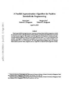
Figure 3: The states ρ1 , ρ2 , ρ3 are a transcript of the referee’s conversation with the yes-prover. It follows easily from the unitary equivalence of purifications that a triple (ρ1 , ρ2 , ρ3 ) is a valid transcript if and only ∗ ) for i = 1, 2, 3 where V = I. if it obeys the recursive relation TrMi (ρi ) = TrAi (Vi−1 ρi−1 Vi−1 0 What can be said of the sets Y(V ), P(V )? Let us begin by considering the set Y(V ). As suggested by Figure 3, each element of Y(V ) can be viewed as the final entry ρa in a transcript (ρ1 , . . . , ρa ) of the verifier’s conversation with the yes-prover. Moreover, it is straightforward to use the unitary equivalence of purifications to characterize those a-tuples of density matrices which constitute valid transcripts. This characterization was first noted by Kitaev [Kit02]. Proposition 10 (Kitaev’s consistency conditions [Kit02]). Let V = (|ψi, V1 , . . . , Va+b−1 , Π) be a verifier and let Y(V ) be the set of admissible states for the yes-prover. A given state ρ is an element of Y(V ) if and only if there exist density matrices ρ1 , . . . , ρa ∈ MMV with ρa = ρ and ∗ TrM (ρi ) = TrM (Vi−1 ρi−1 Vi−1 )

for i = 1, . . . , a

where we have written V0 = I and ρ0 = |ψihψ| for convenience. With these observations in mind we consider completely positive and trace-preserving linear maps Φ0 , . . . , Φa−1 : MMV → MV defined by Φ0 : X 7→ Tr(X) TrM (|ψihψ|) Φi : X 7→ TrM (Vi XVi∗ )

for i = 1, . . . , a − 1

These maps specify the feasible region A(V ) of an SDP of the form (1) from Section 1. Moreover, it follows from Kitaev’s consistency conditions (Proposition 10) that (ρ0 , . . . , ρa ) ∈ A(V ) if and only if ρa ∈ Y(V ). Thus, the min-max problem (9) for λ(V ) can equivalently be written λ(V ) =

max hρa , P i .

min

(ρ0 ,...,ρa )∈A(V ) P ∈P(V )

(10)

We have not yet shown that the set P(V ) of measurement operators for the no-prover is compact and convex. But if we assume for the moment that it is then we may already apply Theorem 1 so as to obtain a parallel oracle-algorithm for approximating λ(V ) on input Φ0 , . . . , Φa−1 given an oracle for optimization over P(V ).

20

5.3

Implementation of the oracle for best responses of the no-prover

In order to complete the description of our parallel algorithm for double quantum interactive proofs it remains only to describe the implementation of the oracle for optimization for P(V ) (Problem 1). In this section we establish the following. Proposition 11. Let V = (|ψi, V1 , . . . , Va+b−1 , Π) be a verifier and let P(V ) be the set of admissible measurement operators for the no-prover. There is a parallel algorithm for optimization over P(V ) (Problem 1) with run time bounded by a polynomial in b, 1/δ, and log(dim(MV)). It follows that the algorithm of Figure 1 yields an unconditionally efficient parallel algorithm for approximating λ(V ) given an explicit matrix representation of the verifier V . As mentioned earlier, this instance of optimization over P(V ) (Problem 1) will be rephrased as an SDP of the form (1) (plus some post-processing) so that the algorithm of Section 4 can be reused in the implementation of our oracle. To this end choose any state ρ ∈ MMV and suppose that a (possibly cheating) yes-prover was somehow able to make it so that the registers (M, V) after the interaction with the yes-prover are in state ρ. Let W be a register large enough to admit a purification of ρ and let |ϕi ∈ WMV be any such purification. If the no-prover acts according to (B1 , . . . , Bb ) then the probability of rejection (as per Eq. (8)) is Pr[reject | ρ, (B1 , . . . , Bb )] = kΠBb Va+b−1 Bb−1 · · · B1 Va |ϕik2 . Notice that this quantity also represents the probability of rejection in a different, single-prover interactive proof with a verifier V 0 whose initial state is Va |ϕi. (Formally, the verifier V 0 exchanges b rounds of messages with one of the provers and zero messages with the other.) The unitaries B1 , . . . , Bb could specify actions for either the yes-prover or the no-prover—a choice that depends only upon how we label the components of the verifier V 0 . Since our goal is to reduce optimization over P(V ) (which is a maximization problem) to an SDP of the form (1) (which is a minimization problem), it befits us to view B1 , . . . , Bb as actions for the yes-prover in the interactive proof with verifier V 0 . Let us write 0 , Π0 ) V 0 = (Va |ϕi, V10 , . . . , Vb−1

0 , Π0 ∈ M where V10 , . . . , Vb−1 MVW are given by

Vi0 = Va+i ⊗ IW 0

Π = (I − Π) ⊗ IW .

for i = 1, . . . , b − 1

The private memory register V0 of the new verifier V 0 is identified with the registers (V, W) and communication register M0 of the new verifier is identified with M. Each choice of unitaries (B1 , . . . , Bb ) induces both a measurement operator P ∈ P(V ) and a state ξ ∈ Y(V 0 ) with

 hρ, P i = kΠBb Va+b−1 Bb−1 · · · B1 Va |ϕik2 = 1 − ξ, Π0 and therefore max hρ, P i = 1 − λ(V 0 ) = 1 − min

P ∈P(V )

ξ∈Y(V

0)

 ξ, Π0 .

Moreover, P ∈ P(V ) achieves the maximum on the left side if and only if the unitaries (B1 , . . . , Bb ) that induce P also induce a state ξ ∈ Y(V 0 ) that achieves the minimum on the right side. Incidentally, by identifying elements of P(V ) with elements of A(V 0 ) we have established that the set P(V ) is compact and convex as required by Theorem 1. We are now ready to prove Proposition 11. 21

Proof of Proposition 11. Consider the following algorithm for optimization over P(V ): 1. Use the algorithm of Figure 1 to find ξ ∈ Y(V 0 ) minimizing hξ, Π0 i. 2. Find the unitaries (B1 , . . . , Bb ) that induce ξ. These unitaries also induce a measurement operator P ∈ P(V ) maximizing hρ, P i. Compute P using (B1 , . . . , Bb ) via standard matrix multiplication. We already saw how the algorithm of Figure 1 can be used to accomplish step 1 given an oracle for optimization over P(V 0 ). In this case P(V 0 ) = {Π0 } is a singleton set and thus the oracle for optimization over P(V 0 ) admits a trivial implementation by returning the only element. It remains only to fill in the details for step 2. Recall that the algorithm of Figure 1 finds a near-optimal transcript (ξ0 , . . . , ξb ) ∈ A(V 0 ), meaning that TrM (ξ1 ) = TrM (Va |ϕihϕ|Va∗ )

TrM (ξi+1 ) = TrM (Vi0 ξi Vi0∗ )

for each i = 1, . . . , b − 1.

(Here ξ0 is an arbitrary density matrix that is not used in our construction. The presence of this matrix is an artifact of the identification of Y(V 0 ) with A(V 0 ).) The following algorithm finds the unitaries (B1 , . . . , Bb ): 1. Let Z be a space large enough to admit purifications of ξ1 , . . . , ξb . Write |α0 i = |ϕi|0Z i and V00 = Va . 2. For each i = 1, . . . , b: (a) Compute a purification |αi i ∈ ZMVW of ξi . 0 |α (b) Compute a unitary Bi ∈ MZM that maps Vi−1 i−1 i to |αi i. 3. Return the desired unitaries (B1 , . . . , Bb ). Correctness of this construction is straightforward (though notationally cumbersome). Let us argue that each individual step consists only of matrix operations that are known to admit an efficient parallel implementation, from which it follows that the entire construction is efficient. Step 2a requires that we compute a purification |αi of a given mixed state ξ. This can be achieved by computing a spectral decomposition X ξ= µi |φi ihφi | i

of ξ; the purification |αi is then given by |αi =

X√ i

µi |φi i|φi i.

Given two pure states |αi, |α0 i ∈ ZMVW with

TrZM (|αihα|) = TrZM (|α0 ihα0 |),

step 2b requires that we compute a unitary B ∈ MZM that maps |αi to |α0 i. This can be achieved by computing Schmidt decompositions X X |αi = si |φi i|ψi i |α0 i = s0i |φ0i i|ψi i i

i

with respect to the partition ZM ⊗ VW. (Schmidt decompositions on vectors are equivalent to singular value decompositions on matrices and hence can be implemented inP parallel.) The desired unitary is then given by straightforward matrix multiplication and summation: B = i |φ0i ihφi |. 22

5.4

Containment of DQIP inside PSPACE

The argument by which a parallel algorithm for double quantum interactive proofs leads to a proof of DQIP ⊆ PSPACE is by now a familiar one. (See Section 3 of Ref. [JJUW11] for a good exposition of this type of argument.) Proof of Theorem 2. For each decision problem L ∈ DQIP we must prove that there is a polynomial space algorithm for L. To this end consider a “scaled up” version of NC known as NC(poly), which consists of all functions computable by polynomial-space uniform Boolean circuits of polynomial depth. It has long since been known that NC(poly) algorithms can be simulated in polynomial space [Bor77], so in order to prove L ∈ PSPACE it suffices to give an NC(poly) algorithm for L. Let V be a verifier with completeness c, soundness s, and polynomial-bounded p with c − s ≥ 1/p witnessing the membership of L in DQIP. Let x be any input string and consider the following algorithm for deciding whether x is a yes-instance or a no-instance of L: 1. Compute an explicit matrix representation of the verifier V = (|ψi, V1 , . . . , Va+b−1 , Π) on input x. As argued earlier, this representation specifies sets A(V ), P(V ) for a min-max problem of the form (2). 2. Compute a δ-approximation of λ(V ) for the choice δ = (c − s)/3 so as to determine which of the two provers has a winning strategy. Accept or reject accordingly. The dimension dim(MV) = 2m+v of the matrix representation of a verifier on input x might grow exponentially in the bit length of x. Nevertheless, as argued in Ref. [JJUW11] for ordinary quantum interactive proofs, it is not difficult to see that step 1 admits a straightforward implementation in NC(poly) via standard matrix multiplication. Earlier in this section we argued that the parallel oracle-algorithm of Theorem 1 can be used to compute the desired approximation of λ(V ). We also presented a parallel implementation of the oracle for optimization over P(V ) required by Theorem 1. To see that this parallel algorithm is efficient it suffices to observe that the number of rounds a + b and the inverse of the accuracy parameter 1/δ both scale as a polynomial in |x| and hence also in log(dim(MV)). Thus, the above algorithm computes the composition of a function in NC(poly) with another function in NC. As NC(poly) is closed under such compositions, it follows that the above algorithm admits an NC(poly) implementation and hence also a polynomial-space implementation. It follows that L ∈ PSPACE and hence DQIP ⊆ PSPACE.

6 6.1

Consequences and extensions A direct polynomial-space simulation of QIP

As mentioned in the introduction, a special case of our result is a direct polynomial-space simulation of multi-message quantum interactive proofs, resulting in a first-principles proof of QIP ⊆ PSPACE. Recall that an ordinary, single-prover quantum interactive proof is a double quantum interactive proof in which the verifier exchanges zero messages with the no-prover. We already observed in Section 5.3 that such a verifier induces an SDP of the form (1) in which elements of the feasible region A are identified with strategies for the prover. In this case, Theorem 1 yields an efficient parallel algorithm for finding optimal strategies for the prover in a single-prover quantum interactive proof with no need to specify an oracle.

23

6.2

Finding near-optimal strategies

The algorithm of Figure 1 not only approximates the value λ(A, P) of the min-max problem (2), but it also finds near-optimal points (ρ1 , . . . , ρk ) ∈ A and P ∈ P. By contrast, in Section 5 we were primarily concerned with the problem of approximating only the value λ(V ) of the min-max problem (10). This quantity is the verifier’s probability of rejection when both provers act optimally; approximating it suffices to prove DQIP ⊆ PSPACE. However, our result readily extends to the related search problem of finding near-optimal strategies for the provers. Indeed, step 4 of the algorithm of Figure 1 returns a transcript (ρ0 , . . . , ρa ) ∈ A(V ) and a measurement operator P ∈ P(V ), both of which are δ-optimal for λ(V ). The unitaries (A1 , . . . , Aa ) for the yes-prover can be recovered from the transcript (ρ0 , . . . , ρa ) via the method described in Section 5.3 with no additional complication. It is only slightly more difficult to recover the no-prover’s unitaries (B1 , . . . , Bb ) from P . Our definition of Problem 1 (Optimization over P) specifies only that a solution produce a near-optimal measurement operator P ∈ P for a given state ρ. But the algorithm for Problem 1 described in Section 5.3 for optimization over P(V ) produces its output P by first constructing the associated unitaries (B, . . . , Bb ). It is a simple matter to modify our definition of Problem 1 so as to also return those unitaries in addition to P . The near-optimal measurement operator P returned in step 4 of the algorithm of Figure 1 is given by T 1 X (t) P = P , T t=1

which indicates a strategy for the no-prover that selects t ∈ {1, . . . , T } uniformly at random and then acts (t) (t) according to (B1 , . . . , Bb ). It is a simple matter to construct unitaries (B1 , . . . , Bb ) that implement this probabilistic strategy by sampling the integer t during the first round, recording that integer in the no-prover’s private memory (which must be enlarged slightly to make room for it), and controlling the operation in subsequent turns on the contents of that integer. All of the matrix operations required to construct (B1 , . . . , Bb ) (t) (t) from each (B1 , . . . , Bb ) in this way can be implemented efficiently in parallel.

6.3

Robustness with respect to error

In Section 1.3.1 we noted that it is not immediately obvious that the classes DIP and DQIP are robust with respect to completeness and soundness parameters c, s. Because of this we defined the classes to be inclusive as possible, allowing any verifier for which c − s ≥ 1/p for some polynomial-bounded function p(|x|). Nevertheless, it follows from the collapse of these classes to PSPACE that they are indeed robust with respect to completeness and soundness. In particular, classical interactive proofs for PSPACE [LFKN92, Sha92] imply that if a decision problem L admits a double (quantum) interactive proof with c − s ≥ 1/p then L also admits a double (quantum) interactive proof with c = 1 and s ≤ 2−q for any desired polynomialbounded function q(|x|). However, the method by which the original verifier is transformed into the low-error verifier is very circuitous: the original verifier must be simulated in polynomial space according to Theorem 2 and then that polynomial-space computation must be converted back into an interactive proof with perfect completeness and exponentially small soundness according to proofs of IP = PSPACE. It would be nice to know whether a more straightforward transformation such as parallel repetition followed by a majority vote could be used to reduce error for double quantum interactive proofs and other bounded-turn interactive proofs with competing provers. 24

6.4

Arbitrary payoff observables

In the study of interactive proofs attention is generally restricted to the accept-reject model wherein the verifier’s measurement {Π, I − Π} indicates only acceptance or rejection without specifying a payout to the provers. From a game-theoretic perspective, one might wish to consider a more general verifier whose final measurement {Πa }a∈Σ could have outcomes belonging to some arbitrary finite set Σ. In this case, the verifier awards payouts to the provers according to a payout function v : Σ → R where v(a) denotes the payout to the yes-prover in the event of outcome a. (Since the game is zero-sum, the no-prover’s payout must be −v(a).) Jain and Watrous describe a simple transformation by which their algorithm for one-turn quantum games can be used to approximate the expected payout in this more general setting [JW09]. Their transformation extends without complication to double quantum interactive proofs. In our case, the expected payout to the yes-prover when she and the no-prover play according to (A1 , . . . , Aa ) and (B1 , . . . , Bb ), respectively, is given by X v(a)hφ|Πa |φi = hφ|ΠΣ |φi a∈Σ

where |φi = Bb Va+b−1 Bb−1 · · · B1 Va Aa Va−1 Aa−1 · · · A2 V1 A1 |ψi P is the final state of the system and the Hermitian operator ΠΣ = a∈Σ v(a)Πa denotes the payout observable induced by the verifier. The expected payout of this interaction can be computed simply by translating and rescaling ΠΣ so as to obtain a measurement operator 0  Π  I and then running our algorithm for double quantum interactive proofs with verifier V = (|ψi, V1 , . . . , Va+b−1 , Π). The expected payout of the original protocol is then obtained by inverting the scaling and translation operations by which Π was obtained from ΠΣ . As noted by Jain and Watrous, this transformation has the effect of inflating the additive approximation error δ by a factor of kΠΣ k, which is the maximum absolute value of any given payout.

Acknowledgements An extended abstract of this paper has appeared as Ref. [GW12]. The authors are grateful to Tsuyoshi Ito, Rahul Jain, Zhengfeng Ji, Yaoyun Shi, Sarvagya Upadhyay, John Watrous, and an anonymous reviewer for helpful comments and discussions. Particularly, the alternative formulation of the strategies by density operators and measurements is inspired during the discussion with John Watrous. XW also wants to thank the hospitality and invaluable guidance of John Watrous when he was visiting the Institute for Quantum Computing, University of Waterloo. The research was partially conducted during this visit and was supported by the Canadian Institute for Advanced Research (CIFAR). XW’s research is also supported by NSF grant 1017335. GG’s research is supported by the Government of Canada through Industry Canada, the Province of Ontario through the Ministry of Research and Innovation, NSERC, DTO-ARO, CIFAR, and QuantumWorks.

References [AHK05] Sanjeev Arora, Elad Hazan, and Satyen Kale. The multiplicative weights update method: a meta algorithm and applications. Submitted, 2005. 7 25

[Bor77]

Allan Borodin. On relating time and space to size and depth. SIAM Journal on Computing, 6(4):733–744, 1977. 23

[Fan53]

K. Fan. Minimax theorems. Proceedings of the National Academy of Sciences, 39:42–47, 1953. 2

[FIKU08] Lance Fortnow, Russell Impagliazzo, Valentine Kabanets, and Christopher Umans. On the complexity of succinct zero-sum games. Computational Complexity, 17(3):353–376, 2008. 6 [FK97]

Uriel Feige and Joe Kilian. Making games short. In Proceedings of the 29th ACM Symposium on Theory of Computing (STOC 1997), pages 506–516, 1997. 5, 6

[FKS95]

Joan Feigenbaum, Daphne Koller, and Peter Shor. A game-theoretic classification of interactive complexity classes. In Proceedings of the 10th Conference on Structure in Complexity Theory, pages 227–237, 1995. 5

[FvdG99] Christopher Fuchs and Jeroen van de Graaf. Cryptographic distinguishability measures for quantum mechanical states. IEEE Transactions on Information Theory, 45(4):1216–1227, 1999. arXiv:quant-ph/9712042v2. 9, 11 [GS89]

Shafi Goldwasser and Michael Sipser. Private coins versus public coins in interactive proof systems. In Silvio Micali, editor, Randomness and Computation, volume 5 of Advances in Computing Research, pages 73–90. JAI Press, 1989. 7

[GW05]

Gus Gutoski and John Watrous. Quantum interactive proofs with competing provers. In Proceedings of the 22nd Symposium on Theoretical Aspects of Computer Science (STACS’05), volume 3404 of Lecture Notes in Computer Science, pages 605–616. Springer, 2005. arXiv:cs/0412102v1 [cs.CC]. 6

[GW07]

Gus Gutoski and John Watrous. Toward a general theory of quantum games. In Proceedings of the 39th ACM Symposium on Theory of Computing (STOC 2007), pages 565–574, 2007. arXiv:quant-ph/0611234v2. 6

[GW12]

Gus Gutoski and Xiaodi Wu. Parallel approximation of min-max problems with applications to classical and quantum zero-sum games. In Proceedings of the 27th IEEE Conference on Computational Complexity (CCC 2012), pages 21–31, 2012. arXiv:1011.2787 [quant-ph]. 25

[JJUW11] Rahul Jain, Zhengfeng Ji, Sarvagya Upadhyay, and John Watrous. QIP=PSPACE. Journal of the ACM, 58(6):article 30, 2011. 4, 6, 7, 8, 9, 23 [JUW09]

Rahul Jain, Sarvagya Upadhyay, and John Watrous. Two-message quantum interactive proofs are in PSPACE. In Proceedings of the 50th IEEE Symposium on Foundations of Computer Science (FOCS 2009), pages 534–543, 2009. arXiv:0905.1300v1 [quant-ph]. 7, 10, 11

[JW09]

Rahul Jain and John Watrous. Parallel approximation of non-interactive zero-sum quantum games. In Proceedings of the 24th IEEE Conference on Computational Complexity (CCC 2009), pages 243–253, 2009. arXiv:0808.2775v1 [quant-ph]. 4, 6, 7, 25

[JY11]

Rahul Jain and Penghui Yao. A parallel approximation algorithm for positive semidefinite programming. In Proceedings of the 52nd IEEE Symposium on Foundations of Computer Science (FOCS 2011), pages 463–471, 2011. arXiv:1104.2502v1 [cs.CC]. 3, 4, 8 26

[JY12]

Rahul Jain and Penghui Yao. A parallel approximation algorithm for mixed packing and covering semidefinite programs. arXiv:1201.6090v1 [cs.DS], 2012. 3, 4, 8

[Kal07]

Satyen Kale. Efficient algorithms using the multiplicative weights update method. PhD thesis, Princeton University, 2007. 7, 8, 9, 14

[Kit02]

Alexei Kitaev. Quantum coin-flipping. Presentation at the 6th Workshop on Quantum Information Processing (QIP 2003), 2002. 8, 20

[KM92]

Daphne Koller and Nimrod Megiddo. The complexity of two-person zero-sum games in extensive form. Games and Economic Behavior, 4:528–552, 1992. 5

[KMvS94] Daphne Koller, Nimrod Megiddo, and Bernhard von Stengel. Fast algorithms for finding randomized strategies in game trees. In Proceedings of the 26th ACM Symposium on Theory of Computing (STOC 1994), pages 750–759, 1994. 5 [KW00]

Alexei Kitaev and John Watrous. Parallelization, amplification, and exponential time simulation of quantum interactive proof system. In Proceedings of the 32nd ACM Symposium on Theory of Computing, pages 608–617, 2000. 7

[LFKN92] Carsten Lund, Lance Fortnow, Howard Karloff, and Noam Nisan. Algebraic methods for interactive proof systems. Journal of the ACM, 39(4):859–868, 1992. 6, 24 [LN93]

Michael Luby and Noam Nisan. A parallel approximation algorithm for positive linear programming. In Proceedings of the 25th ACM Symposium on Theory of Computing (STOC 1993), pages 448–457, 1993. 4, 8

[Meg92]

Nimrod Megiddo. A note on approximate linear programming. Information Processing Letters, 42(1):53, 1992. 3

[MW05]

Chris Marriott and John Watrous. Quantum Arthur-Merlin games. Computational Complexity, 14(2):122–152, 2005. arXiv:cs/0506068v1 [cs.CC]. 7

[NC00]

Michael Nielsen and Issac Chuang. Quantum Computation and Quantum Information. Cambridge University Press, 2000. 9, 11

[Pap94]

Christos Papadimitriou. Computational Complexity. Addison-Wesley, 1994. 2

[PT12]

Richard Peng and Kanat Tangwongsan. Faster and simpler width-independent parallel algorithms for positive semidefinite programming. In Proceedings of the 24th ACM symposium on Parallelism in algorithms and architectures (SPAA 2012), pages 101–108, 2012. arXiv:1201.5135 [cs.DS]. 3, 4, 8

[RW05]

Bill Rosgen and John Watrous. On the hardness of distinguishing mixed-state quantum computations. In Proceedings of the 20th Conference on Computational Complexity, pages 344–354, 2005. arXiv:cs/0407056v1 [cs.CC]. 9

[Ser91]

Maria Serna. Approximating linear programming is log-space complete for P. Information Processing Letters, 37(4):233–236, 1991. 3

[Sha92]

Adi Shamir. IP = PSPACE. Journal of the ACM, 39(4):869–877, 1992. 6, 24 27

[TX98]

Luca Trevisan and Fatos Xhafa. The parallel complexity of positive linear programming. Parallel Processing Letters, 8(4):527–533, 1998. 4

[vN28]

John von Neumann. Zur theorie der gesellschaftspiele. Mathematische Annalen, 100(1):295– 320, 1928. In German. 2

[vzG93]

Joachim von zur Gathen. Parallel linear algebra. In John H. Reif, editor, Synthesis of Parallel Algorithms, chapter 13. Morgan Kaufmann Publishers, Inc., 1993. 7

[Wat11]

John Watrous. Lecture notes: Theory of quantum information. Available on the author’s web page, 2011. 9

[WK06]

Manfred Warmuth and Dima Kuzmin. Online variance minimization. In Proceedings of the 19th Conference on Learning Theory, volume 4505 of Lecture Notes in Computer Science, pages 514–528, 2006. 7

[Wu10]

Xiaodi Wu. Equilibrium value method for the proof of QIP=PSPACE. arXiv:1004.0264v2 [quant-ph], 2010. 7, 9

[You01]

Neal Young. Sequential and parallel algorithms for mixed packing and covering. In Proceedings of the 42nd IEEE Symposium on Foundations of Computer Science (FOCS 2001), pages 538– 546, 2001. 4, 8

28