1 (left) shows the streamlines for Reynolds 400 for the cav-101 mesh. We may .... 5.2 Flow through a Los Angeles class submarine. This problem consists on a ...
Parallel Edge-Based Inexact Newton Solution of Steady Incompressible 3D Navier-Stokes Equations Renato N. Elias, Marcos A. D. Martins, Alvaro L. G. A. Coutinho Center for Parallel Computations and Department of Civil Engineering Federal University of Rio de Janeiro, P. O. Box 68516, RJ 21945-970 – Rio de Janeiro, Brazil {renato,marcos,alvaro}@nacad.ufrj.br
Abstract. The parallel edge-based solution of 3D incompressible Navier-Stokes equations is presented. The governing partial differential equations are discretized using the SUPG/PSPG stabilized finite element method [5] on unstructured grids. The resulting fully coupled nonlinear system of equations is solved by the inexact Newton-Krylov method [1]. Matrix-vector products within GMRES are computed edge-by-edge, diminishing flop counts and memory requirements. The non-linear solver parallel implementation is based in message passing interface (MPI). Performance tests on several computers, such as the SGI Altix, the Cray XD1 and a mini-wireless cluster were carried out in representative problems and results have shown that edge-based schemes require less CPU time and memory than element-based solutions.
1 Introduction We consider the simulation of steady incompressible fluid flow governed by NavierStokes equations using the stabilized finite element formulation in [5]. This formulation allows that equal-order-interpolation velocity-pressure elements are employed by introducing two stabilization terms: the Streamline Upwind PetrovGalerkin (SUPG) and the Pressure Stabilizing Petrov Galerkin stabilization (PSPG). When discretized, the incompressible Navier-Stokes equations give rise to a fully coupled velocity-pressure system of nonlinear equations due the presence of convective terms in momentum equation. The inexact Newton method [1] associated with a proper preconditioned iterative Krylov solver, such as GMRES, presents an appropriated framework to solve nonlinear systems, offering a trade-off between accuracy and the amount of computational effort spent per iteration. Inspired by finite volume methods, edge-based data structures have been introduced for explicit finite element computations of compressible flows on unstructured grids composed by triangles and tetrahedra. Soto et al [11] recently introduced an edge-based approach to solve incompressible flows with an uncoupled fractional step formulation. The advantages of edge-based schemes with respect to conventional element-based schemes are a major reduction in indirect addressing (i/a) operations and memory requirements.
When dealing with large scale problems the use of parallel solvers is an essential condition and the use of an algorithm able to run efficiently in shared, distributed or hybrid memory systems has been a motivation for many researchers to turn the solver strategy more independent of the hardware resources. Therefore, the main goal of this work is the development of edge-based data structures for the SUPG/PSPG finite element formulation to solve steady incompressible fluid flows by a parallel inexactNewton method. The remainder of this work is outlined as follows: next section briefly describes the governing equations and finite element formulation. The third section presents some remarks on edge-based data structures for unstructured grids. The subsequent section treats the parallel implementation, results and final comments are summarized in the last sections.
2 Governing Formulation
Equations
and
SUPG/PSPG
Finite
Element
Let Ω ⊂ \nsd be the spatial domain, where nsd is the number of space dimensions. Let Γ denote the boundary of Ω. We consider the following velocity-pressure formulation of the Navier-Stokes equations governing steady incompressible flows: ρ(u ⋅ ∇u − f)− ∇ ⋅ σ = 0, on Ω
(1)
∇ ⋅ u = 0, on Ω
(2)
where ρ and u are the density and velocity, σ is the stress tensor. The essential and natural boundary conditions associated with equations (1) and (2) can be imposed at different portions of the boundary Γ and represented by, u = g
on Γg
n⋅σ = h
;
on Γh
(3)
where Γg and Γh are complementary subsets of Γ. Let us assume following [5] that we have some suitably defined finite-dimensional trial solution and test function spaces for velocity and pressure, S uh , Vuh , S ph and Vph = S ph . The finite element formulation of equations (1) and (2) using SUPG and
PSPG stabilizations for incompressible fluid flows can be written as follows: find uh ∈ S uh and p h ∈ S ph such that ∀wh ∈ Vuh and ∀q h ∈ Vph :
∫w
h
⋅ ρ(u h ⋅ ∇u h − f )d Ω +
Ω
∫ ε(w ):σ(p h
Ω
h
, u h )d Ω +
∫q
h
∇ ⋅ u hd Ω
Ω
nel
+∑ ∫ τSUPG uh ⋅ ∇wh ⋅ ⎡⎢ ρ( uh ⋅ ∇uh )− ∇ ⋅ σ( ph , uh )− ρf ⎤⎥ d Ω ⎣ ⎦ e =1 Ω
(4)
nel
+∑ ∫
e =1 Ω
1 τ ∇q h ⋅ [ ρ(uh ⋅ ∇uh )− ∇ ⋅ σ(p h , uh )− ρf ]d Ω = ρ PSPG
∫ wh ⋅ h d Γ Γ
In the above equation nel is the number of elements in the mesh. The first four integrals on the left hand side represent terms that appear in the Galerkin formulation of the problem (1)-(3), while the remaining integral expressions represent the additional terms which arise in the stabilized finite element formulation. Note that the stabilization terms are evaluated as the sum of element-wise integral expressions. The first summation corresponds to the SUPG (Streamline Upwind Petrov/Galerkin) term and the second to the PSPG (Pressure Stabilization Petrov/Galerkin) term. The spatial discretization of equation (4) leads to a following system of nonlinear equations, F(x) = 0
(5)
where x = (u, p) is a vector of nodal variables comprising both nodal velocities and pressures and F(x) represents a nonlinear vector function. Newton’s method is attractive method to solve the system (5) because it converges rapidly from any sufficiently good initial guess [1]. However, one drawback of Newton’s method is the need to solve a locally linear system at each stage. Computing the exact solution can be expensive if the number of unknowns is large and may not be justified when xk is far from a solution. Thus, one might prefer to compute approximated linear solutions, leading to the following algorithm, ALGORITHM IN for k = 0 step 1 until convergence do Find some ηk ∈ [0,1) AND sk that satisfy
||F(xk)+J(xk) sk|| ≤ ηk ||F(xk)||
(6)
set xk+1 = xk + sk
for some adaptively chosen ηk ∈ [0,1), where || • || is a norm of choice. The Jacobian, J(xk), is numerically approximated using Taylor’s expansions as described by Tezduyar [6]. This formulation naturally allows the use of an iterative solver like GMRES or BiCGSTAB: one first chooses ηk and then applies the iterative solver to (6) until a sk is determined for which the residual norm is satisfied. In this context ηk is called as a forcing term and can be specified in several different forms as described in [2].
3 Edge-Based data structures Edge-based data structures operate directly in the nodal graph of the underlying unstructured grid. It was shown in [3] that for unstructured grids edge-based data structures have more advantages than element-by-element (EBE) and compressed storage row (CSR) schemes. In the edge-based strategies, global coefficients are computed and stored in single DO-LOOPS making the evaluation of the left and hand
sides faster and less memory demanding. We may derive an edge-based finite element framework by noticing that the element matrices can be disassembled into their contributions as shown in [7, 8]. For the set of all elements sharing a given edge, we may add their contributions, arriving to the edge matrix, which for the problem at hand is a non-symmetric 16 × 16 matrix. In Table 1 we compare the storage requirements to hold the coefficients of the element and edge matrices as well as the flop count and indirect addressing (i/a) operations to compute sparse matrix-vector products in the Krylov iterative driver element-by-element or edge-by-edge, that is, ne
Jp =
Jl pl , ∑ l =1
(7)
where ne is the total number of local structures (edges or elements) in the mesh and pl is the restriction of p to the edge or element degrees-of-freedom. Table 1. Memory to hold the matrix coefficients and computational costs for element and edgebased matrix-vector products for tetrahedral finite element meshes. Memory
Flop
i/a
Elements
1056 nnodes
2112 nnodes
1408 nnodes
Edges
224 nnodes
448 nnodes
448 nnodes
All data in this table is referred to nnodes, the number of nodes in the finite element mesh. According to [9], the following estimates are valid for unstructured 3D grids, nel ≈ 5.5×nnodes, nedges ≈ 7×nnodes, where nedges is the number of edges in the mesh. We may observe that data in Table 1 favors the edge-based scheme.
4 Parallel Implementation The parallel inexact nonlinear solver presented in the previous section was implemented based in the message passing parallelism model (MPI). The original unstructured grid was partitioned into non-overlapped sub-domains by the use of the METIS_PartMeshDual routine provided by Metis package [4]. Afterwards, the partitioned data was reordered to avoid indirect memory addressing and IF clauses inside hot loops and MPI communications. Therefore, the equation numbers shared by the partitions were relocated to the last entries of the corresponding arrays. Most of the computational effort spent during the iterative solution of linear systems is due to evaluations of matrix-vector products or matvec for short. In our tests matvec operations achieved 92% of the total computational costs. In element-byelement (EBE) and edge-by-edge (EDE) data structures this task is message passing parallelizable by performing matvec operations at each partition level, then assembling the contribution of the interface equations calling MPI_AllReduce routine over the last array entries. Finally, it is important to note that edge (and element) matrix coefficients are computed in single DO-LOOPS also in each partition.
5 Results This section presents two benchmark problems to analyze the parallel solver performance. The numerical procedure considers a fully coupled u-p version of the stabilized formulation using linear tetrahedron elements. The parallel solver is composed by an outer inexact-Newton loop and an inner GMRES(25) with nodal block diagonal preconditioned linear solver. The computations were made on two SGI Altix 3700 systems (32/64 Intel Itanium2 CPUs with 1.3/1.5 GHz and 128/256 Gb of NUMA flex memory), and a Cray XD1 system (32 AMD Opteron CPUs with 1.8 GHz). Some portability and mobile parallelism tests were performed on a mini-cluster fast-ethernet/wireless composed by 4 laptop nodes with Intel Centrino processors and Microsoft Windows platform. The same code was compiled for three different systems (Intel Fortran 8.1 on SGI Linux systems, Portland Group Fortran on Cray Linux and Compaq Visual Fortran on minicluster Intel/Windows). No CPU optimizations besides those provided by standard compiler flags (-O3) were made. 5.1 Three dimensional leaky lid-driven cavity flow In this well known problem the fluid confined in a cubic cavity is driven by the motion of a leaky lid. Boundary conditions consist in a unit velocity specified along the entire top surface and zero velocity on the other surfaces. Table 2 shows the problem dimensions employed for all parallel performance tests, where in the label cav-nn, nn means the number of line divisions through the x, y, and z dimensions for mesh construction purposes. Fig. 1 (left) shows the streamlines for Reynolds 400 for the cav-101 mesh. We may note the main vortex formation and the singularities at the cavity corners, typical for this problem. Fig. 1 (right) show the computed vertical and horizontal velocities at the centerline, together with the recent numerical results of Lo et al [13] and Shu et al [14]. We may observe that all results are in good agreement. Table 2. Problem dimensions
cav-31 cav-51 cav-71 cav-101
Elements 148,955 663,255 1,789,555 5,151,505
Edges 187,488 819,468 2,193,048 6,273,918
Nodes 32,768 140,608 373,248 1,061,208
Equations 117,367 525,556 1,421,776 4,101,106
1.00 Lo et al. [13] 0.80
Shu et al. [14] Present
0.60
Lo et al. [13] Shu et al. [14] Present
Vertical velocity (Vz )
0.40 0.20 0.00 -0.20 -0.40 -0.60 -0.80
-1.00 -1.00 -0.80 -0.60 -0.40 -0.20
0.00
0.20
0.40
0.60
0.80
1.00
Horizontal velocity (V x )
Fig. 1. (left) Streamlines in a leaky lid-driven cubic cavity (right) Characteristic results for vertical and horizontal velocity at the centerline.
In Fig. 2 (left) is shown the scaled speedup on the SGI Altix computed according to Gustafson’s law [10] and defined by Ss= n+(1-n) s, where n is the number of processors and s corresponds to the normalized time spent in the serial portion of the program. The scalability reached on SGI Altix for the models listed in Table 2 is shown in Fig. 2 (right). Note that when increasing the problem size the serial fraction s tends to shrink as more processors are employed. In our tests with SGI Altix 3700 we have employed up to 32 Intel’s Itanium-2 processors and according to [10] the scaled speedup should be a linear function with moderate slope 1-n such as the line we have measured and shown in Fig. 2 (right). 35
32 30.43x
28
30
Line
30.19x 28.45x
25
22.20x
M easured
20 16
Speedup
Scaled speedup
24
30.43x
15.69x
12 8
5
4.16x 2.13x 1.00x
0 0
4
8
15 10
8.05x
4
20
12
16
20
24
28
32
0 0.05
0.10
0.15
Number of CPUs
0.20
0.25
0.30
0.35
Serial Fraction
Fig. 2. (left) Scaled speedup on SGI Altix for EDE data structure and cav101 model. (right) Scalability for the models considered.
The scaled efficiency on SGI Altix for EDE data structure is presented in Fig. 3 (left). Good results may be observed for the cavity models, especially for those with larger number of degrees of freedom. In some cases efficiencies greater than 100% may be attributed to cache effects. The time spent when solving the cav-71 problem with EBE and EDE data structures is plotted in Fig. 3 (right). We may observe that the EDE solutions were faster than the EBE in all cases. Nevertheless, the CPU time ratios
between EBE and EDE solutions are around 2.5 up to 16 processors. For 32 processors this ratio decreases. This is an indication that as we refine the meshes, CPU time ratios between EBD and EDE has a tendency to remain around this value. Cav71
Cav101
60 40
Wall time (seconds)
69
80
89 94 95
95 99 98 85
Scaled Efficiency
4000 Element Simple edge
3500
91
94
101 104 104
106 107 99 90
100
Cav51
99 102 101
Cav31 120
3000 2500 2000 1500 1000 500
20
0 1
0 2
4
8
16
2
32
4
8
16
32
Number of CPUs
Number of CPUs
Fig. 3. (left) Scaled efficiency for EDE data structure on SGI Altix. (right) Wall time comparisons for EBE and EDE data structures for cav-71 mesh.
The inexact nonlinear solver behavior is sketched in Fig. 4 through the decrease of relative residual (left), GMRES tolerance, and nonlinear iteration time (right). Note that at the beginning of the solution procedure the linear tolerance is large enough to allow very fast nonlinear iterations. When a sudden decay in the relative residual is detected, as may be seen in nonlinear iterations 14 to 24, the inexact nonlinear method identifies that the desired solution is imminent and the linear tolerance is tightened to entrap the final solution. 2500
1.20
0.00
GMRES tolerance Iteration time
-1.00 1.00
-2.00
2000
GMRES Tolerance
log10( ||r||/||r0|| )
-4.00 -5.00 -6.00 -7.00
0.80
1500 0.60
1000 0.40
-8.00 -9.00
500
0.20
-10.00
Iteration time (seconds)
-3.00
Cav 51x51x51
-11.00
0
0.00
0
2
4
6
8 10 12 14 16 18 20 22 24 26 28 30 Nonlinear iteration
0
2
4
6
8
10 12 14 16 18 20 22 24 26 28
Nonlinear tolerance
Fig. 4. (left) Relative nonlinear residual. (right) GMRES tolerance (bars) controlled by inexact nonlinear method and time per nonlinear iteration (lines)
Fig. 5 shows the results of tests performed on a mini-cluster formed by 4 laptops and a wireless/fast-ethernet network (2 Intel Centrino 1.6 GHz/512Mb, 1 Intel Centrino 1.3 GHz /512Mb and 1 Intel Pentium 4 2.4 GHz/512Mb interconnected by a Linksys
Wireless-B Hub, IEEE 802.11b/2.4GHz/11Mbps or Fast-Ethernet 10/100Mbps network). These tests show the versatility and portability that message passing codes can offer, making possible the solution of even large scale problems employing modest machines.
2750.00
WIRELESS FAST-ETHERNET
2314.91
3000.00 2500.00 2000.00 1750.00 1500.00
250.00
154.52
500.00
178.69
750.00
523.02
1000.00
398.66
1250.00
398.66
Time (sec)
2250.00
0.00 1
2
4
Number of Cluster Nodes
Fig. 5. (Left) Minicluster mobile wireless/fast-ethernet, (Right) Performance comparison between wireless and fast-ethernet networks.
Fig. 5 (right) shows that the wireless technology employed (Wireless-B) was not able to deliver the bandwidth required to reach a desirable speedup in this irregular MPI parallel computation. However, with the increasing bandwidth in wireless technology mobile-parallel computations will be a reality in the near future. The low speedups achieved in the minicluster with fast-ethernet network were also due to the small problem size, as occurred in the case shown in Fig. 3 (left) for SGI Altix. 5.2 Flow through a Los Angeles class submarine This problem consists on a simplified three-dimensional simulation of a laminar flow around a Los Angeles class submarine. The detailed solution and discussion of this problem, involving transient and turbulent flow is given in [12]. Fig. 6 (left) shows the mesh over the submarine hull. The volume mesh comprises 504,947 tetrahedral elements, 998,420 edges and 92,564 nodes. The solution for this problem is shown in Fig. 6 (right), where the pressure contour is plotted over the submarine hull and the velocity in two longitudinal cutting planes. For this problem the linear tolerance oscillated from the maximum value of 0.99 to a minimum of 2.7×10⁻² and the computations were carried out until a minimum relative residual of 10-10 was reached after 21 nonlinear iterations. Fig. 7 (left) shows some comparisons between the systems employed in our tests with EDE data structure. We may see only slight differences between the systems. In Fig. 7 (right) we compare the solution time spent to solve the problem with EBE and EDE data structures. Note again that the EDE data structure running in one CPU was faster than EBE employing four CPUs.
Fig. 6. (Left) Surface mesh, (Right) Typical solution - hull surface (pressure contour), cut planes (velocity contour).
9000
1600.00
Cray XD1 (Opteron 1.8 GHz)
7000
SGI ALTIX 3700 (Itanium-2 1.5 GHz)
Time (seconds)
Time (seconds)
1200.00 1000.00 800.00 600.00
Element Simple edge
8000
SGI ALTIX 3700 (Itanium-2 1.3 GHz)
1400.00
6000 5000 4000 3000
400.00
2000
200.00
1000 0
0.00 1
2
4 8 Number of CPUs
16
32
1
2
4
8
16
32
Number of CPUs
Fig. 7. (Left) Message passing performance in SGI Altix and Cray XD1 – edge-based data structure, (Right) Data structure comparisons on SGI Altix (MPI).
6 Conclusions We have tested the performance of a parallel edge-based inexact Newton solver for fully coupled velocity-pressure nonlinear systems of equations arising from the SUPG/PSPG finite element formulation of steady incompressible flow on unstructured grids. We observed that the inexact nonlinear method employed has shown good balance between accuracy and computational effort. The edge data structure decreased the solution time even without employing any data reordering method to exploit the cache. Our tests with benchmark problems have shown good parallel performances, but interface mapping techniques could be used to reduce the amount of data communication. The code is portable across different computer platforms, ranging from a mobile wireless cluster to the SGI Altix 3700 and Cray XD1 systems without any code modifications or CPU guided optimizations.
Acknowledgements The authors would like to thank the financial support of the Petroleum National Agency (ANP, Brazil) and the Center for Parallel Computations (NACAD) and the Laboratory of Computational Methods in Engineering (LAMCE) at the Federal University of Rio de Janeiro. The authors are very grateful for the computational resources provided by Silicon Graphics Inc. (SGI/Brazil) and Cray Inc. We are also indebted to Prof. M. Behr from RWTH Aachen University by the submarine mesh.
References 1. 2. 3. 4. 5. 6. 7. 8. 9. 10. 11. 12. 13. 14.
Dembo, R. S., Eisenstat, S. C. and Steihaug, T., Inexact Newton Methods, SIAM J. Numer. Anal. (1982) 19: 400-408. Eisenstat, S. C. and Walker, H. F., Choosing the Forcing Terms in Inexact Newton Method, SIAM. J. Sci. Comput. (1996) 17–1: 16–32. Ribeiro, F. L. B. and Coutinho, A. L. G. A., Comparison Between Element, Edge and Compressed Storage Schemes for Iterative Solutions in Finite Element Analyses, Int. J. Num. Meth. Engrg. 2005; 63-4:569-588. Karypis G. and Kumar V., Metis 4.0: Unstructured Graph Partitioning and Sparse Matrix Ordering System. Technical report, Department of Computer Science, University of Minnesota, Minneapolis, (1998) http://www.users.cs.umn.edu/~karypis/metis. Tezduyar, T. E., Stabilized Finite Element Formulations for Incompressible Flow Computations, Advances in Applied Mechanics (1991) 28: 1-44. Tezduyar, T. E., Finite Elements in Fluids: Lecture Notes of the Short Course on Finite Elements in Fluids, Computational Mechanics Division – Vol. 99-77, Japan Society of Mechanical Engineers, Tokyo, Japan (1999). Catabriga, L., Coutinho, A. L. G. A., Implicit SUPG solution of Euler equations using edge-based data structures. Comput. Methods in Appl. Mech. and Engrg, 2002, 32(191): 3477-3490. Coutinho, A. L. G. A., Martins, M. A. D., Alves, J. L. D., Landau, L., Moraes, A., Edgebased finite element techniques for non-linear solid mechanics problems. Int. J. Num. Meth. Engrg, 2001, 50(9):2053-2068. Lohner, R., Edges, stars, superedges and chains, Comput. Methods in Appl. Mech. and Engrg 1994, 111(3-4): 255-263. Gustafson, J. L., Montry, G. R. and Benner, R. E., Development of Parallel Methods for a 1024-Processor Hypercube, SIAM J. on Sci. and Stat. Comp., 1988, 9(4):609-638 Soto, O., Löhner, R., Cebral, J. and Camelli, F., A Stabilized Edge-Based Implicit Incompressible Flow Formulation, Comput. Methods Appl. Mech. Engrg. 2004, 193:21392154. http://manila.cats.rwth-aachen.de/developer/cases/la.0808, last visited in May 10, 2005. Lo, D. C., Murugesan, K and Young, D. L., Numerical solution of three-dimensional velocity-vorticity Navier-Stokes equations by finite difference method, Int. J. Numer. Meth. Fluids 2005, 47:1469-1487. Shu, C., Wang, L. and Chew Y T, Numerical computation of three-dimensional incompressible Navier-Stokes equations in primitive variable form by DQ method, Int. J. Numer. Meth. Fluids 2003; 43:345-368.