GS3. 6 1305. 475 2519. 919 4576 1686. 8646 3216 17626 6586 36981 13851. GS5. 10 1784. 380 2515. 535 3522. 750. 5216 1112. 7646 1634 10775. 2315.
Parallel Iterated Methods based on Multistep Runge-Kutta Methods of Radau type K. Burragey
�
H. Suhartantoz
Abstract
This paper investigates iterated Multistep Runge-Kutta methods of Radau type as a class of explicit methods suitable for parallel implementation. Using the idea of van der Houwen and Sommeijer [18], the method is designed in such a way that the right-hand side evaluations can be computed in parallel. We use stepsize control and variable order based on iterated approximation of the solution. A code is developed and its performance is compared with codes based on iterated Runge-Kutta methods of Gauss type and various Dormand and Prince pairs [15]. The accuracy of some of our methods are comparable with the PIRK10 methods of van der Houwen and Sommeijer [18], but require less processors. In addition at very stringent tolerances these new methods are competitive with RK78 pairs in a sequential implementation.
1 Introduction The invention of parallel computers in uences the development of methods for solving initial value problems for systems of ordinary di�erential equations (1.1)
y0 (x) = f(y(x)); y(x0 ) = y0 ; f : Rm ! Rm :
Implicit methods such as Implicit Runge-Kutta (IRK) and Multistep Runge-Kutta (MRK) methods which were not previously of much interest due to the increased number of coupled nonlinear algebraic equations, unless very special structures were imposed on the coe�cient matrix, has now begun to attract more people. However, it was Jackson and N�rsett [23] and van der Houwen and Sommeijer [17] who introduced the iteration of IRK to take advantage of parallelism. Since then various issues have been debated in [21, 25] and [27]. Despite these debates, the results of van der Houwen and Sommeijer [18] showed that codes based on parallel iteration are comparable in accuracy and more e�cient in terms of function evaluation than standard sequential codes such as DOPRI8 which implements high order formulas of Prince and Dormand [15]. Van der Houwen and Sommeijer's work also showed that it is possible to construct high order methods with a minimum number of stage evaluations. Their contribution motivates us to construct higher order methods � draft3.0 y Department of z Department of
Mathematics, University of Queensland, Australia Mathematics, University of Queensland, Australia
1
than their methods with a similar number of internal stages. This is possible since our iterated methods will be based on MRK methods which can be order of 2s+r ? 1, see for example Burrage [3]. The method is characterized by Yi = (1.2)
yn+1 =
r X j =1 r X j =1
s X
aij yn+1?j + h �j yn+1?j + h
j =1 s X j =1
bij f(Yj ); i = 1; : : :; s;
j f(Yj ):
The method is an example of more general class of methods called a multivalue (general linear) methods. The yn+1?i; (i = 1; : : :; r) contain all the information from step to step and are updated at the end of a step by computing f(Y1 ); : : :; f(Ys ), which represent approximations to the derivatives of the solution at s internal points, and taking appropriate linear combination. In section 2 we will review the concepts of MRK methods and, based on the idea of van der Houwen and Sommeijer [18], we will develop iterated methods based on MRK in section 3. The last two sections will be devoted to implementation issues and numerical results.
2 Multistep Runge-Kutta methods The general class of MRK methods have been studied by Butcher [6, 7], Cooper [11], Hairer and Wanner [14], Burrage [3, 2] and Burrage and Moss [1]. In particular, Burrage [3] has studied the order conditions of these methods, and has shown that one can always construct methods of order 2s + r ? 1 based on collocation approximation. By de ning the following relationships: C(p) : B(p) : D(p) :
A�k = ck ? kBck?1 ; k = 0; : : :; p; �T �k = rk ? k T ck?1; k = 0; : : :; p; k T C k?1B = rk T ? T C k ; k = 1; : : :; p;
where A and B are s � r and s � s matrices whose (i; j) elements are aij and bij respectively, � = (0; ?1; : : :; ?r + 1)T ; c = (c1 ; : : :; cs )T ; � = (�1; : : :; �r )T ; = ( 1 ; : : :; s )T ; C = diag(c1 ; : : :; cs) and multiplication of vectors is done componentwise , Burrage [3] has proved
Theorem 1 . A multistep Runge-Kutta method will be of order w if B(w); C(�); D(�) hold where � and � are nonnegative integers such that � � r ? 1; w � � + � + 1; w � 2� + 2. Theorem 2 . A multistep Runge-Kuta method will be of order s + r ? 1 + t if C(s + r ? 1), and
B(s + r ? 1 + t) hold, for t = 1; : : :; s.
Hairer and Wanner [16] view the methods, characterized by Theorem 2, as multistep collocation methods, assuming that one has s real numbers c1 ; : : :; cs and r solution values yn ; : : :; yn+1?r . 2
Thus reverting to the non-autonomous version of (1.1) and de ning the corresponding polynomial u(x) of degree s + r ? 1 by (2.1) (2.2)
u(xj ) = yj ; j = n; : : :; n + 1 ? r
u0(xn + ci h) = f(xn + cih; u(xn + cih)); i = 1; : : :; s;
the numerical solution is then given by (2.3)
yn+1 = u(xn+1):
Now suppose that the derivatives u0(xn + ci h) are known, then (2.1) and (2.2) form a Hermite interpolation problem with insu�cient data since the function values at xn + ci h are not available. In order to overcome this problem the dimensionless coordinate t = (x ? xn )=h; x = xn +th, nodes t1 = ?r + 1; : : :; tr?1 = ?1; tr = 0 are de ned. In addition, the polynomial 'i (t); (i = 1; : : :; r) of degree s + r ? 1 is de ned by �
0 if i 6= j 1 if i = j j = 1; : : :; r '0i (cj ) = 0; j = 1; : : :; s and polynomial i (t) (i = 1; : : :; s) is de ned by 'i (tj ) =
(2.4)
i (tj )
= 0; j = 1; : : :; r � 1 if i = j j = 1; : : :; s: 0 i (cj ) = 0 if i 6= j
(2.5)
Now polynomial u(x) can be written as (2.6)
u(xn + th) =
r X j =1
'j (t)yn+1?j + h
s X j =1
j (t)u0 (xn + cj h):
In (2.6) if we put t = ci , and writing u(xn +ci h) = vi then inserting the collocation condition (2.2) gives (2.7)
vi =
(2.8)
yn+1 =
r X j =1 r X j =1
'j (ci )yn+1?j + h 'j (1)yn+1?j + h
s X
j =1 s X j =1
j (ci )f(xn + cj h; vj );
i = 1; : : :; s
j (1)f(xn + cj h; vj );
which is the MRK formula (1.2) where aij = 'j (ci ); bij = j (ci ); �j = 'j (1); and j = j (1). 3
The highest possible order of the method depends on the way one chooses the nodes ci. Burrage[3], Guillou & Soule [13] and Lie & N�rsett [26] constructed a method of maximal order p = 2s + r ? 1. But these methods are not sti�y stable and are not suitable for sti� problems. Since this paper represents the rst of a series of papers in which we hope to develop a type sensitive code based on MRKs, it will be necessary to have a sti�y stable corrector for the sti� part, and so we will also use this corrector for the nonsti� part. Thus we consider methods of Radau type by choosing cs = 1 and try to determine the remaining nodes ci so that we obtain a method of order p = 2s + r ? 2. The methods are characterized by the tableau form c A : (2.9) B Hairer and Wanner [16] using the idea of Krylov [24] and adapting to quadrature problems have proved that one can obtain a method of order p = 2s + r ? 2 where the nodes are computed by solving nonlinear equations �0i (ci ) = 0; i = 1; : : :; s ? 1, where �i (t) is de ned as (2.10)
�i (t) = C
r Y
(t ? tj )
j =1
s Y
(t ? cj )2 ;
j =1;j 6=i
and where C�is determined by �i (ci ) = 1. The solution to the ensuing nonlinear equation has � s + r ? 1 solutions, however we consider only the solutions c with 0 < c < 1. Appendix i i r?1 A de nes the method parameters for the (r; s) pairs (2; 2), (2; 3), and (3; 3) as well as for what appears to be the three most e�ective methods namely the (4; 2), (5; 3), and (7; 3) methods. Note that when r = 1 we obtain the class of Radau Runge-Kutta methods of order 2s ? 1 that are sti�y accurate, while when s = 1 we obtain the family of BDF methods. We also note that the class of sti�y accurate methods of order 2s + r ? 2 have been implemented by Schneider [28] who shows that this class of methods can be very e�ective at stringent tolerances for sti� problems.
3 Iterated Multistep Runge-Kutta Methods We start with the iterated method based on general MRK methods, not necessarily of Radau type, by using a Kronecker tensor product form and following the notation of van der Houwen and Sommeijer [18]. Thus we write (1.2) as (3.1)
yn+1 = (�T I)y(n) + h( T I)F(Yn );
where
Yn = (A I)y(n) + h(B I)F(Yn ): T )T , F(Yn) = (f(Yn;1 )T ; : : :; f(Yn;s )T )T , y(n) Here Yn represents s stages vectors (Yn;T 1; : : :; Yn;s T T T represents r previous solutions (yn ; : : :; yn+1?r ) and I denotes the identity matrix of order m. Since we are only concerned with solving non-sti� problems, the implicitly de ned equations above 4
can be solved by some form of xed-point iteration without placing too severe a restriction on the stepsize in terms of a Lipschitz constant for f. Thus after L corrections we obtain the method j = 1; : : :; L Yn(j ) = (A I)y(n) + h(B I)F(Yn(j ?1)); (L) T (n) T yn+1 = (� I)y + h( I)F(Yn ): The computational time needed for one iteration of (3.2) is equivalent to the time required to evaluate one right-hand side function on a sequential computer assuming that there are s processors available and the component of F(Yn(j ) ) is done in parallel. We call a method providing F(Yn(0) ) the predictor method and (3.1) the corrector method, and the resulting parallel, iterated MRK method will be called PIMRK. Let F(Yn(0) ) be an approximation to F(Yn) satisfying the condition (3.2)
(3.3)
(0) f(Yn;i ) = f(Yn;i ) + O(hq ); i = 1; : : :; s;
resulting in yn(0)+1 = yn+1 +O(hq+1 ), then the predictor method satisfying (3.3) is called a predictor method of order q. Since we are using corrector methods of Radau type of order p = 2s + r ? 2, we have that �j = asj ; j = bsj and so yn+1 = (eTs I)Y (L) . Thus assuming that we have a predictor of order q ? 1, we can generalize the result of Jackson and N�rsett [23] and Burrage [5] that the (global) order of yn+1 equals p� = min(p; q + L). Note that for F(Y (0) ) = (e I)f(yn ) one has F(Yn(0) ) = F(Yn) + O(h), i.e., q = 1, and then we have
Theorem 3 . Let A; B; �; de ne an r-step, s-stage MRK methods, and denote F(Yni ) by Fni , ( )
( )
then the PIMRK method de ned by
Fn(0) = (e I)f(yn ); (3.4) Yn(j ) = (A I)y(n) + h(B I)Fn(j ?1); j = 1; : : :; L; yn+1 = (eTs I)Yn(L) ; represents an (L + 1)s-stage explicit MRK method of order p� = min(p; L) requiring L parallel stages. Here eT = (1; 1; : : :; 1) and eTs = (0; 0; : : :; 0; 1):
3.1 Predictor methods
Unlike van der Houwen and Sommeijer [18] who used predictor methods by performing the auxiliary vector recursion we instead use predictor methods which are based on past information. Note that Burrage [4] suggested predictor methods based only on past information on node points, hence the stability function is easily obtained. In addition, Jackiewicz and Tracogna [22] studied a class of two-step Runge-Kutta methods which depend on stage values at two consecutive steps. Their methods, which do not belong in the class of MSRKs, are quite e�cient with respect to the number of function evaluations. Our methods are more general than theirs for we are not limited to two past stages values. 5
With this information we actually could predict either Yn(0) or Fn(0). In the former case, we should evaluate F(Yn(0) ) then start the iteration, while in the latter case we immediately start the iteration saving one function evaluation on every step. We have conducted a number of experiments comparing these two approaches. In terms of accuracy they are comparable, except for predictors using the information on both the node and internal points and then the former case is more accurate than the latter. However, the latter approach is more e�cient in terms of the number of function evaluations for predictors using various values of past information. Observing this phenomena, we do not consider predicting Yn(0). The trivial predictor P0 for Fn(0) is de ned as (f(yn )T ; : : :; f(yn )T )T and gives an iterated method of order p� = min(p; L). We denote predictor Pa , where a represents classes of predictor using speci c past information, with a taking the values 1; 2 , 3 and 4. P1 means the predictor uses derivatives on r previous node points, P2 indicates that the predictor uses both derivatives on r previous node points and s stage points in the previous step, P3 means the predictor uses only derivatives on s stage points, and P4 indicates that the predictor uses derivatives on s previous stage points and tn?1. For example, we consider predictor P1 which uses r previous derivatives fn ; : : :; fn+1?r . We will determine the s � r matrix V1 such that Fn(0) = (V1 I)f (n) ;
(3.5)
where f (n) denotes (f(yn )T ; : : :; f(yn+1?r )T )T . By expanding the solution and the derivatives at tn we obtain the order conditions, pcp?1 = pV1 �p?1 ;
(3.6)
where � = (0; ?1; : : :; ?r + 1)T . It is obvious that Fn(0) is of order r ? 1. Note that (3.6) can be simpli ed into cp?1 = V1�p?1 . Since both c and � are available, then V1 can be obtained by solving systems of linear equations to give an s � r matrix. For P2, P3 and P4, similar systems of equations arise with � de ned as � = (?1 + c1 ; : : :; ?1 + cs?1 ; 0; ?1; : : :; ?r + 1)T , � = (?1 + c1 ; : : :; ?1 + cs?1 ; 0)T , and � = (?1 + c1; : : :; ?1 + cs?1; 0; ?1)T , respectively, where in each of the cases, Vi ; i = 2; 3; 4 is an s � (s + r ? 1); s � s; and s � (s + 1) matrix, respectively.
3.2 Stability
We consider now the linear stability of a PIMRK (based on the trivial predictor) with respect to the test equation (3.7) y0 (t) = �y(t): It is obvious that the application of (3.4) yields the recursion (3.8)
Yn(L) = (I + zB + z 2 B 2 + : : : + z L?1 B L?1 )Ay(n) + z L B L e yn ;
where z = �h. Let m(z) = (I + zB + : : : + z L?1 B L?1 )A then (3.9)
yn+1 = eTs m(z)y(n) + eTs z L B L eyn ; 6
Figure 1: Stability region for (2,2), (4,2), and PIRK, after L = 3 and this takes the form of the recurrence relation (3.10) yn+1 ? �1(z)yn ? : : : ? �r (z)yn+1?r = 0; where �1(z) = eTs z L B L e� + eTs m(z)�e; �j (z) = eTs m(z)e�j ; j = 2; : : :; r: where e�T = (1; : : :; 1) 2 Rr and e�j T are the standard basis vectors for Rr . If we choose L = p, where p is the order of the corrector then we obtain a stability polynomial of degree p. The stability regions of PIMRK methods with pair values (r; s) of (2; 2); (4; 2) and the PIRK method of order 4 based on iterating the s stage Gauss method after L = 3 are given in Figure (1). The PIRK method appears to have a slightly larger stability region than the PIMRK methods but there is little di�erence. Now, we consider the e�ects of various non trivial predictors on the stability polynomial. Since we are using s past derivatives values and r node points for estimating Fn(0), we write (3.11) Fn(0) = (Wi I) f(Zn ); i = 1; : : :; 4; where Wi depends on whether we are using P1; P2; P3 or P4, and Zn = (Yn?1;1; : : :; Yn?1;s; yn?1; : : :; yn+1?r )T 2 Rs+r?1 : Note that Yn?1;s is yn since the method is sti�y accurate. Applying (3.7) we obtain F (0) = �Wi Zn . For the case of P1 ; P2; P3 and P4, respectively, Wi is de ned as � � � � � � � � 0s�(s?1) V1 ; V2 ; V3 0s�(r?1) ; V4 0s�(r?2) ; 7
where 0i�j stands for zero matrix of dimension i by j. So after L iterations, we rewrite the corrector as (3.12) Yn(L) = m(z)y(n) + z L B L Wi Zn ; i = 1; : : :; 4: And this can be further rewritten as (3.13) where
Zn+1 = Mi (z)Zn ; i = 1; : : :; 4; �
�
�
m(z) + z L Mi (z) = 00s�(s?1) J (r ?1)�(s?1) and J is a matrix of dimension r ? 1 � r as follows 2 1 0 ��� 6 0 1 ��� J = 664 0 0 ... 0 0 ���
�
B L Wi 0(r?1)�(s+r?1) ; i = 1; : : :; 4; 0 0 0 1
3
0 0 77 7: 05 0
The characteristic polynomial associated with (3.13) is (3.14)
pi (�; z) = det(Ir+s?1 � � ? Mi (z)); i = 1; : : :; 4;
where Ir+s?1 is the identity matrix of order r + s ? 1. We have computed the stability regions for (r; s) = (2; 2) after L = 3 iterations using predictors P0; P1; P2; P3 and P4, see gure (2). Predictors P0 and P1 give the largest stability regions in this case. Note that the two separate lines in rightmost plots represent boundaries from the Schur's criterion and can be ignored.
3.3 The rate of convergence of the inner iterations
Following the de nition of the rate convergence of the inner iterations by Cong & Mitsui [8], the convergence bound of a PMIRK method is de ned in a similar way as for methods proposed in [9, 10, 19]. We use a test equation y0 (x) = �y(t), where � runs through the eigenvalues of the Jacobian matrix @f=@y, then we obtain the iteration error equation (3.15) Yn(j ) ? Yn = zB[Yn(j ?1) ? Yn]; z = �h; j = 1; : : :; L: So the spectral radius �(B) of the matrix B dominates the rate of convergence. We call �(B) the convergence factor of the PIMRK method. Requiring that �(zB) < 1, gives us the convergence condition in the inner iterations 1 1 or h < (3.16) jz j < �(B) �(B)�(@f=@y) : The convergence factors for particulars PIMRK methods are discussed in the next two section.
8
P2
2
2
y
P0
-2.5
P1
-2
-1.5 x
1
-1
-0.5
P3
00
1
0.5
-2.5
-2
-1.5
-1
-0.5
00
0.5
-1
-1
-2
-2
P4
2
2
y 1
-2.5
-2
-1.5
-1
-0.5
00
1
0.5
-2.5
-2
-1.5 x
-1
-0.5
00
-1
-1
-2
-2
Figure 2: (2,2) with P0; P1; P2; P3 and P4
9
0.5
4 Implementation considerations In this section we describe a simple strategy for implementing PIMRK with a variable stepsize in order to control the local truncation error. r ? 1 starting procedures based on IRK of Radau type of order 2s� ? 1 are used to compute y1 ; : : :; yr?1 where s� is determined so that it is at least the order of the main MRK method, i.e., 2s + r ? 2. Hence s� = d 2s+2r?1 e. Our strategy is similar to the one implemented by van der Houwen and Sommeijer [18] which is also implemented in DOPRI8. If the trivial predictor is used then we de ne L = p so that yn+1 is of O(hp+1 ), since in each iteration we have Ys(j ), which is the approximation of yn+1 of O(hj +1), then at the end of iteration we have Ys(p) of O(hp+1 ). As the result we de ne an estimate of local error � from step n to step n + 1 as (4.1)
� = kyn+1 ? Ys(p?1)k;
for some norm k:k. It is obvious that � = O(hp ). As a matter of fact, one could consider Richardson's strategy for estimating local error, but our few experiments indicated that this approach is more expensive than (4.1). In the xed iteration implementation, a step is accepted when � � TOL and rejected otherwise. The new step size is chosen as 1 p gg: ) (4.2) hnew = h � minf6; maxf 31 ; 0:9( TOL � 1 The constants 6 and 3 in the expression are used to prevent an abrupt change in the stepsize and the safety factor 0:9 is added to increase the probability that the next step will be accepted. The PIMRK method also allows us to implement variable order techniques. This can be done by avoiding xing the number of iterations and using two successive approximation to the solution as the estimate of local error, i.e, �(j ) = kYs(j ) ? Ys(j ?1)k: If during iteration the condition �j � TOL is satis ed for some j = j0 then accept Ys(j0 ) as the numerical solution yn+1 . The next step size will be determined as in (4.2) but �j0 and p� = minfp; q+j0g is used instead of � and p. If the tolerance condition is not satis ed after M iterations, the step will be rejected, h is rede ned and the step is restarted. In the implementation we de ne M = 2s + r ? 2. In this way a variable order PIMRK can be implemented.
5 Numerical experiments In this section we present some numerical experiments which are done in Matlab, on a Sun Sparc2 workstation, whose unit roundo� error is 2:22e?16. The coding in Matlab is convenient since one can perform vector and matrix operation very simply hence requiring less e�ort compared with coding in a conventional programming language, such as Fortran. The performance of parallel computation is estimated by observing the number of function evaluations per processor. 10
5.1 Convergence factors
Table (1) is the result of a direct numerical computation on the convergence factor of PIMRK methods de ned on section 4. Our convergence factors are slightly larger than those of PIRK methods (a class of iterated Runge-Kutta methods, see van der Houwen and Sommeijer [18]) and PITRK ( a class of iterated two step Runge-Kutta methods, see Cong and Mitsui [8]). However our numerical experiments indicated that these di�erences do not greatly a�ect the overall performance of the method. One way of reducing the convergence factors of PIMRK methods is by reducing the order of the methods. For example, for r = 3; s = 2 we have a method of order 5, but reducing it to order 4 we will have one free parameter c1. The parameter is computed in such a way that all eigenvalues of a matrix B^ of the resulting method are minimum. In fact by assuming order s + r ? 1 (with cs = 1) there are s ? 1 free parameters c1 ; : : :; cs?1. We performed this approach on methods (r; s) = (3; 2) and (4; 2) which are of order 5 and 6. The convergence factors of these methods after reducing to order 4 and 5 are respectively :257 and :273. They are indeed smaller than those convergence factors of the original methods, see Table (1). We performed numerical experiments by using the original methods (3; 2) and (4; 2) and their companion methods of order one lower with variable stepsize and variable order strategies on several test problems such as problem A1, A2, A3, Fehlberg from DTEST [12], and a constant problem TC y10 = 0:5; y20 = 100, with various values of tolerances. Tables (2,3,4,5,6) show the number of (sequential) function evaluations required using the predictor P3 . In general, the results show that there is no signi cant improvement obtained by the companion methods. Several cases in which the companion methods are more e�cient are in Table 2 for method (3; 2) at log tolerance ?4, Table 3 for method (3; 2) at log tolerance ?4; ?6; ?8 and for method (4; 2) at log tolerance ?8; ?10; ?12, Table (4) for method (3; 2) at log tolerance ?4; ?6; ?12 and for method (4; 2) at log tolerance ?4; ?6, Table (5) for method (3; 2) at log tolerance ?4; ?6 and for method (4; 2) at log tolerance ?4; ?6, and ?8, and Table (6) for method (3; 2) at log tolerance ?4; ?8 and for method (4; 2) at log tolerance ?8. The star � symbol at Table (6) indicate that the integration is aborted due to too many steps required. Note that in table (5) since the original method is higher order than the companion and the problem solved is a constant ODE, its costs is independent on tolerances. Note also that in table (6), we integrate the problem on a longer interval than in table (13), hence the costs on the table di�er signi cantly. The results also indicate that the convergence factors do not a�ect too much on the performance of the method, for example, method (3; 4) of order 9 with convergence factor :188 is less e�cient than method (6; 3) of order 10 with convergence factor :249. The stability of the method is more dominant than the convergence factor.
5.2 Comparison among (
r; s)
We have solved Van der Pol's equation y10 = y1 (1 ? y22 ) ? y2 ; y20 = y1 ; where the interval of integration is [0; 20] and y0 = (0 ; :25)T . Several (r; s) pairs for r-steps s-stages PIMRK are implemented with the trivial predictor. 11
Table (7) is the result of a xed number of iterations per step, while Table (8) is the result of the variable order implementation. Various values of tolerances are used. The character * in the tables indicates that the program is aborted due to too many steps required. For the sequential cost, we see in Table (7) that higher order methods (5; 3) and (7; 3) with order 9 and 11, respectively are suitable for stringent tolerances, but at less stringent tolerance the lower order methods such as (4; 2) are preferred. Meanwhile in parallel costing, the high order methods such as (4; 4) and (6; 4) are preferred for all values of tolerances. We observe from Table (8) that the variable order implementation of PIMRK works as expected, it is more e�cient than the xed number iteration implementation. The results also shows that higher order PIMRK such as (6; 4); (7; 3) and (7; 4) are suitable both for sequential and parallel implementation with fair to stringent tolerances.
5.3 Comparing predictors
We considered the accucary and the e�ciency of the methods. We solved problem A1, A2, A3, and A4 of [20]. For accuracy comparison, xed stepsize h and xed iteration methods are used. In the test we use r-step s-stages PIMRKs with values of (r; s) as (4; 2); (5; 3) and (7; 3). In Tables (9), (10), (11) and (12) we listed values TP, NFS, NFP, and D which, respectively, denote the type of predictor, the number of function evaluations for sequential machines, the number of function evaluations for parallel machines, and the number of similar digits to the exact solution at the end point of integration (absolute accuracy). Comparing experiments at xed stepsize h, we observed that all type of predictors have comparable accuracy, except P2 which is the least accurate amongst the other type predictors. Next we implement variable order methods with stepsize selection strategy described earlier. On the test, we compare the performance of low order method (4; 2), higher order methods (5; 3) and (7; 3), Gauss3, Gauss5 (van der Houwen and Sommeijer [18]) and RK78 (Dormand and Prince [15]). The results for the Fehlberg problem are given in Table (13), the results for the motion of rigid body without external forces, problem B5 [20], are presented in Table (14), and the results to the Orbit problem, problem D2 [20] are presented in Table (15). These tables also show that the low order methods are suitable for fair tolerances while higher order methods are suitable for stringent tolerances. In a sequential environment the (7; 3) methods are as e�ective as the RK78 pair at very stringent tolerances, while for a parallel implementation a number of our methods are comparable with Gauss5 methods. The advantage being that they are require fewer processors than the 5 processors required for the implementation of Gauss5. The results also indicate that P3 is the most robust predictor.
6 Conclusion We have designed parallel iterated methods based on multistep Runge-Kutta of Radau type. The methods are implemented, and both sequential and parallel costs are examined. The sequential cost indicates that the maximum performance are attained by methods (5; 3) and (7; 3). The performance of methods with orders higher than these are less e�cient. In general a method (r2 ; s2) is less e�cient than (r1; s1 ) where s2 > s1 even though they are the same order, this is 12
due to the fact that (r2; s2 ) requires more function evaluation than (r1; s1 ), see for example (4; 2) and (2; 3), (2; 4) and (4; 3), and (3; 4) and (5; 3) which are respectively, of orders 6, 8, and 9. As we expected the higher methods are preferred for stringent tolerances, in particular those with predictor P3 and P4 have sequential performances comparable to RK78. In the Table (13), at tolerance 10?14 for instance, their sequential performances are even better than those of RK78. We have also seen (from Tables (7) and (8), for example) that the variable order implementation is both more e�cient and robust than the corresponding xed order implementation at all levels of tolerance and suggests that the variable order implementation is the method of choice. In this case the (6; 4) and (7; 4) variable order methods (which have maximum order 12 and 13 respectively) appear to be the most suitable candidate both sequentially and in parallel. In the case of parallel cost estimates, we observed that even though s2 > s1 , method (r2; s2 ) is mostly better than (r1; s1 ). Unlike the performance in sequential cost, the higher order methods gain more e�ciency than lower methods, this motivates us to continue our works on real parallel implementation of the methods so that we could nd suitable methods (r; s) for a multiprocessor environment, in which, for example the the computation of the right-hand side is dominant and costly. This will be considered in a later paper.
References [1] Burrage, K. & Moss, P. M., (1980), Simplifying assumptions for the order of partioned multivalue methods, BIT 20, 452{465. [2] Burrage, K. (1985), Order and stability of explicit multivalue methods, Appl. Numer. Math., 1, 363{379. [3] Burrage, K. (1988), Order properties of multivalue methods, IMA J. Numer. Anal. 8, 43{69. [4] Burrage, K. (1993), The Search for the Holy Grail, or: Predictor-Corrector methods for solving ODEIVPs, App. Num. Math. 11, 125{141. [5] Burrage, K. (1995), Parallel and sequential methods for Ordinary Di�erential Equations, Oxford University Press, New York. [6] Butcher, J.C. (1966), On the convergence of numerical solutions to ordinary di�erential equations, Math. Comp., 20, 1{10. [7] Butcher, J. C. (1973), The order of numerical methods for ordinary di�erential equations, Math. Comp., 27, 793{806. [8] Cong, Nguyen huu & Mitsui, Taketomo (1996), A class of explicit parallel two-step RungeKutta methods, in preparation. [9] Cong, Nguyen huu (1994), Parallel iteration of symmetric Runge-Kutta methods for non sti� initial value problems, J. Comput. Appl. Math., 51, 117{125. [10] Cong, Nguyen huu (1995), Explicit parallel two-step Runge-Kutta-Nystrom methods, to appear in Comput. Math. Appl. 13
[11] Cooper, G. J. (1978), The order of convergence of general linear methods for ordinary di�erential equations, SIAM J. Numer. Anal, 15, 643{661. [12] Enright, W.H & Pryce, J.D. (1987), Two Fortran Packages for Assessing Initial Value Methods, ACM Transactions on Mathematical Software, 13, 1{27. [13] Guillou, A. & Soul�e, J.L. (1969), La r�esolution num�erique des probl�emes di��erentiels aux conditions initiales par des m�ethodes de collocation, R.I.R.O., R-3, 17{44. [14] Hairer, E. & Wanner, G. (1974), On the Butcher group and general multivalue methods, Computing, 13, 1{15. [15] Hairer, E. & Wanner, G. (1987), Solving Ordinary Di�erential Equations I: Nonsti� Problems, Springer Series in Comp. Math., Springer-Verlag, Berlin. [16] Hairer, E., N�rsett, S. P., & Wanner, G. (1991), Solving Ordinary Di�erential Equations II: Sti� and Di�erential-Algebraic Problems, Springer Series in Comp. Math., Springer-Verlag, Berlin. [17] Houwen, P. J. van der & Sommeijer, B. P. (1988), Variable step integration of high order Runge-Kutta methods on parallel computers, Rep. NM-R8817, CWI, Amsterdam, The Netherlands. [18] Houwen, P.J. van der & Sommeijer, B.P. (1990), Parallel iteration of high-order Runge-Kutta methods with stepsize control, J. Comput. Appl. Math. 29, 111{127. [19] Houwen, P. J. van der & Cong, Nguyen huu (1993), Parallel block predictor-corrector methods of Runge-Kutta type, Appl. Numer. Math., 13, 109{123. [20] Hull, T.E., Enright, W.E., Fellen, B.M. & Sedgwick, A.E. (1972), Comparing numerical methods for ordinary di�erential equations, SIAM J. Numer. Anal. 9, 603{637. [21] Iserles, A. & N�rsett, S.P. (1990), On the theory of parallel Runge-Kutta methods, IMA J. Numer. Anal. 10, 463{488. [22] Jackiewicz, Z. & Tracogna, S. (1988), A general class of two-step Runge-Kutta methods for ordinary di�erential equations, SIAM J. Numer. Anal. 1, 1{38. [23] Jackson, K.R. & N�rsett, S.P. (1995), The potential for parallelism in Runge-Kutta methods. Part I: RK formula in standard forms , SIAM J. Numer. Anal. 32, 49{82. [24] Krylov, V.I. (1959), Priblizhennoe Vyschisslenie Integralov, Goz. Izd. Fiz.-Mat, Lit., Moscow. English translation: Approximate calculation of integrals. Macmillan, New York, 1962. [25] Lie, I. (1987), Some aspects of parallel Runge-Kutta methods, Report No. 3/87, University of Trondheim, Division Numerical Mathematics, Norway. [26] Lie, I. & N�rsett, S.P. (1989), Superconvergence for multistep collocation, Math. of Comput., 52, 65{79. 14
[27] N�rsett, S.P. & Simonsen, H.H. (1989), Aspects of parallel Runge-Kutta methods, in A. Bellen (ed): Workshop on Numerical Methods for Ordinary Di�erential Equations, L`Aquila, 1987, Lecture Notes in Mathematics, Vol. 1386, Springer-Verlag, Berlin, 103{117. [28] Schneider, S. (1993), Numerical experiments with a multistep Radau method, BIT 33, 332{350.
A Appendix: method parameters A.1 MRK with 0.39038820 1.04671555 1.02010510 0.40044075 0.77072386
s
= 3; r = 2
0.67323526 -0.00622582 0.00167784 -0.00092398 -0.04964153 0.26945763 0.48645093
A.3 MRK with 0.19216964 0.20964870 0.46587564 0.43415567 1.013199 0.99626059 1.00211147
= 2; r = 2
1.00000000 -0.04671555 -0.02010510 -0.05676810 0.20917105
A.2 MRK with 0.17789172 1.00622582 0.99832216 1.00092398 0.20550986 0.43921211 0.41315606
s
s
1.00000000 0.01579757 -0.03375664 0.09946902
= 3; r = 3
0.68931797 -0.04220518 0.25655438 0.47073597 -0.01413601 0.00425626 -0.00216768
1.00000000 0.01246369 -0.02988950 0.09305311 0.00093679 -0.00051685 0.00005621
15
A.4 MRK with 0.44784375 1.14343426 1.06570627 0.37688667 0.76866717
s
= 3; r = 5
0.70879842 -0.03323146 0.01152114 -0.00526501 -0.00119344 0.00087188 -0.00003976
A.6 MRK with 0.22489755 1.04191312 0.98734001 1.00793593 0.21523002 0.52080767 0.47508152
= 2; r = 4
1.00000000 -0.18153852 0.04369589 -0.00559162 -0.07647305 0.01189055 -0.00112376 -0.03996454 0.17526959
A.5 MRK with 0.21139546 1.02761716 0.99181431 1.00488332 0.00011114 -0.00008834 0.00000229
s
s
1.00000000 0.00669661 -0.00119344 0.00011114 -0.00411899 0.00087188 -0.00008834 0.00041916 -0.00003976 0.00000229 0.00669661 -0.00411899 0.00041916
= 3; r = 7
0.72107268 -0.05559195 0.02115880 -0.00894651 -0.03021097 0.23077049 0.43681502
1.00000000 0.01884687 -0.00674189 0.00188717 -0.00034292 0.00002959 -0.01244334 0.00526817 -0.00160232 0.00030596 -0.00002729 0.00120534 -0.00023009 0.00003998 -0.00000494 0.00000031 0.00776626 -0.02347204 0.08101438
16
Table 1: Convergence factors for various PIMRK, PIRK, PTIRK methods. order p=4 p= 5 PIMRK (2,2) (3,2) .357 .283 PIRK .289 PITRK .193
p= 6 (4,2) .330 .
p= 6 (2,3) .276 .215 .136
p= 8 p= 9 (4,3) (3,4) .219 .188 .165 .106
p= 10 p= 12 (4,4) (6,4) .175 .159 .137 .085
Table 2: The number of sequential function evaluations for problem A1 Method Order -log(Tol) 4 6 8 10 12 (3,2) 5 155 289 749 1921 4843 4 127 395 1141 4085 13959 (4,2) 6 138 258 490 1046 2254 5 192 312 708 1766 4394 Table 3: The number of sequential function evaluations for problem A2 Method Order -log(Tol) 4 6 8 10 12 (3,2) 5 93 193 275 493 1145 4 89 179 247 505 1045 (4,2) 6 104 170 282 530 958 5 120 194 256 472 868 Table 4: The number of sequential function evaluations for problem A3 Method Order -log(Tol) 4 6 8 10 12 (3,2) 5 367 679 1125 2165 4667 4 343 639 1143 2255 4543 (4,2) 6 348 634 1072 1974 3720 5 340 624 1196 2212 4398 17
Table 5: The number of sequential function evaluations for problem TC Method Order (3,2)
5 4 6 5
(4,2)
-log(Tol) 6 8 10 19 19 19 17 37 19 26 26 26 24 24 52
4 19 17 26 24
12 19 19 26 64
Table 6: The number of sequential function evaluations for Fehlberg's problem Method Order (3,2) (4,2)
5 4 6 5
4 8112 7940 7320 8550
-log(Tol) 6 8 15971 32233 17351 28843 15976 30136 17074 28266
10 12 * * * * *
*
Table 7: Values of NFS and NFP by xed iteration and trivial predictor for Van der Pol's problem -log(TOL) Method P (22) 4 (32) 5 (42) 6 (23) 6 (33) 7 (24) 8 (43) 8 (34) 9 (53) 9 (63) 10 (44) 10 (73) 11 (64) 12 (74) 13 GS3 6 GS5 10
4
6
8
NFS NFP NFS NFP NFS NFP 1118 558 2942 1470 8516 4255 1051 523 2227 1111 4855 2423 930 443 1636 802 2806 1387 1556 518 2846 948 5141 1713 1257 417 2013 669 3327 1107 2254 563 3318 829 5334 1333 1256 400 1802 582 2497 819 1523 379 2227 555 3699 923 1165 365 1829 581 2629 853 1392 408 2175 669 2823 885 1516 367 2236 547 3064 754 1477 427 2197 667 2887 887 * * 2714 638 3418 814 * * 2383 547 3391 799 1305 475 2519 919 4576 1686 1784 380 2515 535 3522 750 18
10 NFS NFP * * 11611 5799 5080 2518 10010 3334 5547 1845 8582 2145 4051 1337 5299 1323 3933 1293 4005 1289 4180 1033 3757 1187 4254 1023 4495 1075 8646 3216 5216 1112
12 NFS NFP * * * * 10200 5078 20795 6929 10065 3351 13818 3454 6634 2198 7859 1963 5709 1885 5868 1910 6016 1492 5137 1657 5266 1276 5359 1291 17626 6586 7646 1634
14
NFS NFP * * * * 21514 10729 44159 14715 18567 6183 23490 5870 11021 3655 12059 3011 8653 2861 8433 2765 8464 2104 7207 2347 6982 1705 7087 1723 36981 13851 10775 2315
Table 8: Values of NFS and NFP by variable order and trivial predictor for Van der Pol's problem -log(TOL) Method P (22) 4 (32) 5 (42) 6 (23) 6 (33) 7 (24) 8 (43) 8 (34) 9 (53) 9 (63) 10 (44) 10 (73) 11 (64) 12 (74) 13 GS3 6 GS5 10 RK78 8
4 6 8 10 12 14 NFS NFP NFS NFP NFS NFP NFS NFP NFS NFP NFS NFP 1109 554 2940 1469 8516 4255 * * * * * * 951 474 2225 1110 4855 2423 11611 5799 * * * * 802 394 1562 771 2768 1371 5078 2517 10200 5078 21514 10729 1250 417 2733 911 5131 1710 10010 3334 20792 6928 44156 14714 1044 348 1979 659 3280 1092 5544 1844 10062 3350 18567 6183 1721 431 3038 760 5155 1289 8405 2101 13746 3436 23430 5855 934 308 1627 537 2599 859 4084 1350 6607 2189 10997 3647 1153 289 2023 506 3597 899 5137 1283 7711 1926 11983 2992 905 297 1543 507 2490 820 3778 1244 5724 1890 8662 2864 933 300 1596 516 2496 811 3756 1221 5742 1878 8190 2689 1102 274 1748 434 2914 724 3774 936 5684 1412 8426 2096 940 300 1519 487 2377 767 3409 1099 4897 1589 7036 2296 1019 248 1630 397 2569 628 3115 757 4898 1199 6569 1613 1101 267 1615 391 2493 606 3293 797 4715 1148 6413 1568 1016 372 1941 705 3577 1297 5868 2136 10537 3853 19282 7078 1171 255 2021 441 3170 694 4103 883 6102 1310 8818 1882 702 702 1027 1027 1482 1482 2288 2288 3614 3614 5876 5876
19
Table 9: Values of NFS, NFP and D for problem A1, * denotes a negative value (r; s) TP (42) 0 1 2 3 4 (53) 0 1 2 3 4 (73) 0 1 2 3 4
NFS 446 224 158 374 302 1029 597 399 819 714 1387 775 595 1189 1090
h?1=2 NFP 207 96 63 171 135 325 181 115 255 220 407 203 143 341 308
D 10.4 10.1 * 10.4 10.4 12.9 12.6 * 12.9 12.7 15.9 12.4 * 15.9 14.7
NFS 846 384 238 694 542 1989 1077 639 1539 1314 2587 1255 835 2149 1930
h?1 =4 NFP 407 176 103 331 255 645 341 195 495 420 807 363 223 661 588
D 11.4 11.7 * 11.4 11.4 14.5 13.8 10.3 14.5 14.4 17.1 14.0 4.0 17.1 17.8
Table 10: Values of NFS, NFP and D for problem A2, * indicates a negative value (r; s) TP (42) 0 1 2 3 4 (53) 0 1 2 3 4 (73) 0 1 2 3 4
NFS 446 224 158 374 302 1029 597 399 819 714 1387 775 595 1189 1090
h?1=2 NFP 207 96 63 171 135 325 181 115 255 220 407 203 143 341 308 20
D 5.3 4.4 * 5.3 5.3 8.4 7.3 4.2 8.4 8.4 10.2 7.7 5.2 10.2 10.2
NFS 846 384 238 694 542 1989 1077 639 1539 1314 2587 1255 835 2149 1930
h?1 =4 NFP 407 176 103 331 255 645 341 195 495 420 807 363 223 661 588
D 6.0 5.1 3.6 6.0 6.0 9.3 8.1 4.6 9.3 9.2 10.9 8.3 4.6 10.9 10.9
Table 11: Values of NFS, NFP and D for problem A3, * indicates a negative value h?1 =2 (r; s) TP NFS NFP (42) 0 446 207 1 224 96 2 158 63 3 374 171 4 302 135 (53) 0 1029 325 1 597 181 2 399 115 3 819 255 4 714 220 (73) 0 1387 407 1 775 203 2 595 143 3 1189 341 4 1090 308
D 2.0 1.5 * 2.0 2.0 4.4 3.7 0.3 4.4 4.8 4.9 3.3 * 4.9 4.9
h?1 =4 NFS NFP 846 407 384 176 238 103 694 331 542 255 1989 645 1077 341 639 195 1539 495 1314 420 2587 807 1255 363 835 223 2149 661 1930 588
D 3.2 3.4 * 3.1 3.1 5.6 5.5 3.4 5.6 5.6 7.0 6.5 3.4 7.0 7.0
Table 12: Values of NFS, NFP and D for problem A4. (r; s) TP (42) 0 1 2 3 4 (53) 0 1 2 3 4 (73) 0 1 2 3 4
NFS 446 224 158 374 302 1029 597 399 819 714 1387 775 595 1189 1090
h?1=2 NFP 207 96 63 171 135 325 181 115 255 220 407 203 143 341 308 21
D 5.9 3.5 1.0 5.9 5.8 9.2 6.8 2.6 9.2 9.0 10.4 6.8 2.5 10.4 10.4
NFS 846 384 238 694 542 1989 1077 639 1539 1314 2587 1255 835 2149 1930
h?1 =4 NFP 407 176 103 331 255 645 341 195 495 420 807 363 223 661 588
D 6.7 4.4 1.8 6.7 6.7 10.5 8.2 3.4 10.5 11.1 12.3 8.2 3.2 12.3 12.3
Table 13: Values of NFS and NFP for Fehlberg's problem. -log(TOL) 4 6 8 10 12 Method TP NFS NFP NFS NFP NFS NFP NFS NFP NFS NFP 42 0 654 324 1108 549 2008 999 3776 1881 7816 3899 1 550 272 1054 522 2054 1022 4642 2314 10152 5067 2 582 288 1090 540 2228 1109 4466 2226 10130 5056 3 560 277 1056 523 1900 945 3722 1854 8398 4190 4 538 266 978 484 1872 931 4232 2109 9406 4694 53 0 746 246 1094 360 1778 588 2762 914 4055 1343 1 866 286 1142 376 1730 572 2483 821 4109 1361 2 680 224 947 311 1637 541 2627 869 3785 1253 3 665 219 965 317 1448 478 2348 776 3545 1173 4 677 223 983 323 1532 506 2354 778 3740 1238 73 0 832 261 1135 358 1573 504 2407 777 3577 1162 1 874 275 1357 432 1789 576 2434 786 3520 1143 2 778 243 1153 364 1567 502 2353 759 3448 1119 3 691 214 1069 336 1459 466 2059 661 2866 925 4 745 232 1000 313 1381 440 1942 622 3076 995 GS3 0 854 310 1648 592 2635 955 4454 1626 7902 2904 3 754 252 1309 437 2503 835 4429 1477 8440 2814 4 632 232 1213 439 2356 850 4651 1665 9368 3342 GS5 0 1021 221 1325 285 2081 445 3181 677 4719 1003 3 771 155 1151 231 1646 330 2406 482 3856 772 4 762 174 1152 252 1692 368 2423 519 4051 863 RK78 559 559 741 741 1118 1118 1716 1716 2782 2782
22
14 NFS NFP 16728 8355 21622 10802 21612 10797 20066 10024 19674 9828 6201 2059 6216 2064 6324 2100 6024 2000 6066 2014 5053 1657 4972 1630 4936 1618 4360 1426 4396 1438 14905 5487 18100 6034 18178 6478 6357 1357 5776 1156 5378 1150 4615 4615
Table 14: Values of NFS and NFP for Rigid body problem. -log(TOL) 4 6 8 10 12 Method TP NFS NFP NFS NFP NFS NFP NFS NFP NFS NFP 42 0 238 112 446 213 784 379 1466 717 2930 1443 1 216 101 408 194 812 393 1780 874 3694 1825 2 226 106 436 208 854 414 1734 851 3586 1771 3 214 100 376 178 720 347 1454 711 3374 1665 4 208 97 398 189 810 392 1668 818 3254 1605 53 0 293 93 502 160 759 243 1127 363 1609 521 1 341 109 469 149 714 228 995 319 1612 522 2 323 103 427 135 597 189 911 291 1372 442 3 260 82 430 136 594 188 875 279 1453 469 4 284 90 433 137 600 190 935 299 1420 458 73 0 325 95 523 155 715 213 1015 307 1441 443 1 430 130 616 186 832 252 1099 335 1516 468 2 361 107 589 177 802 242 1162 356 1435 441 3 313 91 481 141 694 206 892 266 1210 366 4 313 91 472 138 655 193 976 294 1312 400 GS3 0 300 112 621 225 989 361 1655 603 2949 1079 3 280 94 442 148 745 249 1591 531 3217 1073 4 250 98 524 192 889 321 1816 648 3193 1141 GS5 0 406 94 573 129 913 205 1369 301 1830 398 3 361 73 596 120 696 140 1126 226 1521 305 4 355 87 675 159 922 210 1137 253 1609 349 RK78 182 182 234 234 364 364 611 611 949 949
23
NFS 6010 7656 7736 7166 7242 2562 2391 2652 2082 2199 2050 2065 2044 1708 1855 5349 6361 5761 2573 2026 2195 1508
14
NFP 2983 3806 3846 3561 3599 836 779 866 676 715 640 645 638 526 575 1965 2121 2065 553 406 471 1508
Table 15: Values of NFS and NFP for Orbit problem. -log(TOL) 4 6 8 10 Method TP NFS NFP NFS NFP NFS NFP NFS NFP 42 0 672 326 1024 499 1850 903 3988 1972 1 586 283 1100 537 2228 1092 5210 2583 2 558 269 1146 560 2508 1232 5062 2509 3 630 305 1138 556 2236 1096 4410 2183 4 520 250 1042 508 2058 1007 4710 2333 53 0 679 219 1419 463 1828 594 2593 841 1 775 251 1050 340 1663 539 2689 873 2 637 205 1005 325 1591 515 2845 925 3 622 200 1008 326 1531 495 2491 807 4 652 210 1035 335 1537 497 2527 819 73 0 724 222 1519 481 1774 554 2656 836 1 871 271 1240 388 1801 563 2563 805 2 757 233 1234 386 1672 520 2668 840 3 685 209 1015 313 1552 480 2254 702 4 652 198 1027 317 1570 486 2323 725 GS3 0 848 314 1655 601 2375 875 4579 1687 3 640 214 1240 414 2434 812 5176 1726 4 696 260 1179 431 2636 948 5406 1932 GS5 0 1081 245 1707 379 2505 541 3588 764 3 851 171 1316 264 2066 414 2791 559 4 941 225 1528 352 2110 462 2876 620 RK78 468 468 741 741 1105 1105 1638 1638
24
12 NFS NFP 8594 4269 11400 5672 10914 5429 9428 4686 10040 4992 4300 1410 4246 1392 4435 1455 3874 1268 4000 1310 3691 1175 3841 1225 3943 1259 3499 1111 3385 1073 8815 3247 10807 3603 10823 3857 4881 1041 3941 789 4168 896 2587 2587
NFS 18448 24106 23562 23750 22586 7157 7355 7562 7241 7037 5305 5647 5620 4849 5011 17003 19549 21053 6120 5951 6308 4511
14
NFP 9190 12019 11747 11841 11259 2357 2423 2492 2385 2317 1703 1817 1808 1551 1605 6263 6517 7499 1320 1191 1348 4511