Equations Employing Edge-Based Data Structures. Marcos A.D. ... tion needed in the conjugate gradient solution of nite element systems of equations on.
Parallel Iterative Solution of Finite Element Systems of Equations Employing Edge-Based Data Structures� Marcos A.D. Martinsy
Alvaro L.G.A. Coutinhoz
Jos�e L.D. Alvesx
Abstract
This work presents optimization techniques for the sparse matrix-vector multiplication needed in the conjugate gradient solution of nite element systems of equations on unstructured grids composed by triangles or tetrahedra. The optimization techniques are based on the transition from a conventional element-by-element to an edge-by-edge data structure. Implementation considers the vectorization and parallelization capabilities of current shared memory supercomputers. In the solution of large scale industrial con gurations, we observed considerable improvements when using edge-based schemes.
1 Introduction
The application of implicit nite element formulations to engineering problems (linear or nonlinear, steady or transient) requires the solution of a system of linear equations at each time step and/or iteration. In general, it is possible to write these systems as, (1) Ax = b where A is a N � N sparse matrix, x is the vector of nodal unknowns and b is the out-ofbalance force or residual vector. The matrix A can be symmetric or non-symmetric, but in either case, A has a symmetric skyline pro le. Due to the local nature of nite element approximation, A and b are constructed assembling the individual element contributions,
A=
(2)
Ae
matrices, be
Xnel Ae ; b = Xnel be e=1
e=1
where are the element are the element force vectors or residuals, and nel is the number of elements in the mesh. Direct methods based on Gauss elimination can be used to solve (1), but these soon become prohibitive for problems of practical interest, particularly in 3D. Iterative solution methods [1] are much more appealing, because of their low storage requirements. At each iteration of these methods, a sparse matrix-vector multiplication should be computed. Within the nite element method, the natural way to perform the matrix vector multiplication is element-by-element, that is, This work was partially supported by CNPq grant 522692/95-8. Graduate Student, Dept. of Civil Engineering, COPPE/Federal University of Rio de Janeiro, Rio de Janeiro, Brazil. z Associate Professor, Center for Parallel Computations and Dept. of Civil Engineering, COPPE/Federal University of Rio de Janeiro, Rio de Janeiro, Brazil. x Associate Professor, Center for Parallel Computations and Dept. of Civil Engineering, COPPE/Federal University of Rio de Janeiro, Rio de Janeiro, Brazil. � y
1
2 (3) where xe
nel X Ax = Aexe e=1
is the restriction of x to the element degrees-of-freedom. The element-by-element (EBE) sparse matrix-vector multiplication was rst proposed in the late 60's [2], but its e�ective use was postponed until the rst generation of supercomputers [3]. The main advantages of the EBE scheme are : it can be employed with any kind of nite element; it avoids entirely the burden of assembling and handling large sparse matrices; memory requirements are proportional to the number of elements in the mesh. These advantages have led to the development of preconditioners preserving the same data structure [4] [5] [6]. Nowadays EBE schemes are widely used, from large scale research applications on current supercomputers [7] [8], to commercial software [9]. It is also important to realize that residuals evaluation in explicit time integration can be recast as an EBE matrix-vector multiplication. Recently, it has been shown that explicit nite element solutions of Euler and NavierStokes ows, on unstructured grids composed by triangles and tetrahedra, are most coste�ective when the residuals are computed employing an edge-based data structure [10] [11]. These data structures were introduced within the nite volume context [12] [13], and involve the derivation of special edge operators for the underlying discrete partial di�erential equations. The rst experiments [14] with implicit solution schemes employing edge-based nite volume formulations on 2D unstructured grids were promising. Such implicit nite volume formulations lead to the solution of non-symmetric systems of equations. Many iterative solution methods to solve non-symmetric systems require the formation of the transpose matrix-vector product. In [15] it has been shown that computing AT x is no more expensive than computing Ax, when an edge-based data structure is used. However, edge-based computations involve a lot of indirect addressing (i/a) in comparison with the amount of oating point operations ( op). There are some alternatives to remedy this problem. Among them, the superedges [16] appear to be the most e�ective. In this paper, we present a comparative performance study of EBE, edge-based and superedges schemes on the CRAY J90 and T90 parallel vector processors. We employ a potential ow model on large scale industrial problems discretized by 3D unstructured grids. The resulting system of linear equations is solved by Jacobi-preconditioned conjugate gradients (J-PCG). Special attention is given to the sparse matrix-vector multiplications needed in each solution scheme. The remainder of this paper is organized as follows. The next section presents a review of EBE matrix-vector multiplication. In Section 3 we introduce the edges and superedges nite element schemes. The performance of each scheme is discussed in the section that follows. The paper ends with a summary of the main conclusions.
2 The EBE matrix-vector multiplication algorithm
The implementation of the EBE sparse matrix-vector multiplication follows the three-step algorithm,
3
e do � GATHER x � COMPUTE ve = Aexe � SCATTER + ADD v = v + ve for each element
xe from
end do.
This algorithm has a great potential for vectorization and parallelization, since the GATHER and COMPUTE steps can be performed independently from the other elements. However, the SCATTER + ADD step involves a write operation on a global array. For adjacent elements write operations are performed on shared addresses in v . Therefore, concurrent SCATTER + ADD operations are only possible within groups of non-adjacent elements. These groups are constructed pre-processing the elements by a mesh coloring algorithm [4]. The EBE computations within a group are vectorized and distributed to multiple processors using the autotasking facilities available in CRAY machines. Besides the grid points, we need to store the mesh connectivity and the element matrices. For potential ow, element matrices are symmetric, thus only their upper halves are stored. The memory overhead to manage the groups of non-adjacent elements is negligible. Both memory and oating point operations can be further optmized. We take advantage that, for potential ow, all diagonal entries of the element matrix are linear combinations of the o�-diagonal terms, allowing us to save memory and oating point operations. This optimized variant will be called EBE-opt.
3 The Edge-based nite element scheme
We begin the development of the edge-based nite element scheme by noting that for most nite element formulations the element matrices can be disassembled into their edge contributions,
Ae =
(4)
Aes
s=1
where is the contribution of edge s and m is the number of edges of the elements (3 for triangles, 6 for tetrahedra). Denoting by E the set of all elements that share a given edge s, we may add their contributions, arriving to the edge matrix, (5)
to Ae
Xm Aes
As =
X Aes e2E
where As , for potential ow, is a 2 � 2 symmetric matrix with positive diagonal, negative o�-diagonal entries, and all terms having the same modulus. Thus, the edge-by-edge matrixvector multiplication reads, (6)
Ax =
X As x s
nedges s=1
where nedges is the total number of edges in the mesh, and xs is the restriction of x to the edge degrees-of-freedom. The product implementation is the same for 2D or 3D, and follows the three-step EBE algorithm, changing the elements by edges. Therefore, employing the same mesh coloring algorithm, now for a 2-noded element, that is, an edge,
4 we can vectorize and parallelize the matrix-vector product as well. The memory needed to hold the edge matrices As is 1 � nedges. The op count is 4 and there are 6 i/a operations per edge. To compute As in 3D, since an edge may have several neighbors, we store the element connectivity (4 � nel), the edge connectivity (2 � nedges), and compute the edge matrices looping through the groups of elements adding the contributions of their 6 edges. In Table 1 we compare the estimates for storage demands, op count and i/a operations to compute the matrix-vector product for EBE and edge-based schemes. We have included in the comparison the optimized EBE scheme. The storage demand is the sum of the estimates for mesh connectivity and for the area to hold the coe�cient matrices. All data in these Tables are referred to nnodes, the number of nodes in the mesh. According to Lohner [16], the following estimates are valid in 3D, nel � 5:5 � nnodes and nedges � 7 � nnodes. Scheme Memory
op i/a EBE 77 � nnodes 176 � nnodes 66 � nnodes EBE-opt 55 � nnodes 132 � nnodes 66 � nnodes Edges 43 � nnodes 28 � nnodes 42 � nnodes Table 1
Computational resources for EBE and edge-based schemes in 3D.
Clearly the data Table 1 are favorable to the edge-based scheme. However, the edgebased schemes do not present a good balance between op and i/a operations. Indirect addressing represent a major CPU overhead, particularly on vector-machines. To improve this ratio, Lohner[16] have proposed alternative edge-based data structures. The underlying concept of such alternatives is that once data has been gathered, reuse them as much as possible. Among them, the superedges provide a high ratio of data reutilization, vectorize and parallelize the matrix-vector product as in the single edges. The idea of how to build the superedges is to reorder the edges with common nodes, forming polygons and polyhedra. The superedges that have the best compromise between i=a reduction and code complexity are the triangle and the tetrahedron. To make a distinction between elements and superedges, we will call a triangular superedge a superedge3 and a tetrahedrical superedge a superedge6. The matrix-vector multiplication for the case of superedge3's is,
Ax =
(7)
and for the superedge6's, (8) Ax =
X
Ned6
X
Ned3
(Asxs + As+1 xs+1 + As+2 xs+2 )
s=1;4;7;:::
(As xs + As+1 xs+1 + As+2 xs+2 + As+3 xs+3 + As+4 xs+4 + As+5 xs+5 )
s=1;7;13;:::
where Ned3 and Ned6 are respectively the number of edges grouped as superedge3's and superedge6's. The equations (7) and (8) can be understood as a loop unrolling technique applied to the loop of edges. Thus, the superedge3 reduces i=a by a factor of 2 with respect to a single edge. The reduction factor of the superedge6 is 3. It is clear that the success of the superedge scheme is dependent on how many edges can be treated as superedge3's
5 or superedge6's. On unstructured grids we observed that usually more than one half of all edges could be superedges. The implementation of the superedge scheme has two alternatives. In the rst one, we reoder the edges in two sets, the set of edges forming superedge6's, and the set of single edges. After that, we color both sets. We will call this procedure superedge61. The second possibility is to reorder the edges in three sets. The rst is the set of superedge6's. The remaining edges are splitted into two sets. One set of spatial triangular faces (superedge3's) and another set with the single edges. Each set is colored accordingly. We will call this option as superedge631. The last detail is how to obtain the edges and superedges assuming that the only information available is the list of element connectivities. We employ here a hash table addressing technique to build the list of edges and superedges from the list of element connectivities.
4 Numerical Examples 4.1 Submarine
This problem consists of a three-dimensional simulation of potential ow around a Los Angeles class submarine. The mesh, depicted in Figure 1, comprises 504,947 tetrahedral elements and 92,564 nodes, resulting in 623,003 edges, with 6.47% grouped in superedge3's and 53,97% in superedge6's. Table 2 gathers the CPU times in seconds for the solution of this problem on single processors of a CRAY J90 and T90. Tolerance for J-PCG was set to 10?6 and the number of iterations was 520. We also included in Table 2 the relative solution times.
Fig. 1.
Los Angeles class submarine mesh.
The M op/s rates and parallel speed-up's for the sparse matrix-vector multiplications needed in J-PCG, for the di�erent data-structures are shown in the Table 3. The M op/s were measured on single CPU runs, where vectorization is the major issue, employing CRAY's perfview tool. Parallel speed-up's were measured by CRAY's tool atexpert on four processors machines. We can observe from the peformance data that the edge-based data structures are faster than their element counterparts. However, the EBE schemes present high M op/s rates.
6 Scheme EBE EBE-opt Edges
J90 115.511 (1.00) 89.176 (0.77) 33.525 (0.29) superedge61 27.437 (0.27) superedge631 26.912 (0.23)
T90 13.030 (1.00) 12.478 (0.96) 4.806 (0.36) 4.090 (0.31) 3.772 (0.29)
Table 2
CPU Times in seconds for the Submarine solution.
Scheme EBE EBE-opt Edges
superedge61 superedge631
M op/s J90 Speed-up J94 M op/s T90 Speed-up T94
139.8 123.0 105.9 122.8 124.2
3.30 3.20 3.32 3.35 3.28
688.5 549.4 326.4 401.8 437.5
3.71 3.71 3.89 3.72 3.73
Table 3
Performance data for the Submarine solution.
Both data structures (edges and elements) achieve good parallel speed-up's.
4.2 Automobile
We consider here a three-dimensional simulation of potential ow around an automobile. The mesh is extremely detailed, with tires, side mirrors, built-in lights and spoilers. The boundary mesh has 35,307 nodes and 70,937 triangular elements as can be seen in Figure 2. The complete model comprises 448,695 nodes and 2,815,158 tetrahedral elements, which results in 3,314,611 edges, being 5,92% grouped in superedge3's and 52,59% in superedge6's. We observed in this mesh that on average, 3.2 tetrahedra share an edge.
Fig. 2.
Automobile surface mesh.
The CPU times in seconds and the relative times on a single CPU of a CRAY J90 are
7 gathered in Table 4. We also show in this Table the number of J-PCG iterations needed to reach convergence for a tolerance of 10?6. The number of iterations is slight di�erent for each solution scheme due to the ill-conditioning. In this problem, the ratio between maximum and minimum values of the system matrix main diagonal is 1:8 � 107. Scheme EBE EBE-opt edges
Iterations CPU Time (s) Relative Time 25,875 28,934 1.00 25,931 24,521 0.85 25,850 8,689 0.30 superedge61 25,760 7,089 0.25 superedge631 25,818 6,973 0.24 Table 4
Iterations and CPU Times for the Automobile solution.
The M op/s rates and parallel speed-up's for the sparse matrix-vector multiplications needed in J-PCG, for the di�erent data structures are shown in Table 5. The M op/s were measured on single CPU runs, employing CRAY's perfview tool. Parallel speed-up's were measured by CRAY's tool atexpert on a J90 with four processors. Results were extrapolated by the same tool to 16 CPU's. Scheme EBE EBE-opt Edges
M op/s J90 Speed-up J94 Speed-up J916
superedge61 superedge631
140.1 126.2 105.6 122.5 123.8
3.57 3.58 3.60 3.61 3.98
14.17 13.88 14.55 14.06 15.41
Table 5
Performance data for the Automobile solution.
We can observe from the data in Tables 4 and 5 that, as in the previous analysis, the edge-based data structures are the faster. They solved the problem in less than one-third of the time needed by the EBE scheme. The superedge data structures accelerated the edge-based scheme 1.2 to 1.25 times. Since this problem is very large, M op/s rates for the J90 are slightly better than those for the submarine problem. Finally, we can observe excellent parallel speed-up's, particularly for the superedge631 scheme.
5 Conclusions
We have shown in this work that, for the iterative solution of nite element systems of equations on unstructured grids composed by tetrahedra, the use of edge-based data structures in the sparse matrix-vector multiplications reduces computer time in more than one-third, in comparison with element-by-element schemes. Further, the superedges are at least 1.2 times faster than the single edges. We also observed remarkable savings in storage demands when using edges instead of elements. The solution schemes achieved high M op/s rates and parallel speed-up's on current parallel vector processors.
8
Acknowledgements. The authors gratefully acknowledge the Center for Parallel Computations of COPPE/UFRJ and CRAY Research/Silicon Graphics by providing the computational resources for this research. The submarine and automobile models and meshes were generated by the AEM Finite Element Group from the Army High Performance Computing Research Center (AHPCRC). We are indebted to Prof. T. Tezduyar, AHPCRC Director, for his interest and encouragement throughout the course of this work.
References
[1] R. Barret et al, Templates for the Solution of Linear Systems: Building Blocks for Iterative Methods, SIAM, Philadelphia, 1994. [2] I. Fried, More on gradient iterative methods in nite element analysis, AIAA J., 7 (1969), pp. 555-567. [3] L. J. Hayes and Ph. Devloo, A vectorized version of a sparse matrix-vector multiply, Int. J. Num. Meth. Engng., 23 (1986), pp. 1043-1056. [4] T. J. R. Hughes, R. Ferencz and J. O. Hallquist, Large-scale vectorized implicit calculations in solid mechanics on a CRAY X-MP/48 utilizing EBE preconditioned conjugate gradients, Comp. Meth. Appl. Mech and Engng., 61 (1987), pp. 21-248. [5] F. Shakib, T. J. R. Hughes and Z. Johan, A multi-element group preconditioned GMRES algorithm for nonsymmetric systems arising in nite element analysis, Comp. Meth. Appl. Mech and Engng., 65 (1989), pp. 415-456. [6] T. Tezduyar, M. Behr, S. Aliabadi, S. Mittal and S. Ray, A new mixed preconditioning method for nite element computations, Comp. Meth. Appl. Mech and Engng., 99 (1992), pp. 27-42. [7] T. Tezduyar, S. Aliabadi, M. Behr, A. Johnson, V. Kalro and M. Litke, High performance computing techniques for ow simulations, AHPCRC Preprint 96-010, University of Minnesota, USA, 1996. [8] A. L. G. A. Coutinho and J. L. D. Alves, Parallel nite element simulation of miscible displacements in porous media, to appear in SPE Journal, (1996), paper SPE37399. [9] Spectrum Solver Theory. Centric Engineering Systems, Santa Clara, CA, 1993. [10] H. Luo, J. D. Baum and R. Lohner, Edge-based nite element scheme for euler equations, AIAA J., 32 (1994), pp. 1183-1190. [11] J. Peraire, K. Morgan, M. Vahdati and J. Peiro, The construction and behaviour of some unstructured grid algorithms for compressible ows, in Numerical Methods for Fluid Dynamics, Oxford Science, 1994, pp. 221-229. [12] D. J. Mavriplis, Multigrid solution of the two-dimensional euler equations on unstructured triangular meshes, AIAA J., 26 (1988), pp. 824-831. [13] T. J. Barth, Numerical aspects of computing viscous high reynolds number ow on unstructured meshes, AIAA Paper 91-0721, 1991. [14] V. Venkatakrishnan and D. J. Mavriplis, Implicit solvers on unstructured meshes, J. Comp. Phys., 105 (1993), pp. 83-91. [15] V. Venkatakrishnan, Parallel computation of Ax and AT x, Int. J. High Speed Computing, 6 (1994), pp. 324-342. [16] R. Lohner, Edges, stars, superedges and chains, Comp. Meth. Appl. Mech and Engng., 111 (1994), pp. 255-263.