Algorithmica (1997) 19: 291–317
Algorithmica ©
1997 Springer-Verlag New York Inc.
Parallel Searching in Generalized Monge Arrays A. Aggarwal,1 D. Kravets,2 J. K. Park,3 and S. Sen4 Abstract. This paper investigates the parallel time and processor complexities of several searching problems involving Monge, staircase-Monge, and Monge-composite arrays. We present array-searching algorithms for concurrent-read-exclusive-write (CREW) PRAMs, hypercubes, and several hypercubic networks. All these algorithms run in near-optimal time, and their processor-time products are all within an O(lg n) factor of the worst-case sequential bounds. Several applications of these algorithms are also given. Two applications improve previous results substantially, and the others provide novel parallel algorithms for problems not previously considered. Key Words. Monge arrays, CREW-PRAM algorithms, Hypercubes.
1. Introduction 1.1. Background. An m × n array A = {a[i, j]} containing real numbers is called Monge if, for 1 ≤ i < k ≤ m and 1 ≤ j < l ≤ n, (1.1)
a[i, j] + a[k, l] ≤ a[i, l] + a[k, j].
We refer to (1.1) as the Monge condition. Monge arrays have many applications. In the late eighteenth century, Monge [34] observed that if unit quantities (cannonballs, for example) need to be transported from locations X and Y (supply depots) in the plane to locations Z and W (artillery batteries), not necessarily respectively, in such a way as to minimize the total distance traveled, then the paths followed in transporting these quantities must not properly intersect. In 1961, Hoffman [24] elaborated upon this idea and showed that a greedy algorithm correctly solves the transportation problem for m sources and n sinks if and only if the corresponding m × n cost array is a Monge array. 1 IBM Research Division, T. J. Watson Research Center, Yorktown Heights, NY 10598, USA.
[email protected]. 2 Department of Computer Science, New Jersey Institute of Technology, Newark, NJ 07102, USA.
[email protected]. This author’s research was supported by the NSF Research Initiation Award CCR-9308204, and the New Jersey Institute of Technology SBR Grant #421220. Part of this research was done while the author was at MIT and supported by the Air Force under Contract AFOSR-89-0271 and by the Defense Advanced Research Projects Agency under Contracts N00014-87-K-825 and N00014-89-J-1988. 3 Bremer Associates, Inc., 215 First Street, Cambridge, MA 02142, USA.
[email protected]. This author’s work was supported in part by the Defense Advanced Research Projects Agency under Contract N00014-87-K-0825 and the Office of Naval Research under Contract N00014-86-K-0593 (while the author was a graduate student at MIT) and by the Department of Energy under Contract DE-AC04-76DP00789 (while the author was a member of the Algorithms and Discrete Mathematics Department of Sandia National Laboratories). 4 Department of Computer Science, Indian Institute of Technology, New Delhi, India.
[email protected]. Part of the work was done when the author was a summer visitor at IBM T. J. Watson Research Center.
Received July 25, 1994; revised March 5, 1996. Communicated by B. Chazelle.
292
A. Aggarwal, D. Kravets, J. K. Park, and S. Sen
More recently, Monge arrays have found applications in a many other areas. Yao [37] used these arrays to explain Knuth’s [28] efficient sequential algorithm for computing optimal binary trees. Aggarwal et al. [4] showed that the all-farthest-neighbors problem for the vertices of a convex n-gon can be solved in linear time using Monge arrays. Aggarwal and Park [6] gave efficient sequential algorithms based on the Monge-array abstraction for several problems in computational geometry and VLSI river routing. Furthermore, many researchers [6], [31], [21], [22] have used Monge arrays to obtain efficient dynamic programming algorithms for problems related to molecular biology. More recently, Aggarwal and Park [9] have used Monge arrays to obtain efficient algorithms for the economic-lot size model. In many applications, the underlying array satisfies conditions that are similar but not the same as in (1.1). An m × n array A is called inverse-Monge if, for 1 ≤ i < k ≤ m and 1 ≤ j < l ≤ n, (1.2)
a[i, j] + a[k, l] ≥ a[i, l] + a[k, j].5
An m × n array S = {s[i, j]} is called staircase-Monge if (i) every entry is either a real number or ∞, (ii) s[i, j] = ∞ implies s[i, `] = ∞ for ` > j and s[k, j] = ∞ for k > i, and (iii) for 1 ≤ i < k ≤ m and 1 ≤ j < ` ≤ n, (1.1) holds if all four entries s[i, j], s[i, `], s[k, j], and s[k, `] are finite. The definition of a staircase-inverse-Monge array is similar: (i) every entry is either a real number or ∞, (ii) s[i, j] = ∞ implies s[i, `] = ∞ for ` < j and s[k, j] = ∞ for k > i, and (iii) for 1 ≤ i < k ≤ m and 1 ≤ j < ` ≤ n, (1.2) holds if all four entries s[i, j], s[i, `], s[k, j], and s[k, `] are finite. Observe that a Monge array is a special case of a staircase-Monge array. Finally, a p×q×r array C = {c[i, j, k]} is called Monge-composite if c[i, j, k] = d[i, j] + e[ j, k] for all i, j, and k, where D = {d[i, j]} is a p × q Monge array and E = {e[ j, k]} is a q × r Monge array. Like Monge arrays, staircase-Monge arrays have also found applications in many areas. Aggarwal and Park [6], Larmore and Schieber [31], and Eppstein et al. [21], [22] use staircase-Monge arrays to obtain algorithms for problems related to molecular biology. Aggarwal and Suri [10] used these arrays to obtain fast sequential algorithms for computing the following largest-area empty rectangle problem: given a rectangle containing n points, find the largest-area rectangle that lies inside the given rectangle, that does not contain any points in its interior, and whose sides are parallel to those of the given rectangle. Furthermore, Aggarwal and Klawe [3] and Klawe and Kleitman [27] have demonstrated other applications of staircase-Monge arrays in computational geometry. Finally, both Monge and Monge-composite arrays have found applications in parallel computation. In particular, Aggarwal and Park [5] exploit Monge arrays to obtain efficient CRCW- and CREW-PRAM algorithms for certain geometric problems, and they exploit Monge-composite arrays to obtain efficient CRCW- and CREW-PRAM algorithms for 5
We refer to (1.2) as the inverse-Monge condition.
Parallel Searching in Generalized Monge Arrays
293
string editing and other related problems. (See also [12].) Similarly, Atallah et al. [15] have used Monge-composite arrays to construct Huffman and other such codes on CRCW and CREW PRAMs. Larmore and Przytycka in [30] used Monge arrays to solve the Concave Least Weight Subsequence (CLWS) problem (defined in Section 4.2). Unlike Monge and Monge-composite arrays, staircase-Monge arrays have not been studied in a parallel setting (in spite of their immense utility). Furthermore, even for Monge and Monge-composite arrays, the study of parallel array-search algorithms has so far been restricted to CRCW and CREW PRAMs. In this paper we fill in these gaps by providing efficient parallel algorithms for searching in Monge, staircase-Monge, and Monge-composite arrays. We develop algorithms for the CREW-PRAM models of parallel computation, as well as for several interconnection networks including the hypercube, the cube-connected cycles, the butterfly, and the shuffle-exchange network. Before we can describe our results, we need a few definitions which we give in the next section. 1.2. Definitions. In this section we explain the specific searching problems we solve and give the previously known results for these problems. The row-minima problem for a two-dimensional array is that of finding the minima entry in each row of the array. (If a row has several minima, then we take the leftmost one.) In dealing with Monge arrays we assume that for any given i and j, a processor can compute the (i, j)th entry of this array in O(1) time. For parallel machines without global memory we need to use a more restrictive model. The details of this model are given in later sections. Aggarwal et al. [4] showed that the row-minima problem for an m × n Monge array can be solved in O(m + n) time, which is optimal. Also, Aggarwal and Park [5] have shown that the row-minima problem for such an array can be solved in O(lg mn) time on an (m + n)-processor CRCW PRAM, and in O(lg mn lg lg mn) time on an ((m + n)/lg lg mn)-processor CREW PRAM. Atallah and Kosaraju in [14] improved this to O(lg mn) using m + n processors on a (weaker) EREW PRAM. Note that all the algorithms dealing with finding row-minima in Monge and inverse-Monge arrays can also be used to solve the analogously defined row-maxima problem for the same arrays. In particular, if A = {a[i, j]} is an m × n Monge (resp. inverse-Monge) array, then A0 = {a 0 [i, j] : a 0 [i, j] = −a[i, n − j + 1]} is a m × n Monge (resp. inverse-Monge) array. Thus, solving the row-minima problem for A0 gives us row-maxima for A. Unfortunately, the row-minima and row-maxima problems are not interchangeable when dealing with staircase-Monge and staircase-inverse-Monge arrays. Aggarwal and Klawe [3] showed that the row-minima problem for an m × n staircase-Monge array can be solved in O((m + n) lg lg(m +n)) sequential time, and Klawe and Kleitman [27] have improved the time bound to O(m + nα(m)), where α(·) is the inverse of Ackermann’s function. However, if we wanted to solve the row-maxima problem (instead of the rowminima problem) for an m × n staircase-Monge array, then we could, in fact, employ the sequential algorithm given in [4] and solve the row-maxima problem in O(m + n) time. No parallel algorithms were known for solving the row-minima problem for staircaseMonge arrays. Given a p × q × r Monge-composite array, for 1 ≤ i ≤ p and 1 ≤ k ≤ r , the (i, k)th tube consists of all those entries of the array whose first coordinate is i and whose third coordinate is k. The tube-minima problem for a p × q × r Monge-composite array
294
A. Aggarwal, D. Kravets, J. K. Park, and S. Sen
is that of finding the minimum entry in each tube of the array. (If a tube has several minima, then we take the one with the minimum second coordinate.) For sequential computation, the result of [4] can be trivially used to solve the tube-minima problem in O(( p + r )q) time. Aggarwal and Park [5] and Apostolico et al. [12] have independently shown that the tube-minima problem for an n × n × n Monge-composite array can be solved in O(lg n) time using n 2 /lg n processors on a CREW PRAM, and, recently, Atallah [13] has shown that this tube-minima problem can be solved in O(lg lg n) time using n 2 /lg lg n processors on a CRCW PRAM. Both results are optimal with respect to time and processor-time product. In view of the applications, we assume that the two n × n Monge arrays D = {d[i, j]} and E = {e[ j, k]}, that together form the Mongecomposite array, are stored in the global memory of the PRAM. Again, for parallel machines without a global memory, we need to use a more restrictive model; the details of this model are given later. No efficient algorithms (other than the one that simulates the CRCW-PRAM algorithm) were known for solving the tube-minima problem for a hypercube or a shuffle-exchange network. 1.3. Our Main Results. The time and processor complexities of algorithms for computing row minima in two-dimensional Monge, row minima in two-dimensional staircaseMonge arrays, and tube minima in three-dimensional Monge-composite arrays are listed in Tables 1.1, 1.2, and 1.3, respectively. We assume a normal model of hypercube computation, in which each processor uses only one of its edges in a single time step, only one dimension of edges is used at any given time step, and the dimension used at time step t + 1 is within 1 module d of the dimension used at time step t, where d is the dimension of the hypercube (see Section 3.1.3 of [32]). It is known that such algorithms for the hypercube can be implemented on other hypercubic bounded-degree networks like Butterfly and shuffle-exchange without asymptotic slow-down. Observe that our results for staircase-Monge arrays match the corresponding bounds for Monge arrays. Following are some applications of these new array-searching algorithms. 1. All Pairs Shortest Path (APSP) Problem. Consider the following problem: given a weighted directed graph G = (V, E), |V | = n, |E| = m, we want to find the shortest path between every pair of vertices in V . In the sequential case, Johnson [26] gave an O(n 2 lg n + mn)-time algorithm for APSP. In the parallel case, APSP can be solved by repeated squaring in O(lg2 n) time using n 3 /lg n processors on a CREW PRAM. Atallah et al. [15] show how to solve APSP in O(lg2 n) time using n 3 /lg n processors on a CREW PRAM (this solution follows from their O(lg2 n)-time (n 2 /lg n)-processor solution to the single source shortest paths problem on such a graph). In Section 4.1 we give the algorithm of Aggarwal et al. [2] which runs in O(lg2 n) time using n 2 CREW-PRAM
Table 1.1. Row-minima results for an n × n Monge array. Model CREW PRAM Hypercube
Time
Processors
O(lg n) O(lg n lg lg n)
n n
Reference [14] Theorem 3.2
Parallel Searching in Generalized Monge Arrays
295
Table 1.2. Row-minima results for an n × n staircase-Monge array. Model CREW PRAM Hypercube
Time
Processors
Reference
O(lg n) O(lg n lg lg n)
n n
Theorem 2.3 Theorem 3.4
processors for the special case of the APSP problem when the graph is acyclic and the edge weights satisfy the quadrangle inequality.6 2. Huffman Coding Problem. Consider the following problem: given an alphabet C of n characters and the function f i indicating the frequency of character ci ∈ C in a file, construct a prefix code which minimizes the number of bits needed to encode the file, i.e., construct a binary tree T such that each leaf corresponds to a character in the alphabet and the weight of the tree, W(T ), is minimized, where W(T ) =
(1.3)
n X
f i di ,
i=1
and di is the depth in T of the leaf corresponding to character ci . The weight of the tree W(T ) is exactly the minimum number of bits needed to encode the file (see [18]). The construction of such an optimal code (which is called a Huffman code) is a classical problem in data compression. In the sequential domain, Huffman in [25] showed how to construct Huffman codes greedily in O(n) time (once the character frequencies are in sorted order). In [15], Atallah et al. reduced Huffman coding to O(lg n) tube minimization problems on Monge-composite arrays, thereby obtaining parallel algorithms for Huffman coding that run in O(lg2 n) time using n 2 /lg n processors on a CREW PRAM and in O(lg n(lg lg n)2 ) time using n 2 /(lg lg n)2 processors on a CRCW PRAM. Larmore and Przytycka in [30] reduce Huffman coding to the Concave Least Weight Subsequence (CLWS) problem (defined √ in Section 4.2) and then show how to solve CLWS, and thereby Huffman coding, in O( n lg n) time using n processors on a CREW PRAM. Theirs is the first known parallel algorithm for Huffman coding requiring o(n 2 ) work. In Section 4.2 we present the result of Czumaj [20] for finding the Huffman code in O(lgr +1 n) time and a total of O(n 2 lg2−r n) work on a CREW PRAM, for any r ≥ 1. This is the first NC algorithm that achieves o(n 2 ) work. Table 1.3. Tube-minima results for an n × n × n Monge-composite array. Model CREW PRAM Hypercube
Time
Processors
O(lg n) O(lg n)
n 2 /lg n n2
Reference [5], [12] Theorem 3.5
6 Given an ordering of the vertices of a graph, the quadrangle inequality states that any four distinct vertices appearing in increasing order in that ordering, i 1 , i 2 , j1 , and j2 , must satisfy d(i 1 , j1 ) + d(i 2 , j2 ) ≥ d(i 1 , j2 ) + d(i 2 , j1 ). In other words, in the quadrangle formed by i 1 i 2 j1 j2 , the sum of the diagonals is greater than the sum of the sides. Notice that this condition is the same as (1.2) and they both appear in the literature.
296
A. Aggarwal, D. Kravets, J. K. Park, and S. Sen
3. The String Editing Problem and Other Related Problems. Consider the following problem: given two input strings x = x1 x2 · · · xm and y = y1 y2 · · · yn , m = |x| and n = |y|, find a sequence of edit operations transforming x to y, such that the sum of the individual edit operations’ costs is minimized. Three different types of edit operations are allowed: we can delete the symbol xi at cost D(xi ), insert the symbol yj at cost I (yj ), or substitute the symbol xi for the symbol yj at cost S(xi , yj ). In [36], Wagner and Fischer gave an O(mn)-time sequential algorithm for this problem. PRAM algorithms for this problem were provided in [5] and [12]; these algorithms reduce the string editing problem to a shortest-path problem in a special kind of directed graph called a grid-DAG and use array-searching to solve this shortest-path problem. Using our tube-minima algorithms for hypercubes and related networks, in Section 4.3 we solve the string editing problem in O(lg m lg n) time on an mn-processor hypercube. Our result significantly improves the results of Ranka and Sahni [35], who give two SIMD hypercube algorithms for the m = n p special case of the string editing problem: one algorithm runs in O( (n 3 lgpn)/ p +lg2 n) time using p processors, n 2 ≤ p ≤ n 3 ; the other algorithm runs in O( (n 3 lg n)/ p) time using p processors, n lg n ≤ p ≤ n 2 . 4. The Largest-Area (Not Necessarily Empty) Rectangle (LAR) Problem. Consider the following problem: given a set of n planar points, compute the largest-area rectangle that is formed by taking any two of the n points as the rectangle’s opposite corners and whose sides are parallel to the x- and y-axes. For this problem, we obtain (in Section 4.4) a CREW-PRAM algorithm that takes O(lg n) time and uses n processors. This geometric problem is motivated by the following problem in electronic circuit simulation and has been recently studied by Melville [33]. Imagine an integrated circuit containing n nodes. Because of the nature of integrated circuit fabrication, there will be leakage paths between all pairs of nodes. For which pair of nodes is a leakage path (between those nodes) most detrimental to circuit performance? In [33], Melville argues that this pair of nodes correspond to the pair forming the largest-area rectangle. 5. The Nearest-Visible-, Nearest-Invisible-, Farthest-Visible-, and Farthest-InvisibleNeighbors Problems for Convex Polygons. Consider the following problem which we call the nearest-visible-neighbor (nearest-invisible-neighbor) problem: given two nonintersecting convex polygons P and Q, determine for each vertex x of P, the vertex of Q nearest to x that is visible (resp. not visible) to x. If P and Q contain m and n vertices, respectively, then the nearest-visible-neighbor problem can be solved optimally in O(lg(m + n)) time using ((m + n)/lg(m + n)) processors on a CREW PRAM. Furthermore, we can use the row-minima algorithm developed for staircaseMonge arrays to show in Section 4.5 that the nearest-invisible-neighbor problem can be solved in O(lg(m + n)) time on a CREW PRAM with m + n processors. The farthestvisible-neighbor (resp. farthest-invisible-neighbor) problem for P and Q can be defined similarly, and it can be solved in the same time and processor bounds as the nearestvisible-neighbor (resp. nearest-invisible-neighbor) problem. The remainder of this paper is organized as follows. In Section 2 we give the PRAM algorithms for finding row minima in staircase-Monge arrays. In Section 3 we give the hypercube algorithms for finding row minima in Monge and staircase-Monge arrays
Parallel Searching in Generalized Monge Arrays
297
and tube minima in Monge-composite arrays. Details of the applications are given in Section 4.
2. CREW-PRAM Algorithms to Compute Row Minima in Staircase-Monge Arrays. In this section we give CREW-PRAM algorithms for computing row minima in staircase-Monge arrays. We use the CREW-PRAM algorithms for computing row minima in Monge arrays summarized in Table 1.1. In [3], Aggarwal and Klawe gave an O((m + n) lg lg(m + n))-time sequential algorithm for finding the row minima of an m × n staircase-Monge array. This was subsequently improved to O(m + nα(m)) time by Klawe and Kleitman [27]. In the discussion below we parallelize Aggarwal and Klawe’s sequential algorithm [3] using the techniques developed in [5]. Let A = {a[i, j]} be an m × n staircase-Monge array, m ≥ n. The basic idea is first to compute the minimum entry in (approximately) every (m/n)th row of A. Then we use the location of the minima just computed, together with the structure of a staircase-Monge array, to limit those entries that need to be considered for the minima in the remaining rows. For 1 ≤ i ≤ m, let f [i] be the smallest index such that a[i, f [i]] = ∞. Let Ri denote the (is)th row of the array, where s = bm/nc, and let Rit denote the row obtained by changing the jth column entry of Ri to an ∞ for each j with f [(i +1)s] ≤ j < f [is]. Furthermore, let At denote the n × n array consisting of the rows Rit . Clearly, At is a staircase-Monge array. To simplify the proofs, we augment A and At with row 0 where a[0, j] = j for 1 ≤ j ≤ n. Let f [0] = n + 1. Note that this addition is consistent with Mongeness of A and At . We prove the following lemma. LEMMA 2.1. Given the row minima of At , we can compute the row minima of A in O(lg m + lg n) time using m/lg m + n/lg n processors on a CREW PRAM. PROOF. Look at the positions of the row minima of At carefully. Let µi be the minimum in row Rit . Figure 2.1 shows array A with row Ri replaced by Rit , for 1 ≤ i ≤ n. Note that the array as shown is not Monge. Nevertheless, we will be able to use the minima of At within the Monge areas of this array to narrow down our search space for row minima. From [3], the minima of At induce a partitioning of A such that certain regions can be omitted from further searching for row minima because of the Monge condition. The feasible regions (for row minima) can be categorized into two classes: Monge arrays (the Fi ’s) and staircase-Monge arrays (the Pi ’s). Then the minimum in a row of A is either the row minimum in a Pi region, or the row minimum in an Fi region, or is among the elements of Ri \Rit . We first deal with the feasible staircase-Monge arrays. Because we substituted row Rit for row Ri , row minima of At tells us nothing about the regions in the Figure 2.1 which are labeled as Pi ’s. Formally, Pi consists of a subarray of A given by rows (i − 1)s + 1 through is − 1 and columns f [is] through f [(i − 1)s − 1], for 1 ≤ i ≤ n. The total number of elements in all the Pi ’s is (n + 1)bm/nc = O(m). We use a brute-force search of these elements to find the row minima. The only regions left for us to consider are the feasible Monge arrays. PROPOSITION 2.2.
There are at most 2n + 1 feasible Monge arrays.
298
A. Aggarwal, D. Kravets, J. K. Park, and S. Sen
n P1
m n
F1
F2
F3
¥ ¥ ¥ P F F ¥ ¥ m2 ¥ ¥ ¥ ¥ P ¥ ¥ F ¥ ¥ ¥ ¥ ¥ ¥ ¥ ¥ ¥ ¥ ¥ ¥ ¥ ¥ ¥ ¥ P ¥ ¥ ¥ ¥ ¥ ¥ ¥ ¥ ¥ ¥ ¥ ¥ ¥ ¥ ¥ ¥ ¥ ¥ ¥ ¥ ¥
m1
2
m n
4
m
5
3
m n
6
m3
m n
4
F7
m1 Fi
m2 feasible Monge arrays
m3 Pi
feasible staircase-Monge arrays
Fig. 2.1. Array A with row Ri replaced by Each minimum µi in row Ri eliminates certain regions of A from consideration for row minima. An infeasible region is covered by the pattern of the µi that made it infeasible. Many of the regions are eliminated by more than one µi in this case, we show arbitrarily one such pattern. Rit .
t PROOF. If the minimum of Ri+1 lies to the left of the minimum of Rit , then there is at most one feasible Monge region (F6 in Figure 2.1) where the minima of the rows in t can lie. However, if the minimum of Rit lies to the left of the A between Rit and Ri+1 t minimum of Ri+1 , then there can be more than one feasible Monge region where the minima can lie (e.g., F4 and F5 ). We claim that the number of extra feasible Monge regions is equal to the number of minima which are “bracketed” by the minimum of Rit . We define “bracketed” as follows. Minimum µ is said to bracket another minimum µˆ if µ is the closest northwest neighbor of µ, ˆ i.e., µ lies above and to the left of µ, ˆ and among all the minima which have this property with respect to µ, ˆ the row of µ is the maximum. Intuitively, a minimum µ of Rit leaves the region below and to the right of it, which we call L, as potentially feasible for row minima. If there is a minimum t bracketed by µ, then µˆ eliminates the region to the right (up to column µˆ in row Ri+k f [s(i + k + 1)]) and above µˆ from being considered for row minima. Thus, in effect,
Parallel Searching in Generalized Monge Arrays
299
µˆ splits L into two regions, one to the right of µˆ and one to the left of f [s(i + k + 1)]. In Figure 2.1, µ2 is bracketed by µ1 , adding the region F5 . Recall that At is augmented with row 0 in which the minimum µ0 is in column 1 (not shown). Thus, both µ1 and µ3 are bracketed by µ0 , adding regions F3 and F2 , respectively. Note that µ3 adds only the region F2 (as opposed to the entire region left and above f [3s]) since other minima have carved the larger region into smaller feasible/infeasible blocks. Since each minimum can be bracketed at most once, the total number of minima that are bracketed is at most n. Thus, the total number of feasible Monge regions is 2n + 1. Note that all the Fi ’s have nonoverlapping columns (except possibly for the columns in which the minima of At occur) and have s rows. Therefore, the total number of elements in all the feasible Monge arrays is nbm/nc + m = O(m). Since all the feasible Monge regions contain O(m) elements, we again use a brute-force search to find the row minima, provided that we can find all the Fi ’s efficiently. We determine the Fi ’s as follows. From Proposition 2.2, we know that there is exactly t if µi+1 is to the left of µi . one feasible Monge region in the rows between Rit and Ri+1 We find all such regions. Next, we find all the bracketed minima. To do this we form a list L = h`0 , `2 , . . . , `s i such that `i is the column of the minimum of Rit . Minimum µi brackets minimum µ j if i < j and `i < ` j . In [16], Berkman et al. define the All Nearest Smallest Value (ANSV) problem as follows: given a list W = (w1 , w2 , . . . , wn ) of elements from a totally ordered domain, determine for each wi , 1 ≤ i ≤ n, the nearest element to its left in the list and the nearest element to its right in the list that are less than wi (if they exist). They show how to solve ANSV in O(lg n) time using n/lg n processors on a CREW PRAM. Thus, an application of their ANSV algorithm gives us all the bracketed minima. Suppose minimum µi1 brackets minimum µi2 , µi3 , . . . , µik , i 1 < i 2 < · · · < i k . Then these minima create k regions in rows i 1 s + 1 through (i 1 + 1)s − 1. The first region is columns column(µi1 ) through column(µi2 ), the last region is columns f [s(i 2 + 1)] through f [si 2 − 1], and the jth region, 1 < j < k, is columns f [s(i k− j+2 + 1)] through column(µ(ik− j+1 ) ). This gives us all the Fi ’s. Finally, because we have changed certain entries of the Ri ’s to ∞, we need to reconsider the minima we have for these rows. Since there were no more than n entries of A that were changed to ∞ in producing At , we can find the minima in these rows by brute-force search. Combining these row minima with the row minima we get from the Fi ’s and the Pi ’s, we can easily determine the row minima of A. For the complexity analysis, notice that we used the algorithm of Berkman et al. [16] and the brute-force search for a minimum among n and m elements. Both of these procedures can be done in O(lg mn) time using m/lg m + n/lg n processors on a CREW PRAM. Given this lemma,we can prove the following result. THEOREM 2.3. The row minima of an n × n staircase-Monge array can be computed in O(lg n) time using n processors on a CREW PRAM. PROOF. We use an approach very similar to Aggarwal and Park’s [5]. Given the n√× n t t staircase-Monge √ arrayt B, define f [i], Ri ’s, Ri ’s, and B as before, except that s = b nc. Let u = dn/ ne. B is a u × n staircase-Monge array with at most u “steps.” Thus,
300
A. Aggarwal, D. Kravets, J. K. Park, and S. Sen
Fig. 2.2. Decomposition of B t into B1t , . . . , But .
B t can be decomposed into at most u Monge arrays B1t , . . . , But , such that each Bit is a u i × vi array, for u i ≤ u and some vi > 0 (see Figure 2.2). Atallah and Kosaraju [14] show how to find the row minima for an m ×n Monge array in O(lg mn) time using m +n processors. Thus, using their result, the row minima for all the Bit ’s can be computed in O(lg n) time using ¶ X ¶ u µ u µ √ X ui n + vi ≤ √ + vi ≤ 2n lg u i lg n i=1 i=1 processors. The minima of B t induces a partition of the array B, similar to that of Figure 2.1. We first determine the minima in all the feasible Monge arrays. From the proof of Lemma 2.1, we know that there are at most 2u + 1 feasible Monge arrays and that these arrays have nonoverlapping columns, except for the columns in which the minima of B t occur. Using the algorithm of Berkman et al. [16] we can find these arrays in O(lg n) time using n processors. Note that, unlike in the proof of Lemma 2.1, we cannot use brute force to find the row minima in the feasible Monge arrays √ since the total number of elements in all the feasible Monge arrays is ns + n = O(n n). Instead, we use [14] to find the row minima in all the feasible Monge arrays. This can be done in O(lg n) time using at most 2u+1 Xµ i=1
s + wi lg s
¶ ≤ 2n.
For the feasible staircase-Monge regions, we call the algorithm recursively by subdividing the arrays into s ×s pieces. For the arrays which have less than s columns we use the scheme of Aggarwal and Park [5] and Lemma 2.1 to bound the number of processors to O(n) processors. To find the minimum of every row, we choose the minimum of the minimum elements of the Monge arrays and the staircase-Monge array. The complexity of all the nonrecursive procedures in this proof is dominated by the use of [14] to compute the Bit ’s. Thus, the complexities are as claimed: √ Time = T(n) = T( n) + O(lg n) = O(lg n), √ √ Processors = P(n) = max{n, nP( n)} = n, where T (1) = 1 and P(1) = 1.
Parallel Searching in Generalized Monge Arrays
301
COROLLARY 2.4. The row minima of an m ×n staircase-Monge array can be computed in O(lg mn) time using m/lg m + n processors on a CREW PRAM. PROOF. The proof follows on the lines of [14]. Let B be an m ×n staircase-Monge array. The case corresponding to m ≤ n is easy. Partition the array into dn/me arrays of size m × m. Compute the row minima in O(lg m) time using n processors. Then compute the minimum in each row from the dn/me elements in O(lg n) time using n/lg n processors. For the case m ≥ n, we compute the minima of an n × n array B t in O(lg n) time using n processors (Theorem 2.3) and then use a scheme similar to Lemma 2.1 to compute the row minima of B in O(lg mn) time using m/lg m + n/lg n processors on a CREW PRAM.
3. Algorithms for Hypercubes and Related Networks. In this section we give three hypercube algorithms for searching in Monge arrays. The first algorithm computes the row minima of two-dimensional Monge arrays, the second computes the row minima of two-dimensional staircase-Monge arrays, and the third computes the tube minima of three-dimensional Monge arrays. These algorithms can be adapted for several hypercubic networks. 3.1. Preliminaries. Our hypercube algorithms are based on the corresponding CREWPRAM algorithms of Aggarwal and Park [5], Apostolico et al. [12], and Atallah and Kosaraju [14]. However, there are three important issues that need to be addressed in converting from CREW-PRAM algorithms to hypercube algorithms: (i) We can no longer use Brent’s theorem [17] which converts a P-processor algorithm that runs in time T and performs a total of W operations on a CREW PRAM into a (W/T )-processor algorithm that runs in time O(T ) on a CREW PRAM. (This theorem is used in [5] to get the results given in Table 1.1.) (ii) We must deal more carefully with the issue of processor allocation, especially in recursing on problems of uneven sizes. (iii) We need to consider the data movement through the hypercube. This last issue requires a bit more explanation. Since the hypercube lacks a global memory, our assumption that any entry of the Monge, staircase-Monge, or Mongecomposite array in question can be computed in constant time by any processor is no longer valid, at least in the context of our applications. We instead use the following model. In the case of two-dimensional Monge and staircase-Monge arrays A = {a[i, j]}, we assume there are two vectors g[1], . . . , g[m] and h[1], . . . , h[n] such that a processor needs to know both g[i] and h[ j] to compute a[i, j] in constant time. Similarly, in the case of Monge-composite arrays C = {c[i, j, k]}, where c[i, j, k] = d[i, j] + e[ j, k], and D = {d[i, j]} and E = {e[ j, k]} are Monge arrays, we assume that a processor needs to know both d[i, j] and e[ j, k] to compute c[i, j, k]. The manner in which the g[i], h[ j], d[i, j], and e[ j, k] are distributed through the hypercube is then an important consideration. We assume that initially the entries of g and h (or of D and E) are
302
A. Aggarwal, D. Kravets, J. K. Park, and S. Sen
uniformly distributed in the obvious way among the local memories of the hypercube’s processors. We use the normal model of hypercube computation (defined in the Introduction). Moreover, all the processors use the edges corresponding to each of the O(log N ) dimensions in a cyclic order in consecutive time steps. This is in contrast to the the multiport model of the hypercube in which all the edges of the hypercube may be used during a single step of the algorithm, i.e., each processor of an N -processor hypercube can send and receive lg N messages in a single time step. The advantage of the weaker model is in the greater adaptability of its algorithms in other bounded-degree models like Butterfly networks and Shuffle-exchange networks (without asymptotic slowdown with the same number of processors). However, for some of our algorithms the multiport model can achieve the same timebound by using an O(log N ) factor less processors. In this section hypercube refers to the normal model unless mentioned otherwise. Each processor of an N -processor hypercube has a unique index 1, . . . , N . In our proofs, we use algorithms for the following problems: (i) (ii) (iii) (iv)
parallel prefix, merging two sorted lists, monotone routing, and routing a fixed permutation.
We specify when we use segmented parallel prefix, a standard variation of the parallel prefix. When unclear from the context, we give the associative operation performed by the parallel prefix. A monotone routing problem is that of routing packets such that the relative order of the packets is unchanged. Formally, if we want to route packets u 1 , u 2 , . . . , u j ( j < N ), the packet u i originates at the processor indexed orig(i), orig(1) < orig(2) < · · · < orig(j), and is destined for the processor indexed dest(i), then the routing is monotone if and only if dest(1) < dest(2) < · · · < dest(j). If the input consists of N elements, then all four of the above problems can be solved in a pipelined fashion on an N -processor butterfly in O(lg N ) time. The reader åis referred to Leighton’s book [32] for detailed descriptions of the hypercubic networks and these algorithms. Finally, we need an algorithm for a special case of a one-to-many routing problem. Suppose we have an s × t array on an (N = 2dlg2 ste )-processor hypercube such that processor indexed k, k ≤ st, is responsible for the entries in row dk/te and column k mod t. Processors 1 through t contain values u 1 through u t . A row-copy problem is that of copying the values contained in the first-row processors down the columns so that all the processors responsible for column j get the value u j . Specifically, processor k, k ≤ t, needs to distribute u k to processors k + t, k + 2t, . . . , k + (s − 1)t. Notice that this operation is not monotone routing: processor k + 1 needs to distribute value u k+1 to processors k + 1 + t, k + 1 + 2t, . . . , k + 1 + (s − 1)t and, clearly, k + 2t 6≤ k + 1 + t in the general case. To solve the row-copy problem efficiently we exploit the fact that a hypercube of size (number of processors) 2v contains 2w node-disjoint hypercubes of size 2v−w each. Let z = 2blg2 tc . First, we pack the u i values into the first z processors. In other words, we route (monotone) value u i to processor di/2e if i ≤ 2(t − z) and to processor i − (t − z) if i > 2(t − z). Each processor k ≤ z now has at most two values.
Parallel Searching in Generalized Monge Arrays
303
Next, we “break up” the N -processor hypercube into z subhypercubes of size N /z so that each processor k ≤ z is in a different subcube. This can be accomplished if all the nodes with the same last lg2 z digits are assigned to the same (N /z)-processor subcube. Now, each processor k ≤ z copies its u values to all the processors in its subcube using a parallel prefix operation. To finish up the row-copy, we need to unpack the u values using monotone routing. If processor k ≤ N has two u values, it sends its lower-subscripted u value to processor bk/zct + 2(k mod z) − 1 and its higher-subscripted u value to processor bk/zct + 2(k mod z). Otherwise, if processor k has only one u value, it sends its u value to processor bk/zct + (t − z) + k mod z. Since the only operations used by the row-copy algorithm are monotone routing and parallel prefix, this algorithm takes O(lg N ) time on an (N )-processor hypercube. 3.2. A Technical Lemma. We begin with a technical lemma that gives the flavor of our approach to the three issues mentioned above. LEMMA 3.1. Given an m × n Monge array A = {a[i, j]}, m ≥ n, suppose we know the minimum in every (bm/nc)th row of A. Then we can compute the remaining row minima of A in O(lg m) time using an (m)-processor hypercube. PROOF. For the sake of simplicity, we only prove this lemma for m and n being powers of 2. In this proof, i is always in the range 1 ≤ i ≤ n. Let ji denote the index of the column containing the minimum entry of row i(m/n). Also, let j0 = 1. Assume that processors 1, . . . , (n + 1) contain j0 , . . . , jn . Note that ji−1 ≤ ji because of the Monge condition. Consider a subarray Ai of A containing rows (i − 1)(m/n) + 1 through i(m/n) − 1 and columns ji−1 through ji . Let |Ai | denote the number of elements in Ai . Since A is Monge, the minima in rows (i − 1)(m/n) + 1 through i(m/n) − 1 must lie in Ai . Thus, the total number of elements under consideration for the remaining row minima of A is n n ³ ³m ³m ´ ´ ´ X X m |Ai | = − 1 ( ji − ji−1 +1) = − 1 ( jn − j0 +n +1) ≤ 2n ≤ 2m. n n n i=1 i=1 Since there are m processors and at most 2m candidates for row minima, the row minima can be determined by a segmented parallel prefix operation, provided that the data is distributed so that the processors dealing with the entries in the same row of A are “neighbors” in the parallel prefix, i.e., have consecutive indices. The procedure to satisfy these conditions is broken up into three steps: (i) Subdivide the m processors into n groups of sizes |A1 |, |A2 |, . . . , |An |. (ii) Assign the processors in the group associated with Ai to the different entries of Ai . (iii) Distribute the appropriate values from the distance vectors g and h to each processor so that it can compute its assigned entries in Ai . To simplify this proof, we first show how to satisfy these conditions on 2m processors. The first step is accomplished as follows. Processor i sends value ji−1 to processor i − 1. This is simply monotone routing. Processor i computes ´ ³m − 1 ( ji − ji−1 + 1). |Ai | = n
304
A. Aggarwal, D. Kravets, J. K. Park, and S. Sen
Processors 1 through P n perform a parallel prefix on the |Ai |’s, so that processor i computes the value u i = ik=1 |Ak |. Merge list 1, 2, . . . , 2m of processor indices with list u 1 , u 2 , . . . , u n , where each u i value carries with it a record containing hi, ji , ji−1 i. Note that since there are only 2m processors, any dual occurrences of a value (one occurrence from list 1, 2, . . . , 2m and the other from list u 1 , u 2 , . . . , u n ) are stored in the same processor. In the resulting sorted list, there are exactly |Ai | processors between processors containing u i−1 and u i . Any processor containing a u i value determines a segment boundary (or barrier). Using a segmented parallel prefix distribute the the record hi, ji , ji−1 i associated with u i to all the processors between segment boundaries u i−1 and u i . As a result, the 2m processors are subdivided as desired and each processor in the group associated with Ai knows the values u i , i, ji , and ji−1 . For the second step, each processor first computes its rank within its segment using segmented parallel prefix operation. More formally, {processor k0 contains a v value}. rank(k) = k − max 0 k