In the case that f is a linear function of u(t), the solution to (1) is defined via ... scalability for cases where the
Proceedings in Applied Mathematics and Mechanics, 16 May 2014
Parallel time integration with multigrid Robert Falgout1 , Stephanie Friedhoff2,∗ , Tzanio Kolev1 , Scott MacLachlan2 , and Jacob B. Schroder1 1
2
Center for Applied Scientific Computing, Lawrence Livermore National Laboratory, P. O. Box 808, L-561, Livermore, CA 94551. Department of Mathematics, Tufts University, 503 Boston Avenue, Medford, MA 02155.
With current trends in computer architectures leading towards systems with more, but not faster, processors, faster time-tosolution must come from greater parallelism. We present a family of truly multilevel approaches to parallel time integration based on multigrid reduction (MGR) principles. The resulting multigrid-reduction-in-time (MGRIT) algorithms are nonintrusive approaches, which directly use an existing time propagator and, thus, can easily exploit substantially more computational resources then standard sequential time-stepping. Furthermore, we demonstrate that MGRIT offers excellent strong and weak parallel scaling up to thousands of processors for solving diffusion equations in two and three space dimensions. Copyright line will be provided by the publisher
1
Introduction
We consider a system of ordinary differential equations (ODEs) of the form u0 (t) = f (t, u(t)),
u(0) = u0 ,
t ∈ [0, T ],
(1)
such as in a method of lines approximation of a parabolic partial differential equation (PDE). Let ti = iδt, i = 0, 1, . . . , Nt , be a temporal mesh with constant spacing δt = T /Nt , and, for i = 1, . . . , Nt , let ui be an approximation to u(ti ) and u0 = u(0). In the case that f is a linear function of u(t), the solution to (1) is defined via time-stepping, which can also be represented as a forward solve of the linear system, written in block form as u0 g0 I u1 g1 −Φδt I u2 g2 −Φδt I (2) = , .. .. .. .. . . . . uNt gNt −Φδt I where g0 = u(0) and Φδt represents the time-stepping operator that takes a solution at time ti to that at time ti+1 , along with a time-dependent forcing term gi . Hence, in the time dimension, this forward solve is completely sequential. Alternatively, considering the lower block bidiagonal structure, we could apply cyclic reduction, whereby we first solve the Schur complement system, I u0 g0 −Φm um gˆm I δt m u2m gˆ2m −Φ I δt (3) = , .. .. .. .. . . . . −Φm I u g ˆ N N t t δt for the value of the solution at every m-th temporal point, with consistently restricted forcing terms. Then define the solution at the remaining temporal points by local (and parallel) time-stepping between those points defined from the Schur complement.
2
The multigrid-reduction-in-time (MGRIT) algorithms
Interpreting the above cyclic reduction approach as a two-level MGR algorithm, we can define the coarse temporal mesh, or Cpoints, to be those points included in the Schur complement system (3), with the remaining temporal points as F-points. We can further define “ideal” interpolation as the map which takes the solution at the C-points and yields a zero residual at the F-points, with a similar definition for “ideal” restriction. The Schur complement then arises as the standard Petrov-Galerkin coarse-grid operator with these definitions of restriction and interpolation. As is typical in the MGR setting, the MGRIT approaches replace the true Schur complement with a simpler operator (typically of the same form as the original bidiagonal system, ∗
Corresponding author: e-mail
[email protected] Copyright line will be provided by the publisher
2
PAMM header will be provided by the publisher
but with time-step mδt), replace ideal restriction with simple injection, and compensate by adding relaxation. Furthermore, the two-level method can be extended to multiple levels in a simple recursive manner. Note that the MGRIT approaches are natural multilevel extensions of the inherently two-level parareal algorithm [1]; thus, they provide techniques that offer parallel scalability for cases where the “coarse-in-time” grid is still too large to be treated sequentially.
3
Numerical results
We apply several MGRIT algorithms to a simple parabolic model problem, the diffusion equation in two space dimensions, ut = ∆uxx , subject to the initial condition u(x, y, 0) = sin(x) sin(y) and homogeneous Dirichlet boundary conditions. We discretize the model problem using central finite differences for the spatial derivatives and backward Euler for the time derivative on the uniform space-time grid given by (xj = j∆x, yk = k∆y, ti = iδt), j = 0, 1, . . . , Nx , k = 0, 1, . . . , Ny , i = 0, 1, . . . , Nt , with spacing ∆x = π/Nx , ∆y = π/Ny , and δt = T /Nt , respectively. Hence, in (2), Φδt = (I +δtM )−1 , where M is the usual central finite-difference discretization of −∆u (see [2] for details). The time-step on the finest grid, l = 0, is chosen to be δt = (∆x)2 = (∆y)2 , and the time-step on each coarse grid, l, is given by ml δt, l > 0. Spatial problems are solved using a parallel spatial multigrid method with a heuristic stopping tolerance. Figure 1 shows weak parallel scaling results for several MGRIT variants applied to the model problem on the space-time domain [0, π]2 × [0, π 2 /64]. The problem size per processor is fixed at (roughly) 27 points in each spatial direction and 28 points in the temporal direction. Thus, on one processor, we use a uniform grid of ∆x = ∆y = π/128 and 257 points in time while, on 4096 processors, we use a uniform grid of ∆x = ∆y = π/1024 and 16,385 points in time. Shown are results for three different coarsening schemes: two coarsen uniformly across all grids, with factors m = 2 or m = 16, while the third, denoted m = 16/2 in the figure, coarsens by factors of 16 until fewer than 16 temporal points are left on each processor, then coarsens by factors of 2. For each coarsening scheme, the solid line shows results for standard FCF-relaxation, while the dashed lines correspond to multigrid schemes that use F-relaxation on the finest grid, and FCF-relaxation on all coarse grids. Here, we see excellent weak scaling, with roughly 50% efficiency at 4096 processors. Strong scaling results for the model problem on the space-time domain [0, π]2 × [0, π 2 ], discretized on a 1292 × 16,385 grid are shown in Figure 2. For the time-stepping approach, we parallelize only in space and use sequential time-stepping. For all three MGRIT variants, we parallelize over 16 processors in the spatial dimensions, with increasing numbers of processors in the temporal dimension. Here, we again see slight improvement from the MGRIT variant using V-cycles with F-relaxation on the finest grid and FCF-relaxation on all coarse grids (denoted F-FCF in the figure) over that with FCF-relaxation on all grids. While an F-cycle variant using F-relaxation on all grids offers some improvement on smaller numbers of processors, it shows somewhat poorer parallel scalability. Overall, we see excellent speedup for the MGRIT results at high processor counts. We note that these results highlight the fact that the MGRIT framework is largely intended for the case where many more processors are available than can be effectively utilized by sequential time-stepping. While there is substantial overhead in MGRIT algorithms over the optimal algorithmic scaling of time-stepping, this extra work can be effectively parallelized at very large scales.
time [seconds]
50
m=2 m = 16 m = 16 / 2
128 64 time [seconds]
60
40 30 20 10 0 1
32 16 8 4 2
16
# processors
256
4096
Fig. 1: Weak scaling results for MGRIT variants applied to the diffusion equation in two space dimensions.
1
time stepping Vïcycle, FCF Vïcycle, FïFCF Fïcycle, F 4
16
64 128 256 512 1024 2048 4096 # processors
Fig. 2: Strong scaling results for MGRIT variants applied to the diffusion equation in two space dimensions.
Acknowledgements This work performed under the auspices of the U.S. Department of Energy by Lawrence Livermore National Laboratory under Contract DE-AC52-07NA27344 (LLNL-PROC-654443). The work of Stephanie Friedhoff and Scott MacLachlan was partially supported by the National Science Foundation, under grant DMS-1015370.
References [1] J. L. Lions, Y. Maday, and G. Turinici, C.R. Acad Sci. Paris Sér. I Math 332, 661–668 (2001). [2] R. D. Falgout, S. Friedhoff, Tz. V. Kolev, S. P. MacLachlan, and J. B. Schroder, Parallel time integration with multigrid (2013). Submitted. Copyright line will be provided by the publisher