PARALLELIZATION STRATEGY FOR HIERARCHICAL RUN LENGTH. ENCODED DATA STRUCTURES. Lado Filipovic*, Otmar Ertl, and Siegfried Selberherr.
Proceedings of the IASTED International Conference Parallel and Distributed Computing and Networks (PDCN 2011) February 15 - 17, 2011 Innsbruck, Austria
PARALLELIZATION STRATEGY FOR HIERARCHICAL RUN LENGTH ENCODED DATA STRUCTURES Lado Filipovic´*, Otmar Ertl, and Siegfried Selberherr Institute for Microelectronics, TU Wien, Gußhausstraße 27–29/E360, A-1040 Wien, Austria *Phone: +43 1 58801-36036, Fax: +43 1 58801 36099, email: {filipovic ertl selberherr}@iue.tuwien.ac.at the entire simulation domain, Φ(~x, t)
ABSTRACT An efficient parallelization strategy is presented for a Hierarchical Run Length Encoded (HRLE) data structure, implemented for the Sparse Field Level Set method. In order to achieve high parallel efficiency, computational work must be distributed evenly over all available CPU threads. Since the Level Set surface must be allowed to deform and evolve, thereby increasing the simulation area, there must exist a way to increase the surface domain while keeping an efficient parallelization strategy in place. This is achieved by processing the same number of calculations across each available CPU. The addition of data to HRLE data structures is only permitted in a sequential or lexicographical order, making parallelization more complex. The presented solution uses as many HRLE data structures as there are CPUs available. Approximately 90% of operations can be performed in parallel when using the presented strategy, leading to an efficiency of up to 96% or 78.5% when using two or sixteen CPU cores of an AMD Opteron 8435 processor, clocked at 2.6GHz, respectively. Topographies with one and two moving interfaces were simulated using multi-threading, showing the speedup and efficiency for the presented strategy.
S(t) = {~x : Φ(~x, t) = 0}.
The implicitly defined surface S describes a surface evolution, driven by a scalar velocity V (x), using the Level Set equation ∂Φ + V (~x)k∇Φk = 0, (2) ∂t where Φ = 0 denotes the location of the surface S on the entire simulation domain. The motion of the surface is calculated by extracting a velocity field from the known surface velocities, followed by a reconstruction of the modified surface position. The easiest way to advance the surface is to calculate the Level Set value Φ(~x, t) for all points on the domain after every movement of the surface. This method also allows for easy parallelization, by a simple division of the domain among the available CPUs. However, calculating the entire domain is cumbersome and unnecessarily drains computer resources, resulting in poor memory � 3� and speed performance. A complexity of order O N 2 can be expected in three dimensions, where N is a representation of the surface size. Alternatives can achieve a linear scaling of complexity in the form of the NarrowBand Algorithm [14] and the Sparse Field method [15]. The Narrow-Band Algorithm takes advantage of the fact that only values near the surface influence the evolution of the zero Level Set, thereby limiting the re-calculation of new Level Set values to a narrow band of approximately 10-20 grid points around the moving interface. Since the evolving surface can push the zero Level Set outside of the computed band, the Level Set values must regularly be re-initialized. The Sparse Field method takes the NarrowBand method one step further by only computing a single layer of defined grid points for each time integration step, further reducing the computational effort. Common methods for parallelization and speedup of the solution of PDEs exploit the inherent, fine-grained parallelism of finite difference schemes through algorithms which are implementable on clusters of computers or multiprocessors with shared memory systems [13, 16]. A different approach is taken in [13], where a full grid is distributed over multiple threads by partitioning the grid into slabs, with each thread handling the calculations required for one slab. This option is not available for data structures which implement HRLE due to the complexity of adding
KEY WORDS Modeling and Simulation, Parallel Programming, Hierarchical Run Length Encoding, Level Set Method, Surface Evolution.
1 Introduction The Level Set method, first introduced by Osher and Sethian [1, 2, 3] is very powerful to visualize implicitly defined surfaces. The method can be used for many applications in a wide range of fields, such as computer graphics [4, 5, 6], image processing [7, 8], visualization [9, 10], and computational physics [2, 3, 11, 12]. Level Sets are ideal for modeling dynamic surface deformations, since they avoid problems associated with parametric surfaces [13]. One such problem is that a parametric surface requires frequent regularization in order to avoid deterioration of the surface, caused by inaccuracies and instabilities [3]. The Level Set method describes a movable surface S as the zero Level Set of a continuous function, defined on DOI: 10.2316/P.2011.719-045
(1)
131
new grid points to the data structure, as will be explained in the next section. This paper describes the implementation of a parallelization strategy for the Sparse Field method in combination with the HRLE data structure.
2 Sparse Field Method with HRLE Complete details of the Sparse Field Level Set method, together with the HRLE data structure can be found in [17]. This section serves to summarize that work and point to the inherent parallelization complexity of this implementation. 2.1 Sparse Field Method The Sparse Field method assumes that the surface S passes between any two neighboring grid points that have differently signed Level Set values. Therefore, only these neighboring points are defined and are required in calculations of surface evolution. The defined grid point that is closest to the Level Set surface, when compared to its oppositelysigned neighbor, is said to be active. The set of active grid points, L0 , are used in calculating surface evolution and are represented by � � 1 1 L0 := p~ ∈ P : − ≤ Φ (~ p) ≤ , (3) 2 2
Figure 1. The sample surface of a triangle on a 12 × 12 grid is to serve as an example.
defined grid points. The HRLE implementation combines the best features of the RLE and DTG data structures by employing an RLE data structure in a dimensionally recursive manner [20]. It initializes all defined grid points and their Level Set values in lexicographical order, while other points only have their sign stored [20]. An example of the implementation of the HRLE data structure for the twodimensional Level Set surface from Figure 2 is shown in Figure 3. For each grid line along the x1 direction, an index to the corresponding run type sequence is stored in the start indices array. Three different types of run codes can be distinguished: undefined runs that are positive (blue), undefined runs that are negative (red), and defined runs (green). The defined runs have their corresponding grid location, (i, j, k) stored, along with their Level Set values, as shown in the LS values block of Figure 3. Another array stores the run breaks from which the start and end indices of a run can be obtained. Any grid points which do not have a Level Set value assigned are automatically added to undefined runs in the x1 − RLE block, and only their sign (+ve or −ve) is stored. Any further additions of defined points to the grid is straight-forward as they are added to the ends of the array. However, there is no natural method to parallelize the HRLE data structure, because the data is set up serially. Parallelization of the structure by splitting the surface into slabs would make it difficult to add any new defined points to the existing structure. When a Level Set surface is advanced by one time step, it is very likely that some previously active grid points are no longer neighboring the surface and, therefore, must be removed from the set of active defined grid points. It is equally likely that some previously undefined grid points are now the closest neighbor to the surface and should be added to the set of defined grid points. Instead of adding
where P ⊆ Z3 is the set of all grid points. Knowing the Level Set values of additional layers is necessary for the computation of derivatives. For each additional level of derivative calculation required for conventional time integration schemes, a layer of defined Level Set values must be added. This is performed by expanding Φ (~ p) from (3) 3 3 to accept values from − to . All remaining Level Set 2 2 points are undefined and are not required in calculations of surface evolution. The method is initialized by providing the Level Set values of all grid points which have at least one neighbor with an opposite signed Level Set value, as well as the sign of all other grid points. The sign of the undefined grid points is required in order to separate the simulation domain into the volume “inside” and “outside” the evolving surface. An example of the sparse field implementation of a two-dimensional Level Set surface is shown in Figure 2, where the sample surface from Figure 1 is broken down into undefined and defined grid points with their Level Set values. 2.2 HRLE Data Structure The HRLE data structure is implemented in order to reduce the memory consumption of the Level Set method. Conceptually simpler implementations are the Run Length Encoded (RLE) data structure [18] and the Dynamic Tubular Grid (DTG) [19]. The RLE data structure stores grid points by separately encoding the data along a single grid direction, while the DTG data structure performs orthogonal projections along all grid dimensions on the set of
132
each reconstruction. This ensures that good properties of the HRLE data structure are maintained, including fast sequential access and small memory requirements [17, 20], while the work is divided evenly between available CPU threads. With this method, all HRLE data structures have the flexibility to add grid points to their own data set at the same time. A problem may arise, if two HRLE data structures attempt to add the same point to their respective data set. This is solved by partitioning the entire grid prior to setting up the data structures. If there are N threads available, partitioning can be performed using N index vectors. Each index vector points to a sequence of consecutive grid points which make up one complete HRLE data structure. Index vectors are used to store grid points assigned to a single thread in the appropriate HRLE structure, in addition to storing run codes that link the structure to other threads. These run codes are stored in parts of the data structure handled by a different thread and, therefore, are accessed through a different HRLE data structure. The information stored in them provides a link to the HRLE data structure which encompasses the corresponding grid point. Therefore, if an attempt is made to access a grid point through a data structure for CP Ux , but the point is handled by CP Uy , the information returned will re-direct access to the CP Uy HRLE data structure. Figure 4 demonstrates an implementation of parallelization using four CPU threads for the example presented in Figure 1 and Figure 2. For each HRLE data structure, there are seven possible run codes stored: four of them are to identify which thread is responsible for a desired grid point access, while the remaining three are the same as in non-parallelized HRLE data structures: positive undefined run, negative undefined run, and a defined grid point. Observing the structure of CPU 3 in Figure 4, it is evident that the HRLE data set is built by first identifying the regions covered by CPU 1 and CPU 2, respectively. The region covered by CPU 3 is then constructed in the same manner as a non-parallelized data structure, by identifying undefined runs together and defined grid points individually. Finally, the grid points covered by CPU 4 are identified.
Figure 2. The Level Set representation of the triangle from Figure 1 is shown.
and deleting defined grid points, the structure is re-built from scratch after each time step [17]. The parallelization of this data structure and implementation during surface evolution is presented in the next section.
3 Parallelization Strategy In order to take full advantage of modern CPUs, the development of algorithms capable of multi-threaded performance is essential. To achieve high parallel efficiency, all computational work must be evenly distributed among the available CPU threads. A good strategy is a dynamic load balancing of the sparse Level Set [13], which involves splitting of the active grid points among available threads so that each thread performs calculations on an equal section of the surface, thereby splitting the work evenly. This is not possible when using an HRLE data structure integrated with the Sparse Field method. HRLE is a non-static data structure not defined on the full grid, making parallelization more complicated. In addition, any new defined grid points can only be inserted in sequential or lexicographical order; therefore, for this data structure, parallelization is not inherent. The method of splitting the surface into sections and performing calcullations using one processor thread for each chunk is similar to a method implemented for computer graphics parallelization, where an image is split into chunks and one processor thread is utilized to perform calculations on each chunk [21, 22]. The presented solution is to build as many HRLE data structures as there are CPU threads available, with each structure encompassing an equal number of active grid points. Since the sparse field implementation requires that the data structure be rebuilt at least once for every time step, the full grid must be re-partitioned among the HRLE data structures during
3.1 Data Access When shared memory machines are used, access to the parallelized HRLE data structures of other threads is straight forward. Random access is performed in two steps. Initially, it must be determined which HRLE data structure contains the information for a desired grid point. This is performed by a search through the index vector array and has a complexity of O(logN ), where N is the number of available CPU threads. When the correct HRLE data structure is identified, the desired grid point must then be found, which has a complexity of O(logND ) [17], where ND is the number of defined grid points. The total worstcase complexity for a random accesses is then O(logN + logND ).
133
Figure 3. HRLE Data structure for example in Figure 1.
Figure 4. Parallel version of the sample HRLE data structure from Figure 2 using four threads. Four HRLE data structures are built with each being assigned to a CPU. An attempt is made to ensure that each HRLE data structure, and thereby each CPU, processes an equal number of active grid points (Green). For all grid points not handled by the current CPU, run codes are inserted instead, describing the location of the HRLE data structure which must be called upon to process those grid points.
134
CPUs 1 2 4 8 16
Sequential access using the parallelized HRLE data structure is also easily realizable. It is similar to the sequential access of a non-parallelized data structure in [17], with the only difference being how access is handled, when a grid point is reached which re-directs access to a different HRLE data structure. When such a point is reached, a random access operation is performed to find the required data structure followed by continued sequential iterations within that structure. Even with the additional random access, on average, sequential access is performed in real time, resulting in a linear complexity of the sparse field Level Set method for the parallelized data structure.
CPUs 1 2 4 8 16
In order to test the parallel efficiency of the sparse field Level Set method with an HRLE data structure, the surface evolution of an expanding sphere is calculated. The sphere is simulated to expand at a constant rate while calculations are performed using 1, 2, 4, 8, and 16 cores of an AMD Opteron 8435 processor, clocking at 2.6GHz. The subsequent average calculation times for one time step and for different sphere diameters d, measured in grid spacings, are presented in Table 1, Table 2, and Table 3. A time step is the time required for the full surface to advance with a desired surface velocity. The information is summarized in Figure 5 and Figure 6, where trends in the speedup and efficiency, respectively, obtained by increasing the number of processors used for the calculation, is shown. The speedup is calculated by noting how many times faster the multithreaded calculations are performed in comparison to a single core. As the number of processor cores is increased, less time is required to perform one time iteration step. Ideally, every time the number of cores used is doubled, the time required would half, leading to 100% efficiency and a speedup equivalent to the number of cores used. However, this is unrealistic as there are sequential parts of the code which cannot take advantage of parallelization. Amdahl’s law [23] suggests that the parallel efficiency of a program decreases with increasing number of CPUs used, as shown in 1 rs +
rp n
Speedup 1.88 3.23 5.24 8.81
Effic. 94.2% 80.7% 65.6% 55.0%
rp 93.8% 92.1% 92.5% 94.6%
rs 6.2% 7.9% 7.5% 5.4%
Table 1. Benchmark for a time integration step of a sphere expanding with constant speed of diameter d = 100. The average single time-step computation times, speedup, and parallel efficiency are given for a varying number of CPUs.
4 Benchmarks
Speedup =
Time 60.8ms 32.3ms 18.8ms 11.6ms 06.9ms
Time 6.19s 3.18s 1.78s 0.94s 0.49s
Speedup 1.95 3.48 6.59 12.64
Effic. 97.4% 87.0% 81.9% 78.2%
rp 97.3% 95.0% 96.9% 98.2%
rs 2.7% 5.0% 3.1% 1.8%
Table 2. Benchmark for a time integration step of a sphere expanding with constant speed of diameter d = 1000. The average single time-step computation times, speedup, and parallel efficiency are given for a varying number of CPUs.
in poorer efficiency. As the diameter of the sphere is increased by a factor of 10, to d = 1000 and then once again to d = 10000, the surface of the sphere increases by a factor of 100, which is well reproduced by the increase in run times. A single time step is the time required for the entire surface to advanced during time integration, which is why increasing the surface by 100 increases computation time by 100. Parallelization performance shows improvement as the surface of the sphere is increased. It can also be observed that there is not a significant difference in performance between the two larger diameters, because the threshold, where a relatively small structure incurs too much overhead, is surpassed and an accurate representation of parallel performance can be seen. From Figure 5 Amdahl’s law is noticeable since speedup is increasing with increased number of cores used, while the efficiency from Figure 6 is decreasing, since the sequential part of the code
(4)
CPUs 1 2 4 8 16
where rs + rp = 1, rs is the sequential portion of a program, rp is the parallelized portion of a program, and n is the number of processors used. This equation was used to estimate the proportion of parallel operations performed using the presented algorithm. The results for the simulation where d = 100, d = 1000, and d = 10000 are shown in Table 1, Table 2, and Table 3 respectively. From observation, it is evident that the sphere with the smallest diameter, d = 100 has the lowest speedup and efficiency, because small structures have a more significant overhead due to thread synchronization, resulting
Time 636s 331s 179s 95s 51s
Speedup 1.92 3.55 6.69 12.47
Effic. 96.0% 89.0% 83.4% 78.5%
rp 95.9% 95.8% 97.2% 98.1%
rs 4.1% 4.2% 2.8% 1.9%
Table 3. Benchmark for a time integration step of a sphere expanding with constant speed of diameter d = 10000. The average single time-step computation times, speedup, and parallel efficiency are given for a varying number of CPUs.
135
100 12
90
Efficiency (%)
Speedup (s/s)
10
8
6
4
d=100 d=1000 d=10000
80
70
d=100 d=1000 d=10000
60
2 50 2
4
6
8
10
12
14
16
2
Number of CPUs
4
6
8
10
12
14
16
Number of CPUs
Figure 5. Speedup, when multiple processor cores are used to calculate a sphere expanding at constant speed. d refers to the diameter of the simulated sphere.
Figure 6. Efficiency of parallelization when multiple processor cores are used to calculate a sphere expanding at constant speed. d refers to the diameter of the simulated sphere.
is gaining more influence in the overall calculation. In the case of an expanding sphere with diameter d = 10000, a parallel efficiency of approximately 78% is achieved, when 16 processor cores are used. This suggests that by implementing the parallelization strategy presented here, approximately 90% of the program operations take advantage of the multi-threaded structure.
average time required for one calculation step, speedup factor, and efficiency are summarized in Table 4. The portion of the simulation which implement multi-threading is approximately 90%, calculated using the minimum speedup from Table 4 and Amdahl’s law from (4). CPUs 1 2 4 8 16 24
4.1 Application - Topography Changing Process The sparse field Level Set method with an HRLE data structure was implemented for topography simulations. Topography simulations are useful in predicting evolutions of wafer surfaces after applying semiconductor processing technologies, such as etching, deposition, ion implantation, oxidation, etc. These simulations can be very computerintensive, especially when large surfaces must be simulated. Therefore, parallelization should be used in order to make these large computer-intensive calculations realizable and to reduce the time budget. In some instances, such as oxidation simulations, there is a need to have multiple Level Sets advance simultaneously at individual velocities. When an oxide is grown on top of a silicon substrate, it advances into the substrate while at the same time expanding into the ambient. The presented parallelization strategy was implemented on a large geometry to obtain performance benchmarks for a topography simulator with a single moving interface, required for deposition and etching, and with multiple moving interfaces, required for oxidation. The initial geometry of a benchmark example, with Level Set dimensions of 5600×5600 grid spacings is shown in Figure 7. The first simulation involved advancing the top surface with a positive velocity using multiple cores of an AMD Opteron 8435 processor, clocking at 2.6GHz. The resulting topography is shown in Figure 8, while the
Time 199.48s 106.79s 64.49s 32.53s 18.96s 14.84
Speedup 1.87 3.09 6.13 10.52 13.44
Efficiency 93.40 77.33 76.65 65.77 56.00
Table 4. Simulation results for the time evolution of the surface from Figure 8. The average time to compute one time step, speedup resulting from multi-threading, and the efficiency of the parallelization is shown.
In order to evaluate the effectiveness of the presented parallelization strategy on interfaces, where multiple Level Sets move simultaneously, the top surface from the geometry shown in Figure 7 was expanded in the positive and negative directions. The result of the simulation is shown in Figure 9 and Figure 10. The average time required for one calculation step, speedup factor, and efficiency are summarized in Table 5. It is instantly noticeable that the simulation with a dual moving interface required approximately twice the simulation time compared to the simulation with a single moving interface, suggesting a linear scaling when additional Level Set surfaces must be advanced. The minimum portion of parallel operations, which can take advantage of multi-threading, when multiple surfaces are ad-
136
CPUs 1 2 4 8 16 24
Time 392.56 207.93 129.82 66.70 38.28 28.95
Speedup 1.89 3.02 5.89 10.26 13.56
Efficiency 94.40 75.60 73.56 64.10 56.50
Table 5. Simulation results for the time evolution of the two surfaces from Figure 9. The average time to compute one time step, speedup resulting from multi-threading, and the efficiency of the parallelization is shown.
Figure 7. The initial geometry, with dimensions 1400 × 1400. The Level Set grid spacing is set to 0.25, meaning that the dimensions used for Level Set calculations are 5600 × 5600.
Figure 9. Top surface from Figure 7 after it is advanced in two directions simultaneously. Top surface (yellow) is advanced with a positive velocity while the bottom surface (blue) is advanced with a negative velocity. The middle surface (green) shows the original Level Set location. Figure 8. Results after the top surface in the geometry from Figure 7 is advanced with a positive velocity. The initial volume is shown (green) with the surface after evolution (red).
by taking advantage of the fact that the Sparse Field Level Set needs to be rebuilt after every time step; therefore, the defined grid points must be divided equally among available CPU threads before each rebuilding step. Each thread is assigned an independent HRLE data structure which is ultimately linked with all other threads using an index vector defining the entire simulation domain. The simulations performed on an expanding sphere and topography evolutions showed that, with the presented parallelization strategy, approximately 90% of the operations were performed in parallel, taking advantage of multiple thread availability. The presented parallelization strategy reduces the time required for technology process simulations, making simulations on large surfaces realizable.
vanced, is once again approximately 90% calculated using the speedup from Table 5 and Amdahl’s law from (4). These simulations suggest that the presented parallelization strategy is effective for topography simulation processes, whether a single interface or multiple interfaces need to be advanced simultaneously.
5 Conclusion A parallelization strategy was implemented for a sparse field Level Set method using an HRLE data structure. The general approach to parallelization of Level Sets is to split a full Level Set grid into slabs and have one processor handle each slab. However, the architecture used here does not allow for this implementation, because only a single layer of defined grid points around the surface is stored in an HRLE data structure. The structure requires sequential or lexicographical addition of grid points, making parallelization of a moving interface complicated. Parallelization is achieved
References [1] S. Osher and J. A. Sethian, Fronts propagating with curvature dependent speed: Algorithms based on Hamilton-Jacobi formulations, Journal of Computational Physics, 79(1), 1988, 12–49. [2] J. A. Sethian, Level Set Methods and Fast Marching Methods. (Cambridge University Press, 1999).
137
[11] O. Ertl, C. Heitzinger, and S. Selberherr, Efficient coupling of Monte Carlo and Level Set methods for topography simulation, in Proc. of Int. Conf. on Simulation of Semiconductor Processes and Devices, 2007, 417–420. [12] O. Ertl and S. Selberherr, Three-dimensional topography simulation using advanced Level Set and ray tracing methods, in Proc. of Int. Conf. on Simulation of Semiconductor Processes and Devices, 2008, 325 –328. [13] S. P. Awate and R. T. Whitaker, An interactive parallel multiprocessor Level-Set solver with dynamic load balancing, School of Computing, (University of Utah, Tech. Rep., 2004).
Figure 10. Close-up of the surfaces from Figure 9, showing the initial surface (green) with the advanced surfaces (yellow and blue).
[14] D. Adalsteinsson and J. A. Sethian, A fast Level Set method for propagating interfaces, Journal of Computational Physics, 118(2), 1995, 269–277.
[3] S. Osher and R. Fedkiw, The Level Set Method and Dynamic Implicit Surfaces. (Springer-Verlag, New York, 2003).
[15] R. T. Whitaker, A Level-Set approach to 3d reconstruction from range data, International Journal of Computer Vision, 29(3), 1988 203–231.
[4] P. Koumoutsakos, G.-H. Cottet, and D. Rossinelli, Flow simulations using particles: bridging computer graphics and CFD, in ACM SIGGRAPH 2008 classes, New York, NY, USA, 2008, 1–73.
[16] A. E. Lefohn, J. M. Kniss, C. D. Hansen, and R. T. Whitaker, Interactive deformation and visualization of Level Set surfaces using graphics hardware, in Proc. 14th IEEE Visualization, Washington, DC, USA, 2003, 75–82.
[5] N. Foster and R. Fedkiw, Practical animation of liquids, in Proc. 28th Conf. on Computer Graphics and Interactive Techniques, New York, NY, USA, 2001, 23–30.
[17] O. Ertl and S. Selberherr, A fast Level Set framework for large three-dimensional topography simulations, Computer Physics Communications, vol. 180(8), 2009, 1242 – 1250.
[6] D. Enright, S. Marschner, and R. Fedkiw, Animation and rendering of complex water surfaces, in Proc. 29th Conf. on Computer Graphics and Interactive Techniques, New York, NY, USA, 2002, 736–744.
[18] B. Houston, M. Wiebe, and C. Batty, RLE sparse Level Sets, in ACM SIGGRAPH 2004 Sketches, New York, NY, USA, 2004, 137. [19] M. Nielsen and K. Museth, Dynamic Tubular Grid: An efficient data structure and algorithms for high resolution Level Sets, Journal of Scientific Computing, 26, 2006, 261–299.
[7] A. Belaid, D. Boukerroui, Y. Maingourd, and J.-F. Lerallut, Phase based Level Set segmentation of ultrasound images, in Proc. 9th Int. Conf. on Information Technology and Applications in Biomedicine, 2009, 1–4.
[20] B. Houston, M. B. Nielsen, C. Batty, O. Nilsson, and K. Museth, Hierarchical RLE Level Set: A compact and versatile deformable surface representation, ACM Transactions on Graphics, 25(1), 2006, 151–175.
[8] O. Bernard, D. Friboulet, P. Thevenaz, and M. Unser, Variational B-spline Level-Set method for mast image segmentation, in Proc. 5th Int. Symp. on Biomedical Imaging: From Nano to Macro, 2008, 177–180.
[21] S. Whitman, A task adaptive parallel graphics renderer, in Proc. Symposium on Parallel Rendering, New York, NY, USA, 1993, pp. 27–34.
[9] R. Westermann, C. Johnson, and T. Ertl, Topologypreserving smoothing of vector fields, IEEE Tran. on Visualization and Computer Graphics, 7(3), 2001, 222–229.
[22] S. Whitman, Dynamic load balancing for parallel polygon rendering, IEEE Computer Graphics and Applications, 14(4), 1994, pp. 41–48. [23] G. M. Amdahl, Validity of the single processor approach to achieving large scale computing capabilities, in Proc. Spring Joint Computer Conference, New York, NY, USA, 1967, 483–485.
[10] A. Telea and A. Vilanova, A robust Level-Set algorithm for centerline extraction, in Proc. Symposium on Data Visualisation, 2003, 185–194.
138