434
Science in China Ser. B Chemistry 2004 Vol.47 No.5 434—442
Parallelizing of macro-scale pseudo-particle modeling for particle-fluid systems TANG Dexiang, GE Wei, WANG Xiaowei, MA Jingsen, GUO Li & LI Jinghai Multi-phase Reaction Laboratory, Institute of Process Engineering, Chinese Academy of Sciences, Beijing 100080, China Correspondence should be addressed to Ge Wei (email:
[email protected]) or Li Jinghai (email:
[email protected])
Received April 19, 2004
Abstract A parallel algorithm suitable for simulating multi-sized particle systems and multiphase fluid systems is proposed based on macro-scale pseudo-particle modeling (MaPPM). The algorithm employs space-decomposition of the computational load among the processing elements (PEs) and multi-level cell-subdivision technique for particle indexing. In this algorithm, a 2D gas-solid system is simulated with the temporal variations of drags on solids, inter-phase slip velocities and solids concentration elaborately monitored. Analysis of the results shows that the algorithm is of good parallel efficiency and scalability, demonstrating the unique advantage of MaPPM in simulating complex flows. Keywords: particle system, parallel algorithm, macro-scale pseudo-particle modeling, multi-level cell-subdivision. DOI: 10.1360/04yb0020
Particle methods such as SPH (smoothed particle hydrodynamics)[1,2], DEM (distinct-element model)[3], DPD (dissipative particle dynamics)[4—6] and pseudoparticle modeling (PPM)[7,8] are getting more and more popular as numerical methods in material science and fluid dynamics, due to their flexibility in simulating complicated phenomena like fluid-solid coupling, multi-phase flow and large deformation and rupture in solid materials. However, a common difficulty of these models is their tremendous computational cost, which is out of the reach of desk-top computers even in the near future. Parallel computation seems to be an effective solution to this problem and has received much attention. A few efficient parallelizing schemes for particle methods in different physical backgrounds have been proposed, and most of them use Voronoi tessellation/triangulation to index multi-sized particles[9], which is O(NlogN) (N is the particle number) in computational complexity, but is suitable for particles Copyright by Science in China Press 2004
in direct contact only. In this paper, a parallel algorithm is suggested based on a new particle method —— macro-scale pseudo-particle modeling (MaPPM)[10,11]. To calculate the interactions between multi-sized particles, the algorithm builds the neighbor-list of the particles through multi-level cell-subdivision. It is applicable to both the direct contact and short-range interactions between the particles. The paper is organized as follows: A brief introduction to MaPPM in section 1 is followed by the discussion in section 2 on particle indexing using multi-level cell-subdivision, which takes a two-dimensional system with two particle diameters as example, but is easily extended to more complicated systems. In section 3, simulation of a gas-solid suspension in this algorithm is reported, which facilitates the discussions in the last section on the validity and efficiency of the algorithm together with some tentative conclusions.
Parallelizing of macro-scale pseudo-particle modeling for particle-fluid systems
1
Introduction to MaPPM[7,8,10—12]
MaPPM is based on PPM, but its computational cost is reduced by elevating the described physical scale so that the detailed flow structures and transportation processes in particle-fluid systems can be tracked on a larger scale. The model resolves the fluid into the so-called pseudo-particles (PPs) far smaller than solid particles (SPs). To model SPs of complicated shapes neatly and to guarantee the no-slip boundary condition between the SPs and the fluid, MaPPM also resolves each SP into a collection of constituent particles with radii comparable to the PPs. They are named “frozen particles” (FPs) since in most cases the SPs are treated as rigid bodies and hence no relative displacement is allowed for FPs of the same SP. As shown in fig. 1, an SP has two radii: R for collisions between two SPs and Rf for the area covered by its FPs.
2 2.1
In fact, MaPPM only involves two sorts of interactions: one between 2 PPs when their distance is less than rcut, and the other between 2 SPs when they are in contact. The interaction between a PP and an FP is treated identical to that between 2 PPs, which will not be discussed separately hereafter. The fluid force on an SP is simply the sum of its FPs received from the PPs.
Design of the parallel algorithm Multi-level cell-subdivision
Since only short range interactions or direct contacts between the particles are involved in MaPPM, the cell-subdivision technique[13] is adopted to detect the interactive particle pairs within a small neighborhood, which reduces the computational cost to O(N). Orthogonal meshes of different sizes are cast on the computational domain and the particles are registered in the cell list corresponding to the coarsest mesh smaller than their radii. Such multi-level cells and their coupling facilitate the interaction prediction and message passing between different size particles. Let us take 2D particle-fluid systems for example, which consist of PPs of radius r and SPs of radius R>>r. The square mesh for PP cells is of size l = rcut, so that interactive partners for PPs in a cell are registered in the same cell or its 8 immediate neighbors only. The mesh size for SP cells is L≤R, with the restriction that interactive SPs for a cell are only found within its 24 nearest neighbors. Note that the cell itself need not be included here since it contains at most one SP only. Thanks to the symmetry of the interactions, actually half of the neighbors, that are 4 and 12 cells for 2D and 3D cases should be searched for each particle, as shown in fig. 2. For the convenience of neighbor cell detection in interaction processing and data packing in message passing, L is preferably multiples of l. 2.2
Fig. 1. Solid particle and pseudo-particles. a, Pseudo-particle (PP); b, solid particle (SP); c, fixed particle (FP); d, interaction radius between SPs; e, interaction radius between SP and PP.
435
Decomposition tasks among PEs
Different decomposition schemes are appropriate to tasks of different characteristics. Considering the locality of particle interactions, space-decomposition[13,14] is adopted for MaPPM, which requires little global communication and keeps good scalability. Without loss of generality, the system is boxed in a rectangle with width W and height H. To simplify the discussion, only 1D decomposition is considered here, which divides the system into P assigned calculation domains (ACDs) along H, each corresponding to a processing element (PE) used. The size of the domain is H/P×W = h×W provided h integral. Again for convenience, L is preferably multiples of h.
436
Science in China Ser. B Chemistry
2.3
Data structure for a PE
As shown in fig. 3, we define that the margins of ACDs for PPs and SPs are of height l and 2L, respectively. Suppose the ACDs, corresponding to their PEs’ numbers, are numbered in descending order, then for force summation, the upper margin of ACDn needs particle data of the lower margin of ACDn+1; and its lower margin needs data of the upper margin of ACDn−1. Therefore, each PE must store some particles outside its ACD and the actual calculating area is (h+2l)×W for PPs and (h+2*2L)×W for SPs. To facilitate data communication, the marginal particles, either received or to be sent, are stored in separate lists in each PE, which results in the regions 1—5 for the SPs and 6—10 for the PPs, as denoted in fig. 3. In this way, we require h>2R. Fig. 2. 2-level cells for force computation. The small cells with edge length l = rcut at the left bottom (dash line) are for the force computation of PPs. PPs in cell (m, n) suffer forces from the PPs in the same cell and in its neighboring cells. The big cells with L = R = 2l are for force computation of SPs. The SP in cell (i,j) may collide with other SPs in the neighboring cells 2L away from it.
2.4
Data communication between PEs
In each time step, data communication must happen before force calculations and particle displacements in all PEs to ensure the integrity and con-
Fig. 3. Sub-division of the flow field on a PE and the data communication between PEs (l = rcut, L = 2l). There are 2 kinds of regions on PEn: regions 1 to 5 are for SPs; regions 6 to 10 are for PPs. During each time step, PEn exchanges date with its neighbors PEn−1 and PEn+1 through communication: the data in regions 2 and 7 in PEn are sent to regions 5 and 10 in PEn+1; regions 1 and 6 receive the data from regions 4 and 9 in PEn+1; the data in regions 4 and 9 in PEn are sent to regions 1 and 6 in PEn−1, regions 5 and 10 receive the data from regions 2 and 7 in PEn−1 (only SP communication between PEn and PEn+1 and PP communication between PEn and PEn−1 are labeled).
Parallelizing of macro-scale pseudo-particle modeling for particle-fluid systems
sistency of the data. For efficiency the shift manner is naturally adopted, that is, particle data are passed upward and then downward, with paired sending and receiving operations for the corresponding sub-domains on PEn, PEn+1 and PEn−1, as shown in fig. 3. For FPs, pointers to their SPs must be passed together. The reason is explained in fig. 4, where SP A′ in PEn is a copy of SP A in PEn+1 and is passed from PEn+1. Obviously the copies of the FPs that belong to A in PEn+1 must belong to A′ in PEn+1 which can be retrieved by the pointer. Also explained in fig. 4 is the special force summation procedure for marginal SPs A and B. Since the FPs of A are partitioned between ACDn and ACDn+1, the force summation task for A is also partitioned between PEn and PEn+1. The forces exerted by any PP on the FPs of A in ACDn (shown in dark gray in PEn) is summed onto A′ firstly, and then sent back to PEn+1 and added onto A. Any other forces A suffered are all calculated and summed in PEn+1. The case for B is the same, whereas for SP C and D the summation is quite straightforward since all their FPs are in single ACDs. In a word, only the forces on FPs in regions 7, 8 and 9 ought to be summed onto their SPs, and those in regions 6 and 10 should be excluded. Now the acceleration, velocity and displacement
437
of the SPs and PPs can be calculated according to Newton’s second law in the Verlet scheme[13]. Those of an FP are calculated from the corresponding parameters of its SP according to their relative positions. Some particles may move into another cell, another region or even another ACD, so their registration must be updated timely. Note that the update is valid only after the particle has been passed to the new PE if it moves across ACDs. In summary, the computational procedure for PEn in a time step is as follows: (i) Pack particle data in regions 2 and 7 and send them to PEn+1. (ii) Receive data from PEn−1 and unpack them into SP and PP data in regions 5 and 10, and reconstruct the links between the FPs and their SPs. (iii) Pack particle data in regions 4 and 9 and send them to PEn−1. (iv) Receive data from PEn+1 and unpack them into SP and PP data in regions 1 and 6, and reconstruct the links between the FPs and their SPs. (v) Calculate the interaction between particles. (vi) Sum up the force suffered by the FPs onto their SPs or their copies in the local PE.
Fig. 4. Force calculation of SPs across PEs. SPs A and B are located in PEn+1 and PEn respectively and their FPs are distributed in the 2 PEs. Their copies A' and B' are in their neighboring PEs respectively. SPs C and D are located in PEn+1 and PEn respectively. The force exerted on SPs A and B by PPs around them has to be calculated in the 2 PEs simultaneously (The dark grey particles are FPs, the grayish particles are their copy particles and the PPs are omitted).
438
Science in China Ser. B Chemistry
adopted. Parameters in the simulation are specified in table 1, where P, ρ and μ are pressure, density and dynamic viscosity of the fluid; ρs and ms are density and mass of a single solid particle; and H and W are the height and width of the rectangular flow field, respectively. Vyrmax is the relative slip velocity between the solids and the PPs. The Cartesian coordinates are built for the system with X-axis paralleling the width direction and Y-axis paralleling the height direction, the origin is at the bottom-left corner. Periodic boundaries are employed in both directions. For convenience and efficiency, dimensionless values are used in the simulation with l, PP mass m and time step Δt taken as unity. But for better physical intuition, dimensional values are also listed in table 1 assuming the fluid to be ambient air.
(vii) Send the fluid forces on the SPs in region 1 back to PEn+1; receive those from PEn−1 and add them to the corresponding SPs in region 4. (viii) Send the fluid force on the SPs in region 5 back to PEn−1; receive those from PEn+1 and add them to the corresponding SPs in region 2. (ix) Calculate the accelerations, velocities and displacement of the particles. If some particles move into PEn+1 or PEn−1, pack their data. (x) Send the immigrating particles to PEn+1, delete them from their cells and regions; and then receive the immigrants from PEn−1, insert them into their new cells and regions. (xi) Send the immigrating particles to PEn−1, delete them from their cells and regions; and then receive the immigrants from PEn+1, insert them into their new cells and regions.
The system consists of 1024 SPs and more than 5.50 million PPs. Initially, SPs are arranged evenly in a matrix of 8×128. 1024 PEs are used in the simulation, and each ACD is 22×22.125 in size.
Note that this procedure is only logical. In implementation, the 6 pairs of sending and receiving operations can be further grouped into 2 pairs, which can reduce the communication cost considerably. And the algorithm mentioned above can be extended to 3D systems and multi-dimensional space-decomposition easily[15]. 3
At first, the velocities of all PPs and SPs are zero except one SP whose velocity is V0 = 1.0×10⁻⁵ in the direction of 45° from the X-axis anticlockwise. After relaxation for any initial noise in thousands of steps, t = 0 is set and the flow is driven by external bulk forces on the PPs and SPs in opposite directions along the Y-axis, with intensities of gp and gs, respectively. The work of these forces finally balances the continuous energy dissipation in the system.
Application
A 2D gas-solid fluidized system is simulated with the above algorithm, where 2D space-decomposition is
Table 1 Specification of the simulation on gas-solid two phase fluid H Dimensionless values Dimensional values
2816
8.85×10 m
R
ρs
4.5
Dimensional values
133.905 kg·m
9.52×10⁻²
Re = ρ pVy max R / μ , Ma =
Vy max 1.4 × P / ρ p
.
s
1.096×10
−5
−5
1.10×10 −1
1.89×10 kg·m ·s gs
−12
kg
−1
−6 −1
5
1.01×10 kg·m ·s Vyrmax
−1.7068×10
92622.5 −3
2.25×10 m
5.01×10
ρ
P
4.11×10 −12
ms
1455.93 −5
Ma Dimensionless values
1 −4
1.4080×10 m
Dimensionless values Dimensional values
177 −2
μ
Δt
W
-12
−3.4×10 m·s 5
−2
3.367×10
12.83 −2
1.18 kg·m−3 Re
−5
33.603 m·s−1
47.295
rcut
r
mp
ρp
gp
1
0.15
1
12.83
4.267×10⁻¹¹
5.00×10⁻⁶ m
7.50×10⁻⁷ m
1.1836×10⁻¹⁷ kg
1.18 kg·m−3
8.5×10⁶ m·s−2
Parallelizing of macro-scale pseudo-particle modeling for particle-fluid systems
Fig. 5 shows the temporal variance of the average slip velocity Vyr between the PPs and the SPs and of the drag force Fyd on the SPs. At the early stage, both Vyr and Fyd increase gradually. When t = 6×10⁶, Vyr approaches 3.36×10⁻⁵ and then decreases gradually; until t = 10×106, Vyr begins to decrease sharply; when t = 18×106, Vyr decreases to 2.3×10⁻⁵ and then increases gradually. In contrast, Fyd begins to fluctuate weakly when t = 10×106 and then decreases to 1.90×10⁻⁷ gradually. This difference shows that the correlation between drag force and slip velocity is fairly complicated, even not positive.
439
around each SP. In fact, we find that the clusters formed at first are mainly transverse structures to the flow direction, which may cause larger resistance to the fluid than uniform suspension and lead to lower slip velocity. However, at the end of the current simulation, a self-adaptive tendency towards low-resistance structures looms with the gradual regaining of the slip velocity. We have ever observed in PPM simulations previously[16], though with much lower resolution, that U-shaped clusters or vertical strands are more common to fully developed aggregative fluidization, which survives much higher slip velocities. Further simulation is, therefore, desirable to confirm this tendency and explore the mechanism behind it. 4
Discussion and conclusion
Table 2 shows the CPU time for a single time step using different numbers of PEs for the simulation above. It seems that in a wide range, the computational speed scales linearly with PE number, indicating that the parallel algorithm is of good efficiency and scalability, even by the standard of simple MD models[13]. Fig. 5. Temporal variation of drag Fyd on the SPs and slip velocity Vyr between gas and solid phases.
Fig. 6 shows some clues on how this could happen, where voidage profiles along the Y-axis at t = 0, 6×10⁶, 10×106, 18×106 and 25×106 are compared. When t = 0, weak periodicity is seen due to the initial arrangement for the SPs. When t