Parameter Identification of Large-Scale ... - UPCommons

Proceedings of the European Control Conference 2009 • Budapest, Hungary, August 23–26, 2009

MoA14.4

Parameter Identication of Large-Scale Magnetorheological Dampers in a Benchmark Building Platform Arash Bahar, Francesc Pozo, Leonardo Acho, Jos´e Rodellar and Alex Barbat Abstract—— Magnetorheological (MR) dampers are devices that can be used for vibration reduction in structures. However, to use these devices in an effective way, a precise modeling is required. In this sense, in this paper we consider a modied parameter identication method of large-scale magnetorheological dampers which are represented using the normalized BoucWen model. The main benet of the proposed identication algorithm is the accuracy of the parameter estimation. The validation of the parameter identication method has been carried out using a black box model of an MR damper in a smart base-isolated benchmark building. Magnetorheological dampers are used in this numerical platform both as isolation bearings as well as semiactive control devices.

I. INTRODUCTION Magnetorheological (MR) dampers are devices that change their mechanical properties when they are exposed to a magnetic eld. The magnetorheological uid of these actuators is characterized by a great ability to vary, in a reversible way, from a free-owing linear viscous liquid to a semi-solid one within milliseconds [1]. Moreover, MR dampers have a low cost, low power requirements, large force capacity, robustness and can be controlled with a low voltage at the coils [1]. All these features make MR dampers very attractive and promising as actuators controlled by the voltage that can be used in different engineering elds, such as dampers and shock absorbers (pressure driven ow mode devices), as well as clutches, brakes, chucking, and locking devices (direct-shear mode devices) [9]. From a structural control point of view, MR dampers are usually employed as actuators operated by low voltages. In this respect, semi-active control systems seem to combine the best compromise between passive and active control: they offer the reliability of passive devices together with the versatility and adaptability of active This work was supported by CICYT (Spanish Ministry of Science and Innovation) through grant DPI2008-06463-C02-01 A. Bahar is with CoDAlab, Departament de Matem`atica Aplicada III, Escola T`ecnica Superior d’’Enginyers de Camins, Canals i Ports de Barcelona (ETSECCPB), Universitat Polit`ecnica de Catalunya (UPC), Jordi Girona, 1-3, 08034 Barcelona, Spain [email protected] F. Pozo and L. Acho are with CoDAlab, Departament de Matem`atica Aplicada III, Escola Universit`aria d’’Enginyeria T`ecnica Industrial de Barcelona (EUETIB), Universitat Polit`ecnica de Catalunya (UPC), Comte d’’Urgell, 187, 08036 Barcelona, Spain [email protected],

[email protected]

J. Rodellar is with CoDAlab, Departament de Matem`atica Aplicada III, Escola T`ecnica Superior d’’Enginyers de Camins, Canals i Ports de Barcelona (ETSECCPB), Universitat Polit`ecnica de Catalunya (UPC), Jordi Girona, 1-3, 08034 Barcelona, Spain [email protected] A. Barbat is with CIMNE, Departament de Resist`encia de Materials i Estructures a l’’Enginyeria, Escola T`ecnica Superior d’’Enginyers de Camins, Canals i Ports de Barcelona (ETSECCPB), Universitat Polit`ecnica de Catalunya (UPC), Jordi Girona, 1-3, 08034 Barcelona, Spain

[email protected]

ISBN 978-963-311-369-1 © Copyright EUCA 2009

systems [3], [5], [19]. However, the rst step in the design of a semi-active control strategy is the development of an accurate model of the MR device. It is worth noting that the system-identication issue plays a key role in this control problem [18]. High-accuracy models can be designed using two different model families: semi-physical models [15], [19], and black box models [10], [22]. Some of the most known semi-physical models to describe the hysteretic behaviour of MR dampers are the Bingham model and its extended versions, the Bouc-Wen model, the Dahl model, the modied LuGre model and some other non-parametric models [16]. It is important to remark that these models are not linear-in-parameters and, therefore, classical parameter identication methods, such as the gradient or the mean square algorithms, cannot be applied. Using a normalized version of the Bouc-Wen model, Ikhouane et al. [7] present an identication algorithm which is directly used for MR dampers in shear-mode [16]. However, this methodology can produce large parameter identication errors if the viscous friction is much smaller than the dry friction [16]. To cope with this drawback, a modied step was proposed by Rodr´guez et al. [16] and tested in a small-scale MR damper. When the identication is applied to a large-scale MR damper, the parameter identication errors increase [17]. The aim of this paper is to improve the accuracy of the identication algorithm. This is based on augmenting the normalized Bouc-Wen model with an additional term. The validation of this modied parameter identication method has been carried out using a black box model of an MR damper in a smart base-isolated benchmark building [13]. This model is unknown for the user of this benchmark and for the designer of control systems. The benchmark platform is then considered as a virtual laboratory experiment. The numerical results show that the proposed modied method is able to improve signicantly the accuracy of the parameter identication. The paper is organized as follows. In Section II, the magnetorheological damper model is presented. In Section III, the key points of the modied identication method are discussed. In Section III, the application of the proposed identication method to a large-scale MR damper in a benchmark building is considered. Finally, some concluding remarks are stated in Section IV. II. THE MAGNETORHEOLOGICAL DAMPER MODEL The normalized version of the Bouc-Wen model [7] is an equivalent representation of the original Bouc-Wen model

496

MoA14.4

Proceedings of the European Control Conference 2009 • Budapest, Hungary, August 23–26, 2009

n−1

w(t) ˙ = ρ(x(t) ˙ − σ|x(t)||w(t)| ˙ n ), + (σ − 1)x(t)|w(t)| ˙

w(t) (2)

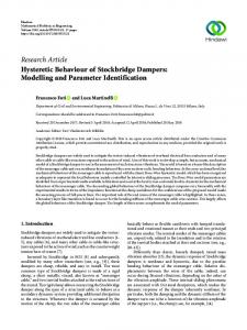
˙ w) is the output force of the MR damper, x(t) ˙ where Φn (x, and v are the velocity and voltage inputs, respectively. The voltage input v is the applied voltage at the coil of the MR damper. The system parameters, which are voltagedependent, are κx˙ (v) > 0, κw (v) > 0, ρ > 0, σ > 1/2, and n ≥ 1. These parameters control the shape of the hysteresis loop and their meaning can be found in [6]. The state variable w(t) has not a physical meaning so that it is not accessible to measurements. Since the normalized Bouc-Wen representation described in equations (1)-(2) is not a linear-in-parameter model, classical parameter identication methods cannot be applied. In this regard, a new parameter identication algorithm has been proposed in [7, p. 38], which is based on a physical understanding of the device along with a black box description. Rodr´guez et al. [17] used this methodology for a large-scale MR damper. The method is based on applying a periodic input velocity x(t) ˙ at a constant voltage coil v and observing the periodic steady-state force response of the MR damper. Nonetheless, large relative errors in the identication process can be observed when the MR damper has a viscous ˙ small enough with respect to the dry friction (κx˙ (v)x(t)) friction (κw (v)w(t)). To cope with this drawback, when the displacement is large enough, an alternative method based on the plastic region of the force-velocity diagram of the MR damper has been proposed in [16]. However, the model in equations (1)-(2) may not give an accurate representation of large-scale MR dampers which do not belong to the sheartype category. For instance, consider the black box model of an MR damper in the smart base-isolated benchmark building [13]. Figure 1 contains the force-displacement and force-velocity diagrams when this MR damper is excited by a sinusoidal displacement and velocity. In order to test the goodness of the Bouc––Wen model, this gure also contains the response of the dynamic model in equations (1)-(2) with some appropriate parameters. It can be observed that the resulting plastic branch in the force-velocity diagram is wider that the corresponding branch of the Bouc––Wen model. In the literature, the same type of cycles have been experimentally reported, for instance, in [4, Figure 4(b)], [11, Figure 9] and [12, Figure 7]. Therefore, it can be derived that this kind of hysteretic loops are unable to be reproduced with the original Bouc––Wen model. To improve the accuracy of the model representation and, consequently, the accuracy of the parameter identication, we use the following extended Bouc-Wen model: ˙ w)(t) = κx (v)x(t) + κx˙ (v)x(t) ˙ + κw w(t), Φe (x, x, n−1

w(t) ˙ = ρ(x(t) ˙ − σ|x(t)||w(t)| ˙ n + (σ − 1)x(t)|w(t)| ˙ ),

(3)

w(t) (4)

250

400

200

300

150

plastic branch

200

100 Force (kN)

(1)

˙ w)(t) = κx˙ (v)x(t) ˙ + κw (v)w(t), Φn (x,

where the term κx (v)x(t), which represents a linear elastic force, has been added. We consider that the coefcient κx is voltage-dependent, as the other parameters. The effect of this term can be observed not only in the force-velocity diagram, but also in the force-displacement: the resulting plot is inclined. This feature has also been experimentally reported in, for instance, [2, Figure 8], [11, Figure 9] and [12, Figure 7].

Force (kN)

[22]. For MR dampers in shear mode it takes the form:

50 0 −50

100 0 −100

−100 −200

−150

−300

−200 −250 −0.4

−0.2

0

Displacement (m)

0.2

0.4

−400 −2

−1

0

1

2

Velocity (m/s)

Fig. 1. Force-displacement (left) and force-velocity (right) diagrams of the black box model of the MR damper when it is excited by a sinusoidal displacement and velocity (dashed). The response of the dynamic Bouc–– Wen model in equations (1)-(2) under the same excitation is represented by a solid line.

III. MODEL PARAMETER IDENTIFICATION This section is concerned with the computation of the parameters of the extended model in equations (3)-(4). The proposed algorithm will be divided in two steps: (a) the estimation of the value of κx and (b) the estimation of the rest of the parameters based on the identication algorithm in [17]. At constant voltage, the computation of the parameter κx (v) can be performed graphically by considering the forcedisplacement diagram of the MR damper. When this device is excited by a sinusoidal displacement with a large enough amplitude, the average inclination of the resulting plot gives an estimation of this parameter. As an example, consider the black box model of an MR damper in the smart base-isolated benchmark building. When this MR damper is driven with zero coil command voltage, we obtain the force-displacement diagram in Figure 2 (left). The estimated value of κx is then computed as κx = 82.8 0.4 = 207 kN. To estimate the rest of the parameters, we use the knowledge of the parameter κx and the fact that ˙ w)(t) = Φe (x, x, ˙ w)(t) − κx (v)x(t). Φn (x, Figure 2 (right) depicts (in solid line) the force-velocity diagram for the resulting output force Φe of the MR damper minus the linear elastic force κx (v)x(t), when this device is excited by a sinusoidal displacement and velocity. It can be recognized from this gure that this new cycle has the same shape as the force-velocity cycle of the model in equations (1)-(2), which is plotted in Figure 1 right . As a result, for the identication of the rest of the parameters, that is, the

497

MoA14.4

A. Bahar et al.: Parameter Identification of Large-Scale Magnetorheological Dampers in a Benchmark Building Platform

parameters of the model Φn (x, ˙ w)(t) = κx˙ (v)x(t) ˙ + κw (v)w(t), n−1 w(t) ˙ = ρ(x(t) ˙ − σ|x(t)||w(t)| ˙ w(t) n ), + (σ − 1)x(t)|w(t)| ˙

we can follow basically the same idea as in [17]. The details of this method are omitted here but can be found in the Appendix.

B. Identication results In order to implement the identication procedure in Section II it is necessary to apply a periodic excitation displacement and observe the corresponding MR damper force. Figure 3 illustrates these two signals for a zero voltage. A set of experiments have been performed for different voltages in the range [0, 1] volts. 80

0.03

60

0.02

250

200

300

150

Force (kN)

Displacement (m)

40

400

0.01 0 −0.01

0 −20 −40

200 −0.02

82.8 kN

100 0

Force (kN)

100

Force (kN)

20

50

−0.03

−60 0

2

4

0

6

8

10

−80

0

2

4

Time (s)

6

8

10

Time (s)

−50

−100

−100

−200

Fig. 3. Response of the MR damper model in the benchmark building platform.

−150

−400 −0.5 −0.4 −0.3 −0.2 −0.1 0 0.1 0.2 Displacement (m)

−200

0.3

0.4

0.5

−250 −2

−1.5

−1

−0.5

0

0.5

1

1.5

2

Velocity (m/s)

Fig. 2. The average inclination of the force-displacement diagram, when the MR damper is excited by a sinusoidal displacement, gives an estimation of the parameter κx (left). Force-velocity diagram for the resulting output force Φe of the MR damper (dashed) and the force Φn = Φe − κx (v)x(t) (solid) (right).

This section is concerned with the application of the proposed method on a virtual MR damper. More precisely, the proposed identication algorithm is tested using a black box model of an MR damper, which is a part of a smart baseisolated benchmark building problem [13]. Consequently, we use this numerical platform as a virtual laboratory test. To validate the results, the output forces of the virtual device and the identied one will be compared using seven predened earthquake records of the benchmark problem with their corresponding uctuating voltage during full simulations. The MR damper is used in this context as a semi-active device to reduce the structural response of the building. A. Smart base-isolated benchmark building The smart base-isolated benchmark building [13] is employed as an interesting and more realistic example to further investigate the effectiveness of the proposed design approach. This benchmark problem is recognized by the American Society of Civil Engineers (ASCE) Structural Control Committee as a state-of-the-art model developed to provide a computational platform for numerical experiments of seismic control attenuation [14], [20]. The benchmark structure is an eight-storey frame building with steel-braces, 82.4 m long and 54.3 m wide, similar to existing buildings in Los Angeles, California. Stories one to six have an L-shaped plan while the higher oors have a rectangular plan. The superstructure rests on a rigid concrete base, which is isolated from the ground by an isolator layer, and consists of linear beam, column and bracing elements and rigid slabs. Below the base, the isolation layer consists of a variety of 92 isolation bearings. The isolators are connected between the drop panels and the footings below.

The resulting values of the parameters of the model in equations (3)-(4) are listed in Table I. Figure 5 plots these parameters as a function of the voltage. To nd an accurate voltage-dependent relation of these parameters, and according with the functional dependence in Figure 5, we consider that κx (v) is constant, κx˙ (v) is linear and n(v), ρ(v) and σ(v) are exponential: κx (v) = κx

(5)

κx˙ (v) = κx,a ˙ + κx,b ˙ v n(v) = na + nb exp(−13v)

(6) (7)

ρ(v) = ρa + ρb exp(−14v) σ(v) = σa + σb exp(−14v)

(8) (9)

Because of the importance of the parameter κw due to its great inuence in the resulted force (the range of its magnitude is, approximately, from 50 kN to 1000 kN, as can be seen in Table I), its voltage dependence function has been estimated in three different regions based on the variation of the resulted values (Figure 4). 1200

1000

κw6 + κw7 v +κw8 v 3 + κw9 v 5

800

κw

−300

κw3 + κw4 sin( π(v−0.3) ) 0.8 ) +κw5 sin( 3π(v−0.3) 0.8

600

400

200

0

κw1 + κw2 v 1.15 0

Fig. 4.

0.1

0.2

0.3

0.4

0.5 Voltage (V)

0.6

0.7

0.8

0.9

1

Results of the parameter identication algorithm.

The coefcients κx,a ˙ , κx,b ˙ , κw1 , . . . , κw9 , na , nb , ρa , ρb , σa and σb , which are listed in Table II, can be computed using

498

MoA14.4

Proceedings of the European Control Conference 2009 • Budapest, Hungary, August 23–26, 2009

TABLE II

208

κx

207.5

I DENTIFICATION RESULTS

207

206.5 206

0

0.1

0.2

0.3

0.4

0.5 Voltage (V)

0.6

0.7

0.8

0.9

1

parameter

400

value

κx˙

300

κx

200

κx,a ˙ κx,b ˙ ρa ρb na nb σa σb κw1 κw2 κw3 κw4 κw5 κw6 κw7 κw8 κw9

100 0

0

0.1

0.2

0.3

0.4

0.5 Voltage (V)

0.6

0.7

0.8

0.9

κx˙

1

1500

κw

ρ

1000 500 0

n 0

0.1

0.2

0.3

0.4

0.5 Voltage (V)

0.6

0.5 Voltage (V)

0.6

0.7

0.8

0.9

1

σ

1.47

n

1.46 1.45 1.44 1.43

0

0.1

0.2

0.3

0.4

0.7

0.8

0.9

1

ρ

650

κw

648 646 644

0

0.1

0.2

0.3

0.4

0.5 Voltage (V)

0.6

0.7

0.8

0.9

1

0

0.1

0.2

0.3

0.4

0.5 Voltage (V)

0.6

0.7

0.8

0.9

1

0.78

σ

0.775

207 89.64 292 648.95 −3.86 1.44 0.02 0.76 0.009 55.38 2270.0 619.85 387.34 18.42 −87.52 2665.0 −3054.7 1545.5

0.77 0.765 0.76

Fig. 5.

Results of the parameter identication algorithm.

MATLAB. The voltage-dependent functions are plotted in Figure 5.

dition using, for instance, an earthquake record and the corresponding uctuating command voltage as a consequence of the control process. To do this, our identied model is compared with the corresponding black box model of the MR damper in the benchmark building platform under exactly the same situation. To measure the discrepancy between the two models, the 1-norm error (ε) is used:

TABLE I I DENTIFICATION RESULTS

v 0.00 0.05 0.10 0.15 0.20 0.25 0.30 0.35 0.40 0.45 0.50 0.55 0.60 0.65 0.70 0.75 0.80 0.85 0.90 0.95 1.00

κx 207 207 207 207 207 207 207 207 207 207 207 207 207 207 207 207 207 207 207 207 207

κx˙ 89.643 104.24 118.84 133.44 148.04 162.64 177.24 191.84 206.44 221.04 235.64 205.25 264.84 279.44 294.04 308.64 323.24 337.84 352.44 367.04 381.64

κw 54.652 125.97 214.49 313.47 416.96 519.87 617.94 707.73 786.63 852.86 905.48 944.37 970.24 984.64 989.94 989.34 986.89 987.43 996.67 1021.1 1068.2

ρ 644.92 647.34 648.11 648.45 648.64 648.75 648.82 648.87 648.90 648.92 648.94 648.95 648.96 648.96 648.96 648.96 648.96 648.96 648.96 648.96 648.98

#FBM − Fid #1 , #FBM #1 ! Tr #f #1 = |f (t)|dt, ε=

n 1.4557 1.4436 1.4398 1.4381 1.4372 1.4366 1.4362 1.4360 1.4358 1.4357 1.4357 1.4356 1.4356 1.4355 1.4355 1.4355 1.4355 1.4355 1.4355 1.4355 1.4355

σ

(10) (11)

0

0.7733 0.7674 0.7656 0.7648 0.7643 0.7641 0.7639 0.7638 0.7637 0.7636 0.7636 0.7636 0.7636 0.7636 0.7636 0.7636 0.7636 0.7636 0.7638 0.7636 0.7635

where FBM is the output force of the black box model (benchmark building platform) and Fid is the resulting force of the identied MR damper based on the model in equations (3)-(4). The length in time of each earthquake is denoted by Tr . The 1-norm is a measure that reects the average size of a signal and thus it is a good tool for computing the discrepancy between these two models. Based on this 1-norm, if the computed value of the damping force is far from the reference value, the value of ε will be large. On the contrary, if it is small, the identied model can produce forces which are very close to real ones. Table III presents the model errors for several earthquakes (FP-x and FP-y are the estimation errors in the x-force and y-force directions). A sample earthquake record and the corresponding command voltage during the control process are presented in Figure 6. In this application, the MR damper is used as a semi-active device in which the voltage is varying by a feedback control loop [8].

C. Model validation The identication models presented in the literature usually have good accuracy when they consider a constant voltage. However, because of the role of MR dampers as a semi-active devices in structural control systems, the nal identied model has to be checked under a simulated con-

D. Comparison of results It is interesting to compare the resulting model errors in Table III with the resulting model errors when the parameter identication is performed with the model in equations (1)(2). Table IV shows the values of the errors for this case.

499

MoA14.4

300

1500

200

1000 Damper Force (kN)

Ground Acceleration (m/s^2)

A. Bahar et al.: Parameter Identification of Large-Scale Magnetorheological Dampers in a Benchmark Building Platform

100 0 −100 −200

−1500

0

5

10

15 Time (s)

20

25

5

10

15 Time (s)

20

25

30

0

5

10

15 Time (s)

20

25

30

1500

Damper Force (kN)

1000

0.8

Voltage

0

30

1

0.6 0.4

500 0 −500 −1000 −1500

0.2 0

0 −500 −1000

−300 −400

500

0

5

10

15 Time (s)

20

25

30

Fig. 6. El Centro, ground acceleration (top) and corresponding command voltage (bottom).

Fig. 7. Comparison of the MR damper force for the proposed model (top/solid) and for the model in [16] (bottom/solid), both with the response of the original black box model (dashed), under Kobe ground motion (FP-y). 1000

TABLE III Damper Force Error (kN)

E RROR NORM (ε) FOR THE PROPOSED PARAMETER IDENTIFICATION

Newhall

Sylmar

El Centro

500

0

−500

Rinaldi −1000

6.47% 3.84%

5.67% 8.44%

7.78% 7.90%

FP-x FP-y

Kobe

Jiji

Erzinkan

6.52% 7.85%

3.61% 4.02%

4.88% 5.35%

7.12% 5.67%

E RROR NORM (ε) FOR THE METHOD IN [16]

FP-x FP-y FP-x FP-y

Sylmar

El Centro

Rinaldi

16.15% 15.83%

18.06% 24.14%

22.89% 19.68%

17.55% 18.48%

Kobe

Jiji

Erzinkan

18.22% 24.72%

14.16% 20.09%

14.91% 18.80%

5

10

15 Time (s)

20

25

30

0

5

10

15 Time (kN)

20

25

30

500

0

−500

−1000

TABLE IV

Newhall

0

1000 Damper Force Error (kN)

FP-x FP-y

Fig. 8. Generated damper force errors for proposed model (above), and original method [16] (below) , under Kobe ground motion (FP-y).

of the parameter identication method has been tested using the MR damper as a semi-active device under time-varying voltage and earthquake excitation. A PPENDIX

By comparing these two tables, the proposed parameter identication algorithm is clearly more accurate than the method presented in [16]. Figure 7 shows the comparison between the output force of the black box MR damper during the simulation of the benchmark building under Kobe earthquake, with the two identied models, the proposed one and the model in [16]. Since the two plots in Figure 7 (top) are very close, Figure 8 shows the corresponding errors in both cases. IV. C ONCLUSION This paper has proposed an extension of a parameter identication method for MR dampers. This extension allows to identify a larger class of MR dampers more accurately. The validation of the parameter identication method has been carried out using a black box model of an MR damper in a smart base-isolated benchmark building. The versatility

The parameter identication in [17] departs from the next shear-mode model: (12)

˙ = κx˙ (v)x(t) ˙ + κw (v)w(t) Φn (x)(t) n−1

w(t) ˙ = ρ(x(t) ˙ − σ|x(t)||w(t)| ˙ n ) + (σ − 1)x(t)|w(t)| ˙

w(t) (13)

where κx > 0, κw > 0, ρ > 0, σ > 1/2, and n ≥ 1. For parameter identication, a T -periodic input x(t) ˙ (see Figure 9) is applied to the Bouc-Wen system under constant voltage v. It has been proved [7] that the output force of the Bouc-Wen model goes asymptotically to a periodic steadystate so that a limit cycle is obtained. The identication method assumes the knowledge of the relation w(x) ¯ that describes this cycle. The whole identication process can be summarized as follows. The parameter κx˙ is rst determined using the plastic region (w ¯ ≈ 1) of the hysteresis loop by a linear regression

500

MoA14.4

Proceedings of the European Control Conference 2009 • Budapest, Hungary, August 23–26, 2009

R EFERENCES

Input signal x

Xmax

Xmin T+

0

Fig. 9.

T

+ mT + T(m + 1)T

mT Time

A sample T -wave periodic signal

for each constant voltage: F¯ (τ ) = κx (v)x(τ ˙ ) + κw (v). To continue with parametric estimation, a function θ is computed as: dx(τ ) , τ ∈ [0, T + ], (14) θ(x(τ )) = F¯ (x(τ )) − κx˙ dτ which has a unique zero, i.e, there exists a time instant τ∗ ∈ [0, T +], and a corresponding value x∗ = x(τ∗ ) ∈ [Xmin , Xmax ], such that the function θ is zero. Because θ is known, then x˙ ∗ is also known. Dene the quantity " # dθ(x) a= . (15) dx x=x∗ Then, the parameter n is determined as: % $ dθ(x) −a ( dx ) log dθ(x) x=x∗2 ( dx )x=x∗1 −a ' & n= θ ∗2 log θx=x x=x

(16)

∗1

where x∗2 > x∗1 > x∗ are design parameters. Dene & ' a − dθ(x) dx x=x∗2 b= . θ(x∗2 )n

(17)

Then, the parameters κw and ρ are computed as follows: ( a (18) κw = n , b a . (19) ρ= κw The function w(x) ¯ can be computed as: θ(x) . κw Finally, the remaining parameter σ is determined as:  dw(x)  ( ¯dx )x=x∗3 − 1 1  ρ σ=  + 1 2 (−w(x ¯ ∗3 )n ) w(x) ¯ =

(20)

(21)

[1] G. Bossis , P. Khuzir, S. Lacis, and O. Volkova, Yield behavior of magnetorheological suspensions, Journal of Magnetism and Magnetic Materials, 258-259:456-458, 2003. [2] W.W. Chooi, S.O. Oyadiji, Design, modelling and testing of magnetorheological (MR) dampers using analytical ow solutions, Computers & Structures, 86(3-5):473––482, 2008. [3] A. Dominguez, R. Sedaghati, and I. Stiharu, Modeling and application of MR dampers in semi-adaptive structures, Computers & Structures, 86(3-5):407––415, 2008. [4] S.J. Dyke, B.F. Spencer Jr., M.K. Sain, and J. D. Carlson, An experimental study of MR dampers for seismic protection, Smart Materials and Structures, 7(5):693––703, 1998. [5] Z.Q. Gu, and S.O. Oyadiji, Application of MR damper in structural control using ANFIS method, Computers & Structures, 86(3-5):427–– 436, 2008. [6] F. Ikhouane, J.E. Hurtado, and J. Rodellar, Variation of the hysteresis loop with the Bouc-Wen model parameters, Nonlinear Dynamics, 48(4):361––380, 2007. [7] F. Ikhouane, and J. Rodellar, Systems with Hysteresis: Analysis, Identication and Control Using the Bouc-Wen Model, John Wiley & Sons, Inc., 2007. [8] L.M. Jansen, and S.J. Dyke, Semiactive control strategies for MR dampers: comparative study, Journal of Engineering Mechanics, 126(8):795––803,2000. [9] M. R. Jolly, J. W. Bender, and J. D. Carlson, Properties and applications of commercial magnetorheological uids, Journal of Intelligent Material Systems and Structures, 10(1):5––13,1999. [10] J. Gang, M. K. Sain, K. D. Pham, B. F. Spencer Jr., and J. C. Ramallo, Modeling MR dampers: A nonlinear black box approach, Proceedings of the American Control Conference: 429––434, 2001. [11] H. Gavin, J. Hoagg, and M. Dobossy, Optimal design of MR dampers, Proceedings of the US-Japan Workshop on Smart Structures for Improved Seismic Performance in Urban Regions, Seattle WA, 225–– 236, 2001. [12] G. Jin, M. K. Sain, and B. F. Spencer Jr., Nonlinear blackbox modeling of MR-damper for civil structural control, IEEE Transactions on Control Systems Technology, 13(3):345––355, 2005. [13] S. Narasimhan, S. Nagarajaiah, E. A. Johnson, and H. P. Gavin, Smart base-isolated benchmark building. Part I: Problem denition, Structural Control and Health Monitoring, 13(2-3):573––588, 2006. [14] Y. Ohtori, R.E. Christenson, B.F. Spencer and S.J. Dyke, Benchmark problems in seismically excited nonlinear buildings. Journal of Engineering Mechanics, 130(4):366––385, 2004. [15] F. Pozo, L. Acho, A. Rodr´guez, and G. Pujol, Nonlinear modeling of hysteretic systems with double hysteretic loops using position and acceleration information, Nonlinear Dynamics, doi: 10.1007/s11071008-9414-7. [16] A. Rodr´guez, F. Ikhouane, J. Rodellar, and N. Luo, Modeling and identication of a small-scale magnetorheological damper, Journal of Intelligent Material Systems and Structures, doi: 10.1177/1045389X08098440. [17] A. Rodr´guez, N. Iwata, F. Ikhouane, and J. Rodellar, Model identication of a large-scale magnetorheological uid damper, Smart Materials and Structures, 18(1), doi: 10.1088/0964-1726/18/1/015010, 2009. [18] S. M. Savaresi, S. Bittanti, and M. Montiglio, Identication of semiphysical and black box nonlinear models: The case of MR dampers for vehicles control, Automatica, 41(1):113––127,2005. [19] B. F. Spencer Jr., S. J. Dyke, M. K. Sain, and J. D. Carlson, Phenomenological model of a magnetorheological damper, Journal of Engineering Mechanics, 123(3): 230––238, 1997. [20] B.F. Spencer, and S. Nagarajaiah, State of the art of structural control. Journal of Structural Engineering, 129(7):845––856, 2003. [21] D. H. Wang, and W. H. Liao, Neural network modeling and controllers for magnetorheological uid dampers, Proceedings of the 10th IEEE International Conference on Fuzzy Systems, 3: 1323––1326, 2001. [22] Y. K. Wen, Method for random vibration of hysteretic systems, Journal of Engineering Mechanics, 102(2):249-263, 1976. [23] P.Q. Xia. An inverse model of MR damper using optimal neural network and system identication, Journal of Sound and Vibration, 266(5):1009-1023, 2003.

where x∗3 is a design parameter such that x∗3 < x∗ .

501