Parameterised Sigmoid and ReLU Hidden Activation Functions for ...

INTERSPEECH 2015

Parameterised Sigmoid and ReLU Hidden Activation Functions for DNN Acoustic Modelling C. Zhang & P. C. Woodland Cambridge University Engineering Dept., Trumpington St., Cambridge, CB2 1PZ U.K. {cz277,pcw}@eng.cam.ac.uk

Abstract

that on LVCSR tasks with very large training sets, pre-training for even Sigmoid DNNs is unnecessary [11], the above findings still illustrated the importance of hidden activation functions. Recently, there have been several studies on learning parameterised activation functions [12, 13, 14]. In [12], Hermite polynomial activation functions with a number of coefficients are learnt in a speaker independent (SI) ANN acoustic model, and the coefficients are made speaker dependent (SD) by adapting to a particular speaker during testing. Similarly, [13] associates each hidden unit with a weight constraint by Sigmoid functions, and the DNN is adapted by learning the hidden unit contributions (LHUC). An advantage of LHUC is that it does not rely on the choice of hidden activation functions. The parametric leaky ReLU1 (PLReLU) was proposed as a general activation function, and applied to a 22-layer convolutional neural network for image classification [14]. The PLReLU has the coefficients of its negative part adaptively learned and allows an automatic learning of rectification. In this paper, we study the parameterised forms of the most commonly used hidden activation functions – Sigmoid and ReLU. Three parameters are used with the generalised Sigmoid: the curve’s maximum value, the curve’s steepness, and a scaled horizontal displacement. In this way, the parameterised Sigmoid function can perform piecewise approximations to other activation functions. Meanwhile, both positive and negative parts of ReLU are separately associated with a linear scaling factor, which allows unconstrained trade-off between the positive and negative activations. We investigate the effectiveness and the role of these parameters in training standard DNN acoustic models. Section 2 briefly reviews the common DNN training algorithm. The training method and properties of each parameter are discussed in Section 3. The experimental setup is presented in Section 4, followed by the experimental results in Section 5, and conclusions are presented in Section 6.

The form of hidden activation functions has been always an important issue in deep neural network (DNN) design. The most common choices for acoustic modelling are the standard Sigmoid and rectified linear unit (ReLU), which are normally used with fixed function shapes and no adaptive parameters. Recently, there have been several papers that have studied the use of parameterised activation functions for both computer vision and speaker adaptation tasks. In this paper, we investigate generalised forms of both Sigmoid and ReLU with learnable parameters, as well as their integration with the standard DNN acoustic model training process. Experiments using conversational telephone speech (CTS) Mandarin data, result in an average of 3.4% and 2.0% relative word error rate (WER) reduction with Sigmoid and ReLU parameterisations.

1. Introduction Multi-layer perceptrons (MLPs) have become a widely used artificial neural network (ANN) model since the rediscovery of the error back propagation (EBP) algorithm in the 1980s [1, 2]. However, it was commonly believed that training a DNN, an MLP with many hidden layers, directly from random initialisations using EBP usually gives to a poor local optimum [3]. The problem had not been addressed until a generative pre-training approach was proposed to initialise the DNN with Sigmoid activation functions layer by layer, by training a stacked set of unsupervised RBMs [4]. Studies on image classification tasks found one perspective to understand the difficulty in deep learning: the non zero mean value of the Sigmoid function drives the top hidden layer of a random initialised DNN into saturation, while other non-linear functions symmetric around zero with sensible random initial values can enable DNNs to converge to a good local optimum quickly without pre-training [3]. In 2010, a half-rectified non-linearity, the rectified linear unit or ReLU, which is linear for positive values and zero otherwise, was studied [5, 6] and applied to large vocabulary continuous speech recognition (LVCSR) [7, 8]. Compared to Sigmoid, ReLU can usually eliminate the necessity of pre-training and make DNNs converge to sometimes more discriminative solutions more quickly, while keeping the model sparse [5, 7, 8]. A further improvement of the ReLU is the leaky ReLU, which scales the negative part by 0.01, to allow small non-zero gradients when a unit is saturated [9]. However, it results in no improvement in speech recognition [9, 10]. Although it was found

2. A Review of DNNs 2.1. DNN-HMM Hybrid Acoustic Models An MLP maps its input vector xt to an output vector through the nodes in the hidden and output layers. xt is formed from a stacked set of adjacent frames of the acoustic feature vector, ot , for each frame. A DNN is an MLP with many hidden layers. In each layer, the input to each node j, aj , is defined as a weighted sum of the outputs from its previous layer, yi , i.e., X aj = wji yi + bj , (1)

Chao Zhang is supported by Cambridge International Scholarship from the Cambridge Commonwealth, European & International Trust and by the EPSRC Programme Grant EP/I031022/1 (Natural Speech Technology). Supporting data for this paper is available at the http://www.repository.cam.ac.uk/handle/1810/248386 data repository.

Copyright © 2015 ISCA

i 1 The

3224

method was denoted the parametric ReLU (PReLU) in [14]

September 6- 10, 2015, Dresden, Germany

where wji and bj are the weights and bias associated with node j, and aj is also called the activation. Node j transforms its input aj with an activation function fj (·),

In this section, we study a generalised form of Sigmoid, f (a) = η ·

yj = fj (aj ).

3.1.1. Properties of the p-Sigmoid In the p-Sigmoid function, η, γ, and θ have different effects on the curve f (a). • Among the three parameters, η can make the largest change to the function by scaling f (a) linearly. |η| is the maximum value of |f (a)|. Since we impose no constraint on the parameters, η can be any real number. If η > 0, η indicates the contribution of the relevant hidden unit, which can be seen as a case of LHUC [13]; the unit is disabled if η = 0. We enable the units to make negative contributions by allowing η < 0.

ln p(xt |sk ) = ln(sk |xt ) + ln p(xt ) − ln P (sk ), P0 where P (sk ) = Tk / k Tk0 , Tk is the number of frames labeled as sk , and p(xt ) is independent of the HMM state.

• γ controls the steepness of the curve. When |γ| increases, f (a) can arbitrarily approximate a step function. When γ → 0, f (a) makes less difference to the input around 0, and outputs constant values if γ = 0.

2.2. Training DNNs with Error Backpropagation When updating DNN parameters using stochastic gradient descent (SGD) according to some objective function F, the first step is to compute the derivatives of F with respect to every parameter, ϕi , which is associated with node i. If ϕi is a weight or bias, then according to the chain rule,

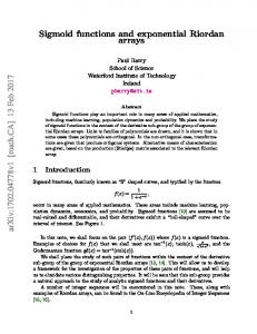
• θ applies a horizontal displacement to f (a). θ/γ is the x-value of the midpoint of the p-Sigmoid, if γ is nonzero. It is well-known that the p-Sigmoid, or logistic function, can be used for piecewise approximations to other functions. Fig. 1 illustrates different shapes of p-Sigmoid for a ∈ [−5, 5], by varying η, γ, and θ. p-Sigmoid(1, 30, 0) is similar to the standard threshold activation function [2]. The illustrated fragment of p-Sigmoid(4, 1, 2) has a similar shape as that of the Soft ReLU activation function [5, 10]. p-Sigmoid(3, −2, 3) approximates ReLU, although the approximation is poor around zero. Therefore, if all parameters are learnt properly, many pSigmoid units can behave as several commonly used activation functions. Therefore, we associate each hidden unit activation function fi (ai ) with a set of parameters, ηi , γi , and θi .

(2)

it relies on ∂F/∂ai . Again, applying the chain rule, we obtain ∂F ∂yi X ∂F ∂aj = ∂ai ∂ai j ∂aj ∂yi =

∂fi (ai ) X ∂F wji , ∂ai ∂aj j

(3)

which is computed based on ∂F/∂aj propagated back from the next layer. If ϕi ∈ Φi is a parameter of the activation function fi (·), assume ϕi is not shared by different functions, then

3 f (a) p-Sigmoid(1, 1, 0)

∂F ∂yi X ∂F ∂aj = ∂ϕi ∂ϕi j ∂aj ∂yi =

∂fi (ai ) X ∂F wji . ∂ϕi ∂aj j

(5)

which is actually the logistic function, and η, γ, and θ are the learnable parameters. We denote Eqn. (5) as defining the pSigmoid(η, γ, θ).

If it is a hidden layer and fj (·) has no adaptive parameters, fj (·) is a standard activation function, (e.g., Sigmoid or ReLU). Otherwise fj (·) is a parameterised function with a set of learnable parameters, Φj . In the output layer, the inputs to node k, ak , are normalised to be the posterior probability of its associated class Ck , using the softmax function fk (·). To interface a DNN with HMMs, the posterior probability p(Ck |xt ) is converted to a scaled loglikelihood of xt generated by sk , the HMM state relevant to Ck , by

∂F ∂F ∂ai = , ∂ϕi ∂ai ∂ϕi

1 , 1 + e−γa+θ

p-Sigmoid(1, 30, 0)

2

p-Sigmoid(4, 1, 2) p-Sigmoid(3, -2, 3)

(4)

If F is the cross entropy (CE) criterion, ∂FCE /∂ak = yk − yˆk , where yˆk is the reference of Ck at time t. yk − yˆk acts as the error backpropagated by Eqns. (2)–(4) to compute the gradients for all parameters. Therefore, the algorithm is usually referred to as error backpropagation (EBP) [2].

p-Sigmoid(2, 2, 0) -1

1

-3

0

a

-5

-4

-2

-1

1

2

3

4

5

-1

3. Parameterised Activation Functions Figure 1: Piecewise approximation by p-Sigmoid functions.

3.1. Parameterised Sigmoid Function

Note that p-Sigmoid(2, 2, 0)−1.0 is the hyperbolic tangent activation function [2], as drawn with the dashed line in Fig. 1. However, we do not allow a learnable parameter of p-Sigmoid to control the vertical shift since it can be acquired by changing the biases of the next layer.

Functions from the Sigmoid family have been widely investigated for many ASR tasks. For example, activation functions for ANN models [15, 16], smoothed forms of 0-1 classification error [17], and for making soft decisions on data selection according to noise estimation error [18].

3225

3.1.2. Implementing p-Sigmoid

scaling up ReLU outputs may cause gradient explosion [19], it is also possible that the automatically learnt scaling factors can prevent explosion occurring by scaling down ReLU outputs. In addition, for p-ReLU functions, even if the gradient does get too large, this issue can be fixed using simple gradient clipping [20] and ReLU output value clipping methods.

From Eqns. (2)–(4), it is necessary to compute the partial derivatives of fi (·) with respect to its input activation ai , and also to each of its parameters ηi , γi , and θi . For the p-Sigmoid, the derivatives are computed by  ∂fi (ai ) 0
if ηi = 0 , (6) = γi fi (ai ) 1 − ηi−1 fi (ai ) if ηi 6= 0 ∂ai  ∂fi (ai ) (1 + e−γi ai +θi )−1 if ηi = 0 , (7) = ηi−1 fi (ai ) if ηi 6= 0 ∂ηi  ∂fi (ai ) 0
if ηi = 0 , (8) = ai fi (ai ) 1 − ηi−1 fi (ai ) if ηi 6= 0 ∂γi  ∂fi (ai ) 0 if ηi = 0
= . (9) −fi (ai ) 1 − ηi−1 fi (ai ) if ηi 6= 0 ∂θi

4. Experimental Setup The experiments presented below were conducted with systems trained on 72 hours of Mandarin CTS data, denoted rt04train, which contains 50 hours of LDC 2004 CTS Mandarin data, as well as 22 hours from the LDC Call Home Mandarin and Call Friend Mandarin data sets. The training set consists of 786 conversational sides, and was used in building the 2004 Cambridge University HTK-based Mandarin system. Three test sets were used: a 2 hour development set dev04 containing 24 conversations associated with rt04train; the 2003 NIST evaluation set, eval03, which includes 1.1 hours of data from 12 conversations from the Call Friend corpus; as well as 1997 NIST Hub5 Mandarin evaluation set, eval97, which contains 1.5 hours of data from 20 conversations. The recognition word list contains 63k words, comprising about 52k multi-character Chinese words, 5k single character Chinese words, and an additional 5k frequent English words. The base phone set contains 46 toneless phones or 124 total phones. Decoding was performed with a bigram langauge model (LM) and the generated lattices were rescored with an interpolated trigram back-off LM. Both LMs were trained using a total of 1 billion words of text data. All results presented in Section 5 are with a trigram LM. More details about the dictionary and LMs can be found in [21]. The acoustic feature vector uses 13d PLP coefficients with their ∆, ∆∆, and ∆∆∆, normalised by vocal tract length normalisation (VTLN) and projected to 39d using HLDA [22, 23]. VTLN was used in supervised and unsupervised modes on the training and testing data, respectively. Pitch features extracted by the Kaldi toolkit [24, 25], along with their ∆ and ∆∆ were appended to the projected vector. The 42d augmented vector was further normalised by cepstral mean and variance normalisation (CMN and CVN) at the speaker level, and then used to build SD GMM-HMMs for CMLLR transform estimation. After transformation by CMLLR, the feature vector was normalised again to zero mean and unit variance. Finally, the current frame of this 42d speaker normalised feature vector, was concatenated with 4 frames to its left and right, respectively, which formed the final 378d DNN input feature vector. The DNN training alignments were generated by a Tandem SAT system. The DNN output targets were derived from a tonal triphone context-dependent GMM-HMM system with 6005 tied states, clustered with the phonetic decision tree state tying approach [26]. More details about the tonal GMM-HMMs and the Tandem SAT system can also be found in [21]. All DNNs had 5 hidden layers with 1000 nodes per layer and were trained based on the CE criterion. Therefore, the structure for all DNNs used as DNN-HMMs was 378 × 10005 × 6005. For the purpose of cross-validation, 10% of rt04train was randomly selected at the speaker level and held out of training. Parameter updates were averaged over a mini-batch with 800 frames and smoothed by adding a “momentum” term of 0.5 times the previous updates. A modified NewBob algorithm described in [27] was used as the learning rate scheduler. For DNNs with Sigmoid and p-Sigmoid activation functions, the initial learning rate η0 and minimum epoch number Nmin were

From Eqns. (7) and (8), the input activation, ai , needs to be used in computing the gradients. This is a different requirement to the Sigmoid function, where ai does not need to be kept for EBP, and it gives rise to extra cost for both computation and storage. The computational cost is negligible if a GPU is used in training. Furthermore, when γi is not involved in training, we have found that using ∂fi (ai )/∂ηi = 0 for the ηi = 0 case in Eqn. (7) makes only a little difference2 , which can simplify the implementation. 3.2. Parameterised ReLU Function For the ReLU function with a hinge-like shape, the most straightforward way to make it into a parameterised form is to individually associate a scaling factor with either part of the function. i.e., to enable the two ends of the hinge to rotate separately around the “pin”. We denote this function p-ReLU as,  α · a if a > 0 f (a) = , (10) β · a if a 6 0 where α, and β are real-valued scaling factors of the positive and negative parts. The PLReLU proposed in [14] is a simplified form of p-ReLU(α, β), by fixing α = 1. Similarly, another simplified form of interest is p-ReLU(α, 0). In a similar way to the p-Sigmoid, the function parameters depend on each hidden node i. Therefore, the derivatives of p-ReLU with respect to a, αi , and βi for EBP are  ∂fi (ai ) αi if ai > 0 = , (11) βi if ai 6 0 ∂ai  ∂fi (ai ) ai if ai > 0 = , (12) 0 if ai 6 0 ∂αi  ∂fi (ai ) 0 if ai > 0 = . (13) ai if ai 6 0 ∂βi Since the values of αi and βi are not constrained, the sign of ai cannot be inferred from fi (ai ). Therefore it is necessary to keep ai for backpropagation which results in extra memory usage. As for the p-Sigmoid case, for p-ReLU(αi , 0), ai does not need to be kept by not updating the zero-valued αi . Moreover, it may be argued, for unbounded activation functions like ReLU, scaling its value with a factor with absolute values bigger than 1 is unsafe. However, in our experiments, it was not found to cause any issues. This indicates, that while 2 Note that this approximation was not used in the experiments reported in this paper.

3226

set to 2.0 × 10−3 and 12. Discriminative pre-training [28, 15] was used for sigmoidal DNNs, which trains the model for 1 epoch every time a new layer is stacked. For DNNs with ReLU and p-ReLU functions, 5.0 × 10−4 and 8 were used as η0 and Nmin . The DNN, which produced the highest held-out set frame classification accuracy in fine-tuning, was used as the final model. All GMM-HMMs and DNN-HMMs acoustic model training and decoding used HTK [29, 27].

the negative rather than the positive part to be recified in ReLU. In summary, it is found helpful to keep the p-Sigmoid parameters frozen at the begining of training, but uncessary or even harmful for p-ReLU systems. 5.2. Which p-Sigmoid and p-ReLU Parameters to Train DNN-HMMs with other choices of p-Sigmoid and p-ReLU functions are shown in Table 2. From the results, none of the pSigmoid and p-ReLU systems with multiple learnt parameters has outperformed S1 and R1, which are the best two systems with only the linear scaling factors estimated.

5. Experimental Results We investigated the use of p-Sigmoid and p-ReLU for standard DNN acoustic model training. All CD-DNN-HMMs were constructed following the configurations described in Section 4. The initial value of all ηi , γi , θi , αi , and βi were set to be 1.0, 1.0, 0.0, 1.0, and 0.25, if not explicitly defined. There are two key things of interest: which activation function parameters to select and how to train these parameters properly. For clarity, we only present dev04 results in subsection 5.1.

ID R1 R2 R3 R1− R2−

5.1. How to train p-Sigmoid and p-ReLU Parameters

Activation Function p-Sigmoid(ηi , 1, 0) p-Sigmoid(1, γi , 0) p-Sigmoid(1, 1, θi ) p-Sigmoid(ηi , 1, 0) p-Sigmoid(1, γi , 0) p-Sigmoid(1, 1, θi ) p-Sigmoid(ηi , γi , 0) p-Sigmoid(1, γi , θi ) p-Sigmoid(ηi , 1, θi ) p-Sigmoid(ηi , γi , θi )

dev04 26.8 27.0 27.1 27.4 27.0

Table 2: dev04 %WER for the p-ReLU systems. − indicates the activation function parameters were frozen in the 1st epoch.

For the p-Sigmoid systems, care needs to be taken in training the activation function parameters from the pre-training (PT) step, since some parameters, e.g., ηi , can change the p-Sigmoid outputs rapidly and can affect the convergence of the other model parameters. Starting to train p-Sigmoid parameters from the fine-tuning (FT) step is preferred since all weights and biases are already sensibly initialised. Therefore, we first compare training ηi , γi , and θi individually in both PT and FT, and FT only. The results are listed in Table 1. ID S1+ S2+ S3+ S1 S2 S3 S4 S5 S6 S7

Activation Function p-ReLU(αi , 0) p-ReLU(1, βi ) p-ReLU(αi , βi ) p-ReLU(αi , 0) p-ReLU(1, βi )

Full results on the 3 testing sets are presented in Table 3. S0 and R0 are the baseline systems with standard Sigmoid and ReLU functions. Comparing S1 to S0, R1 to R0, p-Sigmoid and p-ReLU resulted in on average 3.4% and 2.0% relative WER reduction, by increasing only 0.06% parameters (6,000 among 10,394,005) in training, which illustrates the important role of parameterised activation functions. Of course, an equivalent model without any activation function parameters can be obtained by replacing the p-Sigmoid(ηi , 1, 0) or p-ReLU(αi , 0) with Sigmoid or ReLU, and scaling the relevant weights of the next layer by ηi or αi . Furthermore, although on this task, p-ReLU outperformed p-Sigmoid, the relative improvement is smaller. This shows that the improvement from p-Sigmoid may already contain some benefits from making the Sigmoid more similar to ReLU using ηi , but more improvements were from the extra flexibility to allow the contribution of each hidden unit to be automatically and individually weighted.

dev04 27.6 27.7 27.7 27.1 27.5 27.4 27.2 27.2 27.4 27.3

ID S0 S1 R0 R1

Table 1: dev04 %WERs for the p-Sigmoid systems. + means the activation function parameters were trained in both PT and FT. Comparing S1+ , S2+ , and S3+ to S1, S2, and S3 respectively, we can see all p-Sigmoid systems that start to learn their parameters from FT outperformed their counterparts that learn all the parameters together since PT. These results coincide with our above mentioned inference. Meanwhile, we also tested this idea with the p-ReLU systems. Since we did not use PT for training ReLU DNNs, the p-ReLU parameters were kept fixed in the first epoch to avoid them affecting the other parameters. The resulted systems are R1− and R2− . From Table 2, it is clear that training αi from the first epoch makes R1 outperform R1− , while doing this for βi makes no impact on WERs. This reveals two things: first, since ReLU DNNs have unbounded activation functions, their parameters can be more robust to the fluctuation of the activation function outputs, and it is not useful to avoid the impact on the other parameters at the begining; second, αi has more impact on training than βi , which supports

Activation Function Sigmoid p-Sigmoid(ηi , 1, 0) ReLU p-ReLU(αi , 0)

eval97 34.1 32.9 33.3 32.7

eval03 29.7 28.6 29.1 28.7

dev04 27.9 27.1 27.6 26.8

Table 3: %WER on all test sets.

6. Conclusions In this paper, the use of general parameterised forms of Sigmoid and ReLU activation functions was studied. It was found that a linear scaling factor with no constraint imposed is the most useful for both Sigmoid and ReLU. Experimental results on a challenging CTS Mandarin task showed that DNNs trained with parameterised Sigmoid and ReLU functions resulted in, respectively, 3.4% and 2.0% relative reductions in WER. This reduction in WER requires an increase in the number of parameters in training by only 0.06% and if the linear activation function scalings are converted to scaling the following layer weights, then no extra parameters in the final model are required.

3227

7. References

[17] B.-H. Juang, W. Chou, and C.-H. Lee, “Minimum classification error rate methods for speech recognition,” IEEE Transactions on Speech and Audio Processing, Vol. 5, No. 3, pp. 257–265, 1997.

[1] D. E. Rumelhart, J. L. McClelland, and the PDP Research Group, Parallel Distributed Processing: Explorations in the Microstructure of Cognition, Volume 1: Foundations. MIT Press, 1986.

[18] J. Barker, L. Josifovski, M. Cooke, and P. D. Green, “Soft decisions in missing data techniques for robust automatic speech recognition,” Proc. Interspeech’00, Beijing, China, 2000.

[2] C. M. Bishop, Neural Networks for Pattern Recognition. Oxford University Press, 1995. [3] X. Glorot and Y. Bengio, “Understanding the¡ difficulty of training deep feedforward neural networks,” Proc. International conference on artificial intelligence and statistics, 2010.

[19] Y. Bengio, P. Simard, and P. Frasconi, “Learning longterm dependencies with gradient descent is difficult,” IEEE Transactions on Neural Networks, Vol. 5, No. 2, pp. 157–166, 1994.

[4] G. E. Hinton and R. Salakhutdinov, “Reducing the dimensionality of data with neural networks,” Science, Vol. 313, no. 5786, pp. 504–507, Jul 2006.

[20] T. Mikolov, “Statistical language models based on neural networks,” Ph.D. dissertation, Ph. D. thesis, Brno University of Technology, 2012.

[5] X. Glorot, A. Bordes, and Y. Bengio, “Deep sparse rectifier networks,” Proc. AISTATS’11, Ft. Lauderdale, FL, USA, 2011.

[21] X.-Y. Liu, F. Flego, L.-L. Wang, C. Zhang, M. J. F. Gales, and P. C. Woodland, “The Cambridge University 2014 BOLT conversational telephone Mandarin Chinese LVCSR system for speech translation,” Proc. Interspeech’15, Dresden, Germany, 2015.

[6] V. Nair and G. E. Hinton, “Rectified linear units improve restricted boltzmann machines,” Proc. ICML’10, Haifa, Isreal, 2010, [7] M. D. Zeiler, M. Ranzato, R. Monga, M. Mao, K. Yang, Q. V. Le, P. Nguyen, A. Senior, V. Vanhoucke, J. Dean et al., “On rectified linear units for speech processing,” Proc. ICASSP’13, Vancouver, Canada, 2013.

[22] N. Kumar, “Investigation of silicon-auditory models and generalization of linear discriminant analysis for improved speech recognition,” Ph.D. dissertation, John Hopkins University, Baltimore, MD, USA, 1997.

[8] G. E. Dahl, T. N. Sainath, and G. E. Hinton, “Improving deep neural networks for LVCSR using rectified linear units and dropout,” Proc. ICASSP’13, Vancouver, Canada, 2013.

[23] X.-Y. Liu, M. J. F. Gales, and P. C. Woodland, “Automatic complexity control for HLDA systems,” Proc. ICASSP’03, Hong Kong, 2003. [24] P. Ghahremani, B. BabaAli, D. Povey, K. Riedhammer, J. Trmal, and S. Khudanpur, “A pitch extraction algorithm tuned for automatic speech recognition,” Proc. ICASSP’14, Florence, Italy, 2014.

[9] A. L. Maas, A. Y. Hannun, and A. Y. Ng, “Rectifier nonlinearities improve neural network acoustic models,” Proc. ICML’13, Atlanta, GA, USA, 2013.

[25] D. Povey, A. Ghoshal, G. Boulianne, L. Burget, O. Glembek, N. Goel, M. Hannemann, P. Motl´ıcˇ ek, Y.-M. Qian, P. Schwarz, J. Silovsk´y, G. Stemmer, and K. Vesel´y, “The Kaldi speech recognition toolkit,” Proc. ASRU’11, Waikoloa, HI, USA, 2011.

[10] A. Senior and X. Lei, “Fine context, low-rank, softplus deep neural networks for mobile speech recognition,” Proc. ICASSP’14, Florence, Italy, 2014 [11] H. Liao, E. McDermott, and A. Senior, “Large scale deep neural network acoustic modeling with semi-supervised training data for YouTube video transcription,” Proc. ASRU’13, Olomouc, Czech Republic, 2013.

[26] S. J. Young, J. J. Odell, and P. C. Woodland, “Tree-based state tying for high accuracy acoustic modelling,” Proc. Human Language Technology Workshop. Plainsboro, NJ, USA. Morgan Kaufman Publishers Inc, 1994.

[12] S. M. Siniscalchi, J.-Y. Li, and C.-H. Lee, “Hermitian polynomial for speaker adaptation of connectionist speech recognition systems,” IEEE Transactions on Audio, Speech, and Language Processing, Vol. 21, No. 10, pp. 2152–2161, 2013.

[27] C. Zhang and P. C. Woodland, “A general artificial neural network extension for HTK,” Proc. Interspeech’15, Dresden, Germany, 2015.

[13] P. Swietojanski and S. Renals, “Learning hidden unit contributions for unsupervised speaker adaptation of neural network acoustic models,” Proc. IWSLT’14, Lake Tahoe, USA, 2014.

[28] F. Seide, G. Li, X. Chen, and D. Yu, “Feature engineering in context-dependent deep neural networks for conversational speech transcription,” Proc. ASRU’11, Waikoloa, HI, USA, 2011.

[14] K. He, X. Zhang, S. Ren, and J. Sun, “Delving deep into rectifiers: Surpassing human-level performance on imagenet classification,” arXiv preprint arXiv:1502.01852, 2015.

[29] S. J. Young, G. Evermann, M. J. F. Gales, T. Hain., D. Kershaw, X.-Y. Liu, G. Moore, J. J. Odell, D. Ollason, D. Povey, V. Valtchev, and P. C. Woodland, The HTK book (for HTK version 3.4). Cambridge, UK: Cambridge University Engineering Department, 2006.

[15] G. E. Hinton, L. Deng, D. Yu, G. E. Dahl, A. Mohamed, N. Jaitly, A. Senior, V. Vanhoucke, P. Nguyen, T. N. Sainath, and B. Kingsbury, “Deep neural networks for acoustic modeling in speech recognition,” IEEE Signal Processing Magazine, pp. 2–17, Nov. 2012. [16] H. A. Bourlard and N. Morgan, Connectionist Speech Recognition: A Hybrid Approach. Kluwer Academic Publishers, 1993.

3228