the clique potentials of the Gibbs-Markov models used for the observed ..... l if gs h = qk , s â S, k â [1, m]. The maximum a posteriori (MAP) parameters estimation involves the ..... lassification, John Wiley & Sons, 2nd edition, 2001. 1989.
PARARMETER ESTIMATION IN GIBBS-MARKOV IMAGE MODELS Ayman El-Baz and Aly A. Farag Computer Vision and Image Processing Laboratory University of Louisville, Louisville, KY 40292 E-mail: {elbaz, farag}@cvip.Louisville.edu URL: www.cvip.louisville.edu
Abstract - This paper introduces two novel approaches to estimate the clique potentials in binary and multilevel realizations of Gibbs Markov random field (GMRF) models. The first approach employs a genetic algorithm (GA) in order to arrive at the closest synthesized image that resembles the original “observed” image. The Second approach is used to estimate the parameters of Gaussian Markov random field. Given an image formed of a number of classes, an initial class density is assumed and the parameters of the densities are estimated using the EM approach. Convergence to the true distribution is tested using the Levy distance. The segmentation of classes is performed iteratively using the ICM algorithm and a genetic algorithm (GA) search approach that provides the maximum a posteriori probability of pixel classification. During the iterations, the GA approach is used to select the clique potentials of the Gibbs-Markov models used for the observed image. The algorithm stops when a fitness function, equivalent to the maximum a posteriori probability, does not change. The approach has been tested on synthetic and real images and is shown to provide satisfactory results. Keywords: Gibbs Markov random field (GMRF), Genetic Algorithms (GAs), Expectation maximization algorithm (EM), Lung, Chest, Computed tomography.
1
Introduction
The subject of image modeling involves the construction of models or procedures of the specification of images. These models serve a dual role in that they can describe images that are observed and also can serve to generate synthetic images from the model parameters. We will be concerned with a specific type of image model, the class of texture models. There are important areas of image processing in which texture plays an important area of image processing in which texture plays important role: for example, classification, image segmentation, and image encoding. Julesz [1] considers the problem of generation of familiar textures an important one from the theoretical and practical viewpoints. In addition, understanding texture is an essential part of understanding human vision [2]. These considerations have led to an
934
increased activity in the area of texture analysis and synthesis. Markov random field (MRF) models have been successfully used to represent contextual information in many ‘site’ labeling problems. A site labeling problem involves classification of each site (pixel, edge element, and region) into a certain number of classes based on an observed value (or vector) at each site. Contextual information plays an important role here because the true label of a site is assumed to be compatible with the labels of the neighboring sites. Markov random fields are appropriate modes of context because they can be used to specify this spatial dependency or spatial distribution. The class of MRF with exponential priors can be described, equivalently, by Gibbs models. Hence, for this vast class, the parameters of the MRF can be specified in terms of the clique potentials in the Gibbs distribution [3]. A Gibbs-Markov model is specified by the model order and the set of clique potentials. The flexibility of the Gibbs-Markov random fields generated considerable research interest in the past three decades. However, the problem of parameter estimation has remained to a large extent unsolved. Therefore, a systematic method for specification of these parameters is of significant interest. Several schemes have been proposed in the computer vision literature to estimate the parameters of an MRF [47]. For MRFs defined on pixel sites (e.g. texture modeling), these schemes have been applied with considerable success. For MRFs defined in edge sites [5] (line variable used to denote discontinuity between adjacent pixels), however, the available parameter estimation techniques [2-9] are difficult to apply because of the lack of true edge labels. Also the Least squares (LS) method is not accurate [10]. In this paper we introduce two novel unsupervised approaches to estimate GMRFs parameters. In the first approach we use a genetic algorithm to minimize the error between the original image and regenerated image. In the second approach we estimate the model parameters that maximize posteriori probability of each pixel in given image. The MAP estimate is obtained using a combination of genetic search and deterministic estimation using the iterated conditional mode (ICM) approach of Besag (e.g.,
[11]). The desired estimate of the GMRF parameters is those corresponding to the MAP estimate.
2
Markov Random Field
The study of Markov random fields has had a long history, beginning with Ising thesis on ferromagnetism [12]. Although it did not prove to be to be a realistic model for magnetic domains, it is approximately correct for phase-separated alloys, idealized gases, and some crystals. The model has traditionally been applied to the case of either Gaussian or binary variables on lattice. Besag [4] allows a natural extension to the case of variables that have integer ranges, either bounded or unbounded. These extensions, coupled with estimation procedures, permit the application of the Markov random field to texture modeling. In this paper, we build on the models described in Geman and Geman 1984 [3], Dubes and Jain 1988 [13], Derrin and Elliot [6], and Farag and Delp [14].
2.1 Definitions Definition 1: A neighbor system η on the set of the sites S is a collection η ={ηs: s ∈ S} of finite subset of S such that (1) s ∉ ηs, and (2) s ∈ ηr if and only if r∈ ηs, r, s ∈ S. The sites r ∈ ηs are called the neighbors of s ∈ S. Definition 2: A clique C over graph (S, η) is a subset of S which either consists of a single site or multiple sites, where every site is a neighbor of every other site in the set η. Definition 3: consider a graph (S, η) of Q sites, and a random field G = {Gs, s ∈ S} defined on S. A site r (≠ s) is said to be neighbor of site s (s, r ∈ S) if and only if the conditional probability P(Gs| G0|, G1…....,Gs-1|, Gs+1,GQ-1) is dependent upon the variable Gr.
P (G = g ) =
1
e
−U ( g ) / T
(1)
,
Z
where Z is a normalizing constant called the partition function, T is a control parameter called temperature and U is the energy function of the form: U(g) = ∑ VC (g) C∈c
,
(2)
where VC is called a potential and is a function depending only on gs, s ∈ C. Only cliques of size 2 are involved in a pairwise interaction model. The energy function for a pairwise interaction model can be written in the form [4]: M
M k
U(g) = ∑ F(g t ) + ∑ ∑ H(g t , g t +r ), t =1r =1 i=1
(3)
where H(a, b) = H(b, a), H(a, a) = 0, and K depend on the size of the neighborhood around each site. Function F (.) is the potential function for single-pixel cliques, H (.,.) is the potential function for all cliques of size 2, and t = j + M(i - 1), {(i, j) : 1 ≤ i ≤ M, 1≤ j≤ M }. For example, in the Derin-Elliott [4] model F(.), and H(.,.) are expressed as follows: F(gt) = α gt and H(gt, gt+r) = θr I(gt, gt+r), where I(a, b) = -1 if a = b and 1 if a ≠ b.
α
θ1
θ2 θ3
θ4 θ5
θ6
θ
θ8 θ9
nd
Figure 1: Clique structure for the 2 order neighborhoods
Definition 4: the random field G is a Markov random field (MRF) with respect to a neighbor system η if (1) P(G = g) >0 for all g ∈ Ω, and (2) P(Gs = gs| Gr = gr, r ≠ s) = P(Gs = gs| Gr = gr, r ∈η), for all s ∈ S and {Gs, s ∈ S}∈Ω The structure of the neighborhood system determines the order of the MRF. For a first order MRF the neighborhood of a site consists of its four nearest neighbors. In a second order MRF the neighborhood of a site consists of the eight nearest neighbors. The clique structures for a 2nd MRF are illustrated in Figure 1. The order coding of the neighborhood up to order five is shown in Figure 2 Definition 5: G is a Gibbs random field (GRF) with respect to the neighborhood system η ={ηs: s ∈ S} if and only if
935
Figure 2: Neighborhood system for Gibbs-Marko random field.
2.2 Texture Simulation The simulations in this paper are based on the Gibbssampler approach of Geman and Geman [2] (see also Derrin and Elliot [6] and Dubes and Jain [13]). A realization is generated as follows Algorithm I (1) Initialize the N by N lattice by assigning a color randomly from A= {0, 1, 2…, G-1} to each site. Call this initial coloring g. (2) for s from 1 to M=N2
(a) Compute probabilities {Pg} for g=0, 1, G-1 (b) Set the color of site s to g with probability Pg. Repeat (2) Niter times.
3
Model-based parameters estimation
3.1 Parameter estimation for binary GMRF In this section we introduce an approach to estimate the parameters for binary GMRF such as the images shown in Figure 3. The main idea of our approach is to use the GA to generate coefficient of U(g), and evaluate these coefficient through the fitness function. We will focus on first and second-order GMRF models, the approach can be readily generalized for higher order models as well. To build the genetic algorithm we define the following parameters (see Goldberg [15] for the terminologies of the genetic algorithm). 1) Chromosome: A chromosome is represented in binary digits and consists of representations for model order and clique coefficients. An example of a chromosome is shown in Figure 5. Each chromosome has 41 bits. The first bit represent the order of the system (we use digit “0” for first order and digit “1”for second order-GMRF). The remaining bits represent the clique coefficients, where each clique coefficient is represented by four bits (note that for first order system we estimate only five parameters, and the remaining cliques coefficient will be zero, but for the second order system we will estimate ten parameters).
Figure 3: Examples of 64 X 64 realizations of DerinElliott model for various values of (α, θ1, θ2, θ3, θ4, θ5, θ6, θ7, θ8, θ9). The convergence of this algorithm is assured if Niter is large enough. Figure 3 shows realization of Derin-Elliot model generated with Niter = 50, and using ten parameters coefficient corresponding to the second order neighborhood system. All are 64 X 64 images with α = 1, and each image consist of two classes. The images shown in Figure 3 contain two binary classes. One can map each class to take gray level from 0 to 255 according to certain distribution (e.g., normal distribution N (µ, σ2).) as shown in Figure 4.
1
0
0
0
1
……….
1
System First Clique Order Coefficient (θ1)
1
0
0
Last Clique Coefficient (θ10)
Figure 5: Example of a chromosome. Each chromosome corresponds to a possible solution of the problem. 2) Fitness: We defined the fitness of the individual as follow: Error = | G_image(i, j) - O_image(i, j) | ,
1/Error fitness = 10 10
Error > 0 Error = 0
,
(4)
where G_image is the regenerated image using the estimated parameters for the cliques, O_image is the original image 3) GA Process. First, the initial population was randomly generated from a sequence of zeroes and ones. Next, the fitness of each individual was calculated. Then crossover and mutation is applied to generate the next population [15]. Algorithm II
Figure 4: Examples of 64 X 64 realizations of Autonormal random process for various values of (α, θ1, θ2, θ3, θ4, θ5, θ6, θ7, θ8, θ9).
(1) Generate the first generation which consists of 30 chromosomes.
936
(2) Use Algorithm I to generate image corresponding to each chromosomes, and use original image as an initial image (3) If the Fitness value is equal to 1010, then stop and the chromosome, which gives this value, is the desired solution (If there are two chromosomes give the same fitness value we select the chromosomes which represent lower order system). (4) If the fitness values for all chromosomes in the first generation do not satisfy the required condition, go to 2. The above algorithm was applied on the six textures shown in Figure 3. Table 1 shows the original parameters and estimated parameters for each image. Figure 6 shows the original image and the regenerated image using the estimated parameters. From these results we note that the estimated parameters are very close to original parameters, also the regenerated images close to the original images. These results are more favorable than the least square approach results in [10] and Markov Chain Monte Carlo (MCMC) in [16]. We also note that our method estimates 10 parameters while the results in [10] and [16] were based on four parameters only. Table 2 shows comparison of our results with the results shown in [16]. On the first texture shown in Figure 3, the Genetic algorithm converged to the solution after 15 to 20 generation, which took two-three minutes on a PC with an Intel 2.2 GHz processor. Table 1: Original and estimated parameters. NO .
Original Images
Regenerated Image using the estimated parameters
1
[1 0.3 0.3 0.3 0.3 0 0 0 0 0]
[1 0.278 0.29 0.289 0.291 0.01 0.009 0 0 0]
2
[1 1 1 -1 1 0 0 0 0 0]
[0.9 0.9 -0.99 0.9 0.9 0 0 0 0 0]
3
[1 2 2 -1 -1 0 0 0 0 0]
[1 1.99 1.97 -0.95 -0.94 0 0 0 0 0]
4
[1 1 1 -1 1 -1 1 -1 1]
[1 1 0.9 0.91 -0.99 0.99 0.98 1 0.931 0.99]
5
[1 1 1 -1 1 -1 1 -1 1 1]
[0.97 0.97 0.99 -0.99 1 -0.98 0.89 0.99 0.99 1]
6
[1 -1 1 1 1 1 1 1 1 1]
[1 -0.99 1 1 1 1 1 1 1 -0.98]
7
[1 1 -1 1 1 1 1 1 1 1]
[1 1 -0.95 1 1 1 1 1 1 -0.97]
8
[1 1 1 1 1 1 1 1 1 -1]
[1 1 1 1 1 1 1 1 1 -0.91]
Figure 6: Original and synthesized images using the parameters in Table 1. Table 2: MRF estimation using different methods Textures Texture1
Methods Original LS MCMC σ Our results
θ1 0.3 0.1152 0.3478 0.0266 0.2780
θ2 0.3 0.152 0.2762 0.0165 0.2900
θ3 0.3 0.1867 0.296 0.0130 0.289
θ4 0.3 0.1444 0.2877 0.0086 0.291
3.2 Parameter estimation for Gaussian Markov Random Field A typical outline for statistical-based image parameters estimation is as follows (e.g., [14], [17]): The observed image process G is modeled as a composite of two random processes, a high level process Gh and a low level process Gl , that is, G = (Gh , Gl). Each of the three processes is a random field defined on the same lattice S. The high level process (the labeling or coloring process) Gh is used to characterize the spatial clustering of pixels into regions. The low level process (pixel process) Gl describes the statistical dependence of pixel gray level values in each region. Let the number of regions in the scene be R, the number of possible gray levels be q. The processes Gh and Gl are discrete parameter random fields with state spaces defined as follows: (5) Ξh = { ξh : ξh ∈ [C1 ,Cm ]}, l l l Ξ = { ξ : ξ ∈ [0, q − 1]}, (6) where m is the number of regions (with colors or labels C1 ,C2 ,⋅ ⋅⋅,CR ) and q is the number of possible gray levels in a particular region (e.g., 256).
937
The observed image g can be described as follows: Consider a region type k. The gray level value at pixel s ∈ S of the observed image g equals that of region type k, that is,
3.
k +1
πl
(7) gs = gs if gs = qk , s ∈ S, k ∈ [1, m]. The maximum a posteriori (MAP) parameters estimation involves the determination of gh that maximizes P(Gh = gh |G = g) with respect to gh By Bayes’ rule, l
h
P(G = g |G = g) = [P(G= g|Gh= gh)P(Gh= gh)]/P(G= g). h
µ
k +1 l
n
= (1/n) ∑ δ jl j =1 n
k
for m
(9)
The first term of Eq (9) is the likelihood due to the low level process and the second term is due to the high level process. Based on the models of the high level and low level processes, the MAP estimate can be obtained. In order to carry out the MAP parameters estimation in Eq. (9), one needs to specify the parameters in the two processes. A popular model for the high level process is the Gibbs-Markov model, with the probability density function as shown in Eq. (1). In this paper we will assume the model for the low level process to a mixture of normal distributions which follow the following equation:
m,
k
= ∑ δ jl g j / ∑ δ jl , j =1 n
(12) (13)
l =1
m
j =1
(8) Since the denominator of Eq. (8) does not affect the optimization, the MAP parameters estimation can be obtained, equivalently, by maximizing the numerator of Eq. (8) or its natural logarithm; that is, we need to find gh which maximizes the following criterion:
l = 1,…
(σlk + 1 ) 2 = ∑ δ kjl (g j − µ k ) 2 / ∑ δ kjl .
h
Γ(G,Gh)= lnP(G= g|Gh= gh)+ lnP(Gh= gh).
The M-step: we compute the new mean, the new variance and the new proportion from the following equation:
l =1
l
(14)
4.
Repeat steps 1 and 2 until the relative difference of the subsequent values of Eq. 11 ,Eq. 12, Eq. 13, and Eq. 14 are sufficiently small
5.
Compute the conditional expectation from the following equation n
Q(C) = ∑
m
∑ δ log(g | Θ , C ) .
j = 1l = 1
jl
j
l
l
(15)
Repeat steps 2, 3, 4, and 5 if the conditional expectation Q(C) is still increasing, and increase the number of classes by one, otherwise stop and select the parameters which correspond to maximum Q(c) We run the above algorithm in the first image in Figure (4). The results are presented in Table (3) . As can seen the last row of the table at m = 2 maximize the conditional expectation so we will select m = 2 for the mixture model. Also it is clear from Table (4) that the original parameters of the mixture are close to the estimated parameters.
n
P(g) = ∑ π p ( g ) ,
(10)
l =1 l l
where n is the number of normal mixture, and π is the mixing proportion. In order to determine the number of classes for high level image and estimate the mean and variance for each class for low level image we will consider the low level process is a mixture of normal distributions and we will use the Expectation-Maximization (EM) algorithm to estimate the mean, the variance, and the proportion for each distribution (see for example [18] on application of EM algorithm for image classification). Algorithm III
1. 2.
Assume the number of classes in the image are two The E-step: given the current value of number of classes Ci compute δji as k δ ji
=
k π i P(g j
| Θ , C i )/ k i
m
k ∑ π l P(g j l =1
| Θ , Cl ) , k l
distance is defined as: ρ ( Pemp , Pref ) =inf{ξ >0: ∀g Pemp (g-ξ) - ξ≤ Pref (g) ≤ Pemp (g+ξ) + ξ}.
(16)
For example, Figure 7 shows the empirical density function of the mixture and reference density function of the mixture. Figure 8 shows the empirical distribution of the mixture and reference distribution for the mixture. For these distributions ρ ( Pemp , Pref ) = 0.0001. Since as ρ ( Pemp , Pref ) approach to zero Pemp(g) converge weekly to
(11)
where gj is the color at location j, m is the number of classes, π i is the proportion of class i at step k, Θ i is estimated parameter for class i at step k k
In order to determine the convergence between the empirical distribution (which is computed from the low level image), and the reference distribution (Gaussian distribution, which their parameters are estimated using EM algorithm) we will compute the Levy distance between the empirical distribution (Pemp) and the reference distribution (Pref) for each class. The Levy ρ ( Pemp , Pref )
k
938
Pref (g), then above result indicate that the Pemp (g) converge to Pref (g), and this proves that the choosing mixture of normal distributions to be the model for the low level process is correct.
Note that the above simulation started with mixture of normal distributions that is why there is a perfect match between the model and estimated distributions. Same approach was used on various images where the distribution was not a priori known, and yielded satisfactory results.
P(g| Ci) P(Ci) > P(g| Cj) P(Cj) for all j ≠ i where P(Ci) is the a priori probability of class Ci.
Table 3: Comparison of the mixture fit for different values of classes Parameter s µ1 µ2 µ3 µ4
m=2
m=3
m=4
31.4570 153.0938 153.4138
31.4570 143.2666 163.5264 153.4138
21.5181 41.3176 143.2666 163.5264 59.2091
σ 22
157.5943
55.7180
52.9694
σ 32
-
59.5610
55.7180
σ 24
-
-
59.5610
π1 π2 π3 π4 Q
0.5518 0.4482 -14163.56
0.5514 0.2325 0.2161 -15831.98
0.2742 0.2773 0.2324 0.2161 -1555.05
σ 12
Figure 7 Empirical density function of the mixture pemp(g), and Reference density function of the mixture pref (g).
Table 4 shows The Estimated, and the original parameters Parameter
µ1
µ2
σ 12
σ 22
Estimated original
31.4570 31.9027
153.0938 152.8616
153.4138 149.8957
157.5943 158.09
Figure 8 Empirical Distribution Pemp(g), and Reference Distribution Pref(g).
In order to estimate the parameters of the model of GMRF that maximizes Eq. 9, we will use the iterative conditional mode (ICM) approach [11], and genetic algorithm (GA). The ICM is a relaxation algorithm to find a global maximum. The algorithm assumes that the classes of all neighbors of a pixel g are known. The high level process is assumed to be formed of C-independent processes each of the C processes is modeled by Gibbs-Markov random field which follow Eq. 1. Then g can be classified using the fact that P(Ci|g) is proportional to P(g|Ci)P(Ci|b); i.e.,
To implement rule (19), there are two issues to be considered. The first issue is the a priori probability of each class. In this paper we assume that P(Ci)is equal to the proportion (πi), and it can be estimated from the data set using EM algorithm as shown in table 3. The second and major issue is to estimate the class conditional probability P(g|Ci) for each class. In this paper we assume P(g|Ci)is a Gaussian distribution which their parameters are estimated using EM.
(17)
In order to run ICM, first we must know the coefficient of potential function U(g), so we will use GA to path the coefficient of U(g), and evaluate these coefficient through the fitness function.
P(Ci|g)α P(g|Ci)P(Ci|ηs),
where ηs is the neighbor set to site S belonging to class Ci, P(Ci|ηs) is computed from Eq. 1 Bayes classifier can be used to get initial labeling image (High level process). The Classification is performed according to [18]: g ∈ Ci if P(Ci|g) > P(Cj|g) for all j ≠ i . (18) This is can be rewritten in terms of class conditional densities, P(g| Ci), as g ∈ Ci if (19)
939
We will use the same structure of GAs that described in the section 3.1 and using Eq. 9 to be the fitness function of each chromosome. Algorithm IV
(1) Generate the first generation which consists of 30 chromosomes
(2) Apply the ICM algorithm for each chromosome on each image and then compute the fitness function for each chromosome (3) If the fitness value for all chromosomes do not change from one population to another population, then stop and select the chromosome, which gives maximum fitness value (If there are two chromosomes give the same fitness value we select the chromosomes which represent lower order system). Otherwise go to step 2.
4 Application We will apply the above approach on CT slices, in order to separate the lungs from other tissues in the chest cavity. Figure 10 shows a typical CT slice for the chest. The goal of this application is to separate the voxels corresponding to lung tissue from those belonging to the surrounding anatomical structures. We assume that each slice consists of two types: lung and other tissues (e.g., chest, ribs, liver).
We run the previous algorithm on the six textures had shown in part IV. Table 5 shows the original parameters and estimated parameters for each image. Figure 9 shows the original image and the regenerated image using the estimated parameters. From these results we note that the estimated parameters are very close to original parameters, also the regenerated images close to the original images. Figure 10: A typical slice form a chest spiral CT scan Also in this application we model each CT slice as a composite of two random processes, a high level process Gh and a low level process Gl , that is, G = (Gh , Gl). Each of the three processes is a random field defined on the same lattice S. The high level process (the labeling or coloring process) Gh is used to characterize the spatial clustering of pixels into regions. The low level process (pixel process) Gl describes the statistical dependence of pixel gray level values in each region.
Table 5: Original and estimated parameters. NO. 1 2 3
Original Images [1 0.3 0.3 0.3 0.3 0 0 0 0 0] [1 1 1 -1 1 0 0 0 0 0] [1 2 2 -1 -1 0 0 0 0 0]
4
[1 1 1 -1 1 -1 1 -1 1]]
5
[1 1 1 -1 1 -1 1 -1 1 1]
6 7 8
[1 -1 1 1 1 1 1 1 1 1] [1 1 -1 1 1 1 1 1 1 1] [1 1 1 1 1 1 1 1 1 -1]
Regenerated Image using the estimated parameters [0.99 0.25 0.27 0.289 0.21 0.01 0.007 0 0 0] [0.86 0.96 -0.91 0.9 0.8 0 0 0 0 0] [1 1.97 1.96 -0.93 -0.92 0 0 0 0 0] [0.9 0.89 0.91 0.88 -0.87 0.81 0.88 1 0.81 0.99] [0.91 0.91 0.87 -0.92 1 -0.98 0.88 0.99 0.99 1]
We will select the model for the low level process to be a mixture of normal distributions. In order to determine the number of classes for low level image and estimate the mean and the variance for each class for low level image we will consider the low level process is a mixture of normal distribution and we will use the ExpectationMaximization (EM) algorithm to estimate the mean, the variance, and the proportion for each distribution as described above. After we run the EM algorithm we get the number of classes equal two, and the parameters are shown in Table 6.
[1 -0.99 0.8 0.82 0.79 0.99 0.89 0.99 0.97 -0.98] [0.99 0.89 -0.95 0.89 0.87 0.87 0.99 0.98 0.99 -0.96] [1 0.89 0.88 0.98 0.99 0.96 0.95 1 1 -0.91]
Table 6 Estimated parameters for each class using EM Parameter Values
µ1
µ2
σ 12
σ 22
π1
39.9
170.8
225.7
303.6
0.242
π2 0.758
Figure 11 shows the empirical density function of the CT slices and reference density function of the CT slices. Figure 12 shows the empirical distribution of the CT slices and reference distribution for the CT slices. For these distributions the ρ ( Pemp , Pref ) = 0.009. Since as ρ ( Pemp , Pref ) approach to zero Pemp (g) converge weekly to
Pref (g),then above result indicate that the Pemp (g) converge to Pref (g), and this proves that choosing of mixture of
Figure 9 Original and synthesized images using the parameters in Table 5.
940
normal distributions to be the model for the low level process is correct.
Figure 11 Empirical density function of CT slices pemp (g), and Reference density function of the CT slices pref (g)
5
Conclusion
In this paper we introduced two novel approaches to estimate the clique potentials in Gibbs-Markov image models. First approach is used to estimate the clique potentials for binary Gibbs Markov random field (GMRF) by using genetic algorithms (GAs). Second approach is used to estimate the parameters of Gaussian Markov random field. The outline steps of the second algorithm are as follow. Given an image formed of a number of classes, an initial class density is assumed and the parameters of the densities are estimated using the EM approach. Convergence to the true distribution is tested using the Levy distance. The segmentation of classes is performed iteratively using the ICM algorithm though a genetic algorithm (GA) search approach that provides the maximum a posteriori probability of pixel classification. During the iterations, the GA approach is used to select the model order and the corresponding clique potentials of the Gibbs-Markov models used for the observed image. The approach has been tested on synthetic and real images and provides satisfactory results.
References [1] B. Julesz, “Visual pattern discrimination,” IRE Trans. Inform. Theory, vol. IT-8, pp. 84-97, 1962 [2] D. Marr, “Analyzing natural images: A computational theory of texture vision,” in Proc. Cold Spring Harbor Symp. Quantative Biol., vol. 40, pp. 647-662, 1976
Figure 12 Empirical Distribution G(g), and Reference Distribution F(g). The next step of our algorithm is to choose a model of high level process. A popular model for the high level process is the Gibbs-Markov model, with the probability density function as shown in Eq. (1), and use will use Bayes classifier as discussed in section 5.2 to get initial labeling image. Then we run ICM and GA as illustrated in section 3.2 to determine the coefficients of potential function U(g), we gets the following results, (α = 1, θ1= 0.89, θ2 = 0.8, θ3 = 0.78, θ4 = 0.69, θ5 = 0.54, θ6 = 0.91, θ7 = 0.89, θ8 = 0.56, θ9 = -0.99 ). The results of segmentation for the image shown in figure 12 using these parameters is shown in Figure 13. Figure 13-a shows the results of proposed algorithm. Fig 13-b shows Output of ICM by selecting parameters randomly. As shown in Figure13 the accuracy of our algorithm is seems good.
[3] S. Geman and D. Geman, “Stochastic relaxation, Gibbs distribution, and the Bayesian restoration of images,” IEEE trans. Pattern Analysis and Machine intelligence, vol. 6, pp. 721-741, 1984. [4] J. Besag, “Spatial interaction and the statistical analysis of lattice system,” J. Royal Statistical Society, Ser. B, vol. 36, pp. 192-236, 1974 [5] J. Besag, “ Efficiency of pseudolikelihood estimation for simple Guassian fields, “Biometrika, vol. 64, pp. 616618, 1977. [6] H. Derin and H. Elliott, “ Modeling and segmentation of noisy and texture images using gibbs random fields,” IEEE Trans. Pattern Analysis and Machine Intelligence, vol. 9, pp. 39-55, 1987. [7] R. Kashyap and R. Chellappa, “Estimation and choice of neighbors in spatial interaction models of images,” IEEE Trans. Information Theory, vol. 29, pp. 60-72, 1983.
Figure 13 (a) Segmented Lung Using the proposed algorithm (b) Output of ICM by selecting parameters randomly.
941
[8] S. Lakshmanan and H. Derin, “Simultaneous parameters estimation and segmentation of Gibbs random field using simulated annealing,” IEEE Trans. Pattern
Analysis and Machine Intelligence, vol. 11, pp. 799-813, 1989. [9] Sateesha G. Nadabar and Anil K. Jain, “ Parameter Estimation in Markov Random Field Contextual Models Using Geometric Models of objects,” IEEE Trans. Pattern Analysis and Machine Intelligence, vol. 18, pp. 326-329, 1996. [10] Haluk Derin, Howard Elliott, “Modeling and Segmentation of Noisy and Textured Images Using Gibbs Random Fields”, IEEE Tran. On pattern Analysis and Machine intelligence, vol. Pami-9, No. 1, Januarry 1987. [11] J. Besag, “On the statistical analysis of dirty pictures”, Journal of the Royal Statistical Society, London, Series B, Vol. B-48, pp. 259-302, 1986. [12] E. Ising, Zetischrift Physik, vol. 31, p. 253, 1925. [13] Richard C. Dubes, and Anil K. Jain, “ Random field models in image analysis,” Journal of applied statistics, vol. 16, No. 2, pp. 131-164, 1989 [14] A. A. Farag and E. J. Delp, ``Image Segmentation Based on Composite Random Field Models,'' Journal of Optical Engineering, Vol. 12, pp. 2594-2607, December 1992. [15] D. E. GoldBerg, “Genetic Algorithms in Search, Optimization and Machine Learning ,” Addison-Wesley Publishing Company, INC, 1989. [16] Lei Wang, Jun Liu, Stan Z. Li, “MRF parameter estimation by MCMC method”, Pattern Recognition,33, PP. 1919-1925, 2000 [17] C. A. Bouman and B. Liu, “Multiple resolution segmentation of textured images”, IEEE, Trans. on Pattern Analysis and Machine Intelligence, 13:99-113, Feb. 1991. [18] R. O. Duda, P. E. Hart and D. Stork., Pattern Classification, John Wiley & Sons, 2nd edition, 2001.
942