part v data mining algorithms and technologies

Part v Data Mining Algorithms and Technologies

Re

c15.indd 421

8/27/2009 4:21:55 PM

Re

c15.indd 422

8/27/2009 4:21:55 PM

15 Dimensionality Reduction Techniques for Pharmaceutical Data Mining Igor V. Pletnev, Yan A. Ivanenkov, and Alexey V. Tarasov Table of Contents 15.1 Introduction 15.2 Dimensionality Reduction Basics 15.2.1 Clustering 15.3 Linear Techniques for Dimensionality Reduction 15.3.1 PCA 15.3.2 LDA 15.3.3 FA 15.4 Nonlinear Techniques for Dimensionality Reduction 15.4.1 Global Techniques 15.4.2 Local Techniques References

1

423 425 427 430 430 431 432 433 433 442 447

15.1 Introduction It has become increasingly evident that modern science and technology presents an ever-growing challenge of dealing with huge data sets. Some representative examples are molecular properties of compounds in combinatorial libraries, expression profiles of thousands of genes, multimedia documents and files, marketing databases, and so on. Pharmaceutical Data Mining: Approaches and Applications for Drug Discovery,  Edited by Konstantin V. Balakin Copyright © 2010 John Wiley & Sons, Inc.



c15.indd 423

Re 423

8/27/2009 4:21:55 PM

424

Dimensionality Reduction Techniques

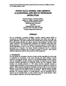
Automatic extraction of the knowledge embedded within the large volumes of data—that is, data mining—is a prevalent research theme. Unfortunately, the inherent structures and relations that are sought for may not be easily recognizable due to a complexity of high-dimensional data. This is particularly true when chemical and biologic problems are considered. Therefore, the need for advanced tools transforming high-dimensional data into a lower dimensionality space (dimensionality reduction) cannot be overestimated. This chapter describes a number of advanced dimensionality reduction techniques, both linear and nonlinear (Fig. 15.1). The following linear methods are described: principal component analysis (PCA) [1], linear discriminant analysis (LDA) [2], and factor analysis (FA) [3]. Among nonlinear methods are kernel PCA (KPCA) [4], diffusion maps (DMs) [5], multilayer autoencoders (MAs) [6], Laplacian eigenmaps [7], Hessian local linear embedding (HLLE) [8], local tangent space analysis (LTSA) [9], locally linear coordination (LLC) [10], multidimensional scaling (MDS) [11], local linear embedding (LLE) [12], and support vector machines (SVMs) [13]. Though this list includes the most popular in computational chemistry techniques, it is not exhaustive; some less important approaches (like, e.g., ICA [14]) are deliberately omitted. Also, because of the space limitations some nonlinear techniques (which may often be considered “flavors” of more general approaches) are not described. To only mention, they are principal curves [15], curvilinear component analysis (CCA) [16], generalized discriminant analysis (GDA) [17], kernel maps [18], maximum variance unfolding (MVU) [19], conformal eigenmaps (CEMs) [20], locality preserving projections (LPPs) [21], linear local tangent space

2

3

Dimensionality reduction

Linear techniques

Diffusion distance

PCA, LDA, FA LLTSA, LPP, linear SVM Distance preservation

Diffusion map

Metric distances

Geodesic distance IsoMap GNA

Re

52

c15.indd 424

SPE

Nonlinear techniques

Preserving global properties

Kernel-based

Global alignment of linear models

Preserving local properties

Neural network

Kernel-based CCA, MA, PCA, SVM, maps. Kohonen SOM GDA, MVU

LLC

Tangent space

Hessian LLE, LTSA

Reconstruction weights

Neighborhood graph Laplacian

LLE

Laplacian eigenmaps, CEM

PC, FastMap Sammon maps, MDS

Figure 15.1  A functional taxonomy of advanced dimensionality reduction techniques. GNA = ••; SOM = ••.

8/27/2009 4:21:55 PM

Dimensionality Reduction Basics

425

alignment (LLTSA) [22], FastMap [23], geodesic nullspace analysis (GNA) [24], and various methods based on the global alignment of linear models [25–27]. Finally, it should be noted that several advanced mapping techniques (selforganizing Kohonen maps [28], nonlinear Sammon mapping [29], IsoMap [30,31], and stochastic proximity embedding [SPE] [32]) are described in more detail; see Chapter 16 of this book.

15.2  Dimensionality Reduction Basics In silico pharmacology is an explosively growing area that uses various computational techniques for capturing, analyzing, and integrating the biologic and medical data from many diverse sources. The term in silico is an indicative of procedures performed by a computer (silicon-based chip) and is reminiscent of common biologic terms in vivo and in vitro. Naturally, in silico approach presumes massive data mining, that is, extraction of the knowledge embedded within chemical, pharmaceutical, and biologic databases. A particularly important aspect of data mining is finding an optimal data representation. Ultimately, we wish to be able to correctly recognize an inherent structure and intrinsic topology of data, which are dispersed irregularly within the high-dimension feature space, as well as to perceive relationships and associations among the studied objects. Data structures and relationships are often described with the use of some similarity measure calculated either directly or through the characteristic features (descriptors) of objects. Unfortunately, the very essence of similarity measure concept is intimately connected with a number of problems, when applied to high-dimensional data. First, the higher is the number of variables, the more probable is a possibility of intervariable correlations. While some computational algorithms are relatively insensitive to correlations, in general, redundant variables tend to bias the results of modeling. Moreover, if molecular descriptors are used directly for property prediction or object classification, overfitting can become a serious problem at the next stages of computational drug design. Second, a common difficulty presented by huge data sets is that the principal variables, which determine the behavior of a system, are either not directly observable or are obscured by redundancies. As a result, visualization and concise analysis may become nearly impossible. Moreover, there is always the possibility that some critical information buried deeply under a pile of redundancies remains unnoticed. Evidently, transforming raw high-dimensional data to the low-dimensional space of critical variables—dimensionality reduction—is a right tool to overcome the problems. For visualization applications, an ideal would be a mapping onto two-dimensional or three-dimensional surface.

c15.indd 425

8/27/2009 4:21:55 PM

Re

426

4

Re

c15.indd 426

Dimensionality Reduction Techniques

The principal aim of dimensionality reduction is to preserve all or critical neighborhood properties (data structure). This presumes that the data points located close to each other in high-dimensional input space should also appear neighbors in the constructed low-dimensional feature space. Technically, there exist many approaches to dimensionality reduction. The simplest ones are linear; they are based on the linear transformation of the original highdimensional space to target a low-dimensional one. Advanced nonlinear techniques use more complicated transforms. Evidently, nonlinear methods are more general and, in principle, applicable to a broader spectrum of tasks. This is why this chapter considers nonlinear techniques in more detail. However, it is worth mentioning that linear methods typically have mathematically strict formulation and, which is even more important, form a basis for sophisticated nonlinear techniques. The classical linear methods widely used in chemoinformatics are PCA [33] and MDS [34]. PCA attempts to transform a set of correlated data into a smaller basis of orthogonal variables, with minimal loss in overall data variance. MDS produces a low-dimensional embedding that preserves original distances (=dissimilarity) between objects. Although these methods work sufficiently well in case of linear or quasi-linear subspaces, they completely fail to detect and reproduce nonlinear structures, curved manifolds, and arbitrarily shaped clusters. In addition, these methods, as many of stochastic partitioning techniques, can be most effectively used for the detailed analysis of a relatively small set of structurally related molecules. They are not well suited for the analysis of disproportionately large, structurally heterogeneous data sets, which are common in modern combinatorial techniques and HTS systems. One additional problem of MDS is that it unfavorably scales quadratically with the number of input data points, which may require enormous com­ putational resources. Therefore, there exists a continuing interest to novel approaches. Some examples of such advanced methods are agglomerative hierarchical clustering based on two-dimensional structural similarity measurement, recursive partitioning, and self-organizing mapping, as well as generative topographic mapping and truncated Newton optimization strategy could be effectively used [35–37]. Thus, a variety of different computational approaches were recently intended to apply neural net paradigm toward a nonlinear mapping (NLM). The immense advantage of neural nets lies in their extraordinary ability to allocate the positions of new data points in the lowdimensional space producing significantly higher predictive accuracy. A number of scientific studies have successfully applied the basic self-organizing principles, especially self-organizing Kohonen methodology for visualization and analysis of the diversity of various chemical databases [38–40]. Sammon mapping [29] is another advanced technique targeted for dimensionality reduction, which is currently widely used in different scientific areas, including modern in silico pharmacology. Although the practical uses of this method is also weakened by the mentioned restriction relating to large data sets, it has

8/27/2009 4:21:55 PM

Dimensionality Reduction Basics

427

several distinct advantages as against to MDS. The basic principles of Sammon algorithm are discussed in more detail below. 15.2.1 Clustering Clustering is a common though simple computational technique widely used to partition a set of data points into groups (clusters) in such a manner that the objects in each group share the common characteristics, as expressed by some distance or similarity measure. In other words, the objects falling into the same cluster are similar to each other (internally homogeneous) and dissimilar to those in other clusters (externally heterogeneous). Based on the way in which the clusters are formed, all clustering techniques may be commonly divided into two broad categories: hierarchical, which partitions the data by successively applying the same process to clusters formed in previous iterations, or nonhierarchical (partitional), which determines the clusters in a single step [41]. Hierarchical algorithms are more popular as they require very little or no a priori knowledge. Hierarchical methods are divided in two minor classes: agglomerative (bottom-up) or divisive (top-down). In agglomerative analysis, clusters are formed by grouping samples into bigger and bigger clusters until all samples become members of a single cluster. Before the analysis, each sample forms its own, separate cluster. At the first stage, two samples are combined in the single cluster, at the second, the third sample is added to the growing cluster, and so on. Graphically, this process is illustrated by agglomerative dendrogram. Inversely, a divisive scheme starts with the whole set and successively splits it into smaller and smaller groups. There are two more important details: the way of measuring the distance between samples (metrics) and the way of measuring the distance between samples and cluster (linkage rule). The popular options are Euclidean, squared Euclidean, and Manhattan city-block metrics in combination with complete linkage, Ward’s linkage, and weighted/unweighted pair-group average linkage rules. Cluster analysis already found numerous applications in various fields including chemoinformatics. Because of its close ties with molecular similarity, clustering is often a tool of choice in the diversity analysis allowing one to reduce the complexity of a large data set to a manageable size [42,43]. Technically, clustering compounds comprises four principal steps. Initially, a rational set of molecular descriptors is selected (and, typically, scaled). Then pairwise distances between molecules are calculated and collected into similarity matrix. After that, cluster analysis technique is used to iteratively assign objects to different clusters. Finally, the clustering is validated, visually and/ or statistically. Many efforts to visualize the results of hierarchical and nonhierarchical clustering have been made based on graph drawing and tree layout algorithms.

c15.indd 427

8/27/2009 4:21:55 PM

Re

428

5

Re

c15.indd 428

Dimensionality Reduction Techniques

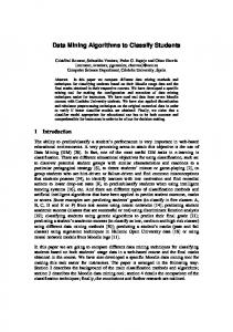
One popular option is the Jarvis–Patrick algorithm. This method begins by determining the k-nearest neighbors of each object within the collection. Members are placed in the same cluster if they have some predefined number of common nearest neighbors. The major advantage of this method lies in the speed of processing performance, but the main disadvantage is a regrettable tendency to generate either too many singletons or too few very large clusters depending on the stringency of the clustering criteria. Several key algorithms for graph construction, tree visualization, and navigation, including a section focused on hierarchical clusters, were comprehensively reviewed by Herman [44]; Strehl and Ghosh [45] inspected many computational algorithms for visualizing nonhierarchical clusters including similarity matrix plot. Still, a classical dendrogram remains the most popular cluster visualization method. This layout visually emphasizes both the neighbor relationship between data items in clusters (horizontal) and the number of levels in the cluster hierarchy (vertical). The basic limitation of radial space-filling and linear tree visualizations is the decreasing size and resolution of clusters with many nodes or deep down in the hierarchy. To overcome these challenges, Agrafiotis et al. [46] recently developed a new radial space-filling method targeted for visualizing cluster hierarchies. It is based on radial space-filling system and nonlinear distortion function, which transforms the distance of a vertex from the focal point of the lens. This technique has been applied (Fig. 15.2A,B) [47,48] for the visualization and analysis of chemical diversity of combinatorial libraries and of conformational space of small organic molecules [49]. In the first case, the radial clustergram represented a virtual combinatorial library of 2500 structures produced by combining 50 amines and 50 aldehydes via reductive amination. Each product was accurately described by 117 topological descriptors, which were normalized and decorrelated using PCA—to an orthogonal set of 10 latent variables accounting for 95% of the total variance in the input data. The obtained radial clustergram (Fig. 15.2) is color coded by the average molecular weight (A) and log P (B) (blue color corresponds to higher value); the two clusters designated as A and B are easily recognized. Note that color significantly changes at cluster boundaries, so one may reveal structurally related chemical families with distinct properties. While all of the tested structures share a common topology, which explains their proximity in diversity space, compounds located in cluster “A” contain several halogens as well as at least one bromine atom, which increases both their molecular weight and log P. There are no molecules in the first cluster with bromine atom, and none of them carry more than one light halogen (F or Cl). The second example (Fig. 15.2C,D) illustrates the application of radial clustergram for visualization of conformational space. The data set consisted of 100 random conformations of known HIV protease inhibitor, Amprenavir. Each pair of conformers was superimposed using a least-squares fitting procedure, and the resulting root mean square deviation (RMSD) was used as a

8/27/2009 4:21:55 PM

429

Dimensionality Reduction Basics

C

Cluster A

B

Cluster B

Cluster A

D 14

Cluster A

5

12

4.8

10

4.6

8 4.4

6

4.2

4

Radius gyration

A

4

2 2

4

6

8

10

12

14

Figure 15.2  Radial clustergrams of a combinatorial library containing 2500 compounds; color coding is by average molecular weight (A) and log P (B), radial clustergram (C), and SPE map (D) of conformational space around Amprenavir.

6

c15.indd 429

measure of the similarity between the two conformations. The radial clustergram color coded by the radius of gyration (a measure of the extendedness or compactness of the conformation) is shown in Figure 15.2C, while Figure 15.2D shows a nonlinear SPE map of the resulting conformations (see Section 15.4.1.7 for SPE description; the method embeds original data into a twodimensional space in such a way that the distances of points on the map are proportional to the RMSD distances of respective conformations). Among other modern algorithms related to clustering that should be mentioned are the maximin algorithm [50,51], stepwise elimination and cluster sampling [52], HookSpace method [53], minimum spanning trees [54], graph machines [55], singular value decomposition (SVD), and generalized SVD [56].

8/27/2009 4:21:56 PM

Re

430

Dimensionality Reduction Techniques

15.3 Linear Techniques For Dimensionality Reduction 15.3.1  PCA

7

8

Re

c15.indd 430

PCA, also known as Karhunen–Loeve transformation in signal processing, is a quite simple though powerful and popular linear statistical technique with a long success history [57–60]. It allows one to guess an actual number of independent variables and, simultaneously, to transform the data to reduced space. PCA is widely used to eliminate strong linear correlations within the input data space as well as to data normalization and decorrelation. By its essence, PCA constructs a low-dimensional representation of the input data, which describes as much of the variance of source data as possible [61]. Technically, it attempts to project a set of possibly correlated data into a space defined by a smaller set of orthogonal variables (principal components [PCs] or eigenvectors), which correspond to the maximum data variance. From a practical viewpoint, this method combines descriptors into a new, smaller set of noncorrelated (orthogonal) variables. In mathematical terms, PCs are directly computed by diagonalizing the variance covariance matrix, mij, a square symmetric matrix containing the variances of the variables in the diagonal elements and the covariances 1 1 N in the off-diagonal elements: mij = mji = ∑ ( xki − ξ i ) ( xkj − ξ j ); ξ i = ∑ xij , N N i =1 where ξi is the mean value of variable xi, and N is the number of observations in the input data set. Using this strategy, PCA attempts to find a linear mapping basis M that maximizes M T cov X − X M where cov X − X is the covariance matrix of zero mean data X (D-dimensional data matrix X). Such linear mapping can easily be formed by the d PCs derived from the covariance matrix mij. Principally, PCA attempts to maximize M T cov X − X M with respect to M, under the constraint |M| = 1. This constraint, in turn, can be consistently enforced by introducing a Lagrange multiplier λ. Hence, an unconstrained maximization of M T cov X − X M + λ (1 − M T M ) can be efficiently performed, then a stationary point of this expression can be regularly found assuming that cov X − X M = λM . Following this logic, PCA investigates the eigenproblem lying in cov X − X M = λM , which can be solved successfully for the d principal eigenvalue λ. The low-dimensional data representations encoded entirely by yi (the ith row of the D-dimensional data matrix Y) of the sample point xi (high-dimensional data points or the ith row of the D-dimensional data matrix X) can then be computed by mapping them onto the linear basis M, i.e., Y = ( X − X ) M. Considering that the eigenvectors of covariance matrix are the PCs while the eigenvalues are their respective variances, the number of PCs directly corresponds to the number of the original variables. In other words, PCA reduces the dimensionality of input data points by throwing off the insignificant PCs that contribute the least to the variance of the data set (i.e., PCs with the smallest eigenvalues) until the maximum variance approximates manually or machine predefined threshold, typically defined in the range of

8/27/2009 4:21:56 PM

Linear Techniques For Dimensionality Reduction

9

431

90–95% of the original input value. Finally, the input vectors are transformed linearly using the transposed matrix. At the output of PCA processing, the obtained low-dimensional coordinates of each sample in the transformed frame represent linear combinations of the original, cross-correlated variables. The immense advantage of PCA algorithm lies in the following statement: there are no assumptions toward the underlying probability distribution of the original variables, while the distinct disadvantage can be related meaningfully to a heightened sensibility to possible outliers, missing data, and poor correlations among input variables due to irregular distribution within the input space. Having due regard to all the advantages mentioned above, PCA is evidently not suitable for the study of complex chemoinformatics data characterized by a nonlinear structural topology. In this case, the modern advanced algorithms of dimensionality reduction should be used. For example, Das et al. [62] recently effectively applied a nonlinear dimensionality reduction technique based on the IsoMap algorithm [31] (see Section 15.4.1.6). 15.3.2 LDA LDA [2] is a linear statistical technique generally targeted for the separation of examined vector objects belonging to different categories. As PCA mainly operates on principle related to eigenvectors formation, LDA is generally based on a combination of the independent variables called discriminant function. The main idea of LDA lies in finding the maximal separation plan between external data points [2]. In contrast to the majority of dimensionality reduction algorithms described in this chapter, LDA can be regarded as a supervised technique. In essence, LDA finds a linear mapping image M that provides the maximum linear separation among the estimated classes in the low-dimensional representation of the input data. The major criteria that are primarily used to formulate a linear class separability in LDA are the withinclass scatter Zw and the between-class scatter Zb, which are correspondingly defined as Zw = ∑ pf cov X f − X f , Zb = cov X − X − Zw, where pf is the class prior f

of class label f, cov X f − X f is the covariance matrix of the zero-mean data point xi directly assigned to class f ∈ F (where F is the set of possible classes), while cov X − X is the covariance matrix of the zero-mean data assigned to X. In these terms, LDA attempts to optimize the critical ratio between Zw and Zb in the low-dimensional representation of the input data set, by finding a linear mapping image M that maximizes the so-called Fisher criterion: MT Z M φ ( M ) = T b . The post maximization problem can be efficiently solved M Zw M by computing the d principal eigenvectors of Zw−1Zb under the following requirement: d  0, this xi is an SV x. After minimization, decision function is written as m



  f ( x ) = sgn  ∑ yi α i ⋅ x ⋅ xi + b .  i =1 

Note that only a limited subset of training points, namely SVs, do contribute to the expression. In linearly inseparable case, where no error-free classification can be achieved by hyperplane, there still exist two ways to proceed with SVM.

Re

c15.indd 440

8/27/2009 4:21:58 PM

Nonlinear Techniques for Dimensionality Reduction

441

The first one is to modify linear SVM formulation to allow misclassification. Mathematically, this is achieved by introducing classification-error (slack) variables ξi > 0 and minimizing the combined quantity

m 1 2 W + C ∑ ξi , 2 i =1

under the constraint defined as yi(Wxi + b) ≥ 1 − ξi, I = 1 … m. Here, the parameter C regulates a trade-off between minimization of training error and maximization of margin. Such approach is known as soft margin technique. Another way is nonlinear SVM, which achieved a great deal of attention in the last decade. The most popular current approach is “transferring” data points from the initial descriptor space to space of higher dimension, which is derived by adding new degrees of freedom through nonlinear transformations of initial dimensions. The hope is that nonlinear in original space problem may become linear in higher dimensions, so that linear solution technique becomes applicable. Importantly, direct transfer of the points from original to higherdimensionality space is even not necessary, as all the SVM mathematics deals with dot products of variables (xi, xj) rather than with variable values xi, xj itself. All which is necessary is to replace dot products (xi, xj) with their higherdimensionality analogues, functions K(xi, xj) expressed over original variable x. The suitable function K is called kernel, and the whole approach is known as the kernel trick. Decision function in this case is written as m



f ( x ) = sgn  ∑ yi α i ⋅ K ( x, xi ) + b  .  i =1  The most common kinds of kernels are



K ( xi , x j ) = ( xi , x j + 1) − polynomial, d

K ( xi , x j ) = exp ( −r xi − x j

2

) − RBF,

K ( xi , x j ) = sigmoid ( η ( xi x j ) + a) − two-layer perceptron. Finally, let us list the main SVM advantages [S15]: 1. We can build any complex classifier and the solution is guaranteed to be the global optimum (no danger of getting stuck at local minima). It is a consequence of quadratic programming approach and of the restriction of space of possible decisions. 2. There are few parameters to elucidate. Besides the main parameter C, only one additional parameter is needed to determine polynomial or RBF kernels, which typically (as can be judged from literature) demonstrate high classification power.

c15.indd 441

8/27/2009 4:21:58 PM

Re

442

Dimensionality Reduction Techniques

3. The final results are stable, reproducible, and largely independent of optimization algorithm. Absence of random constituent in SVM scheme guarantees that two users, which applied the same SVM model with the same parameters to the same data, will receive identical results (which is often not true with artificial neural networks).

16 17

18 19

In addition to topical application of SVM methodology toward various fields related to dimensionality reduction and pattern recognition, such as character recognition and text classification, SVM is currently widely used for the analysis of chemical data sets. For example, Pletnev et al. [86] tested the ability of SVM, in comparison with well-known neural network techniques, to predict drug-likeness and agrochemical-likeness for large compound collections. For both kinds of data, SVM outperforms various neural networks using the same set of descriptors. Also, SVM was used for estimating the activity of carbonic anhydrase II (CA II) enzyme inhibitors; it was found that the prediction quality of the SVM model is better than that reported earlier for conventional QSAR. Balakin et al. [35] effectively used a radial basis SVM classifier for the separation of compounds with different ADME profiles within the Sammon maps (Fig. 15.4). To sum up, SVMs represent a powerful machine learning technique for object classification and regression analysis, and they offer state-ofthe-art performance. However, the training of SVM is computationally expensive and relies on optimization. 15.4.2 Local Techniques Advanced mapping techniques described above are intended to embed global structure of input data into the space of low dimensionality. In contrast to this formulation, local nonlinear methods of dimensionality reduction are based

Re

Figure 15.4  Nonlinear Sammon models developed for compounds with different ADME properties supported by SVM classification: (A) human intestinal absorption, (B) plasma protein binding affinity, and (C) P-gp substrate efficacy. HIA = ••; 53 PPB = ••.

c15.indd 442

8/27/2009 4:21:59 PM

Nonlinear Techniques for Dimensionality Reduction

443

solely on preserving structure of small neighborhood of each data point. The key local techniques include LLE, Laplacian eigenmaps, HLLE, and LTSA. Of note, local techniques for dimensionality reduction can be freely viewed in the context of specific local kernel functions for KPCA. Therefore, these techniques can be cleverly redefined using the KPCA framework [87,88]. 15.4.2.1  LLE  LLE is a simple local technique for dimensionality reduction, which is generally similar to IsoMap algorithm in relying on the nearest neighborhood graph representation of input data points [12]. In contrast to IsoMap, LLE attempts to preserve solely the local structure of multivariate data. Therefore, the algorithm is much less sensitive to short-circuiting than IsoMap. Furthermore, the complete preservation of local properties often leads to successful embedding of nonconvex manifolds. In formal terms, LLE tries to modify the local properties of the manifold around the processed data sample xi by representing the data point as a linear combination wi (the so-called reconstruction weight coefficients) of its knearest neighbor xij. Hence, using the data point xi and a set of its nearest neighbors, LLE fits a hyperplane, making the bold assumption that the manifold is locally linear (the reconstruction weight wi of the data point xi is completely invariant to space rotation and translation, as well as rescaling). Due to the invariance, any linear mapping of the hyperplane into a lowdimensional space faithfully preserves the reconstruction weights within the space of lower dimensionality. In other words, if the local topology and geometry of the manifold are largely preserved in low-dimensional data representation, the reconstruction weight coefficient wi, which explicitly manipulates the data point xi and its adjacent array in high-dimensional data representation, also reconstructs the data point yi from its neighbors in lowdimensional space. The main idea of LLE is to find the optimal D-dimensional data representation F by adaptive minimization of the cost function: 2

k   φ ( F ) = ∑  yi − ∑ wij yij  . It can be clearly shown that φ(F) = (F − WF)2 =    i j =1

FT(I − W)T(I − W)F is the common function that should to be further minimized. In this conventional formulation, I is the n × n identity matrix. Hence, the target coordinates of the low-dimensional representations yi that minimize the cost function φ(F) can be easily found by computing the eigenvectors of (I − W)T(I − W) corresponding to the smallest d nonzero eigenvalues of the inproduct of (I − W) from the solution set. LLE has been successfully applied in various fields of data mining, including a super-resolution task [89] and sound source localization [90], as well as chemical data analysis [86]. Reportedly, LLE demonstrated poor performance in chemoinformatics. For example, this method has recently been reported to persistently fail in the visualization of even simple synthetic biomedical data sets [91]. It was also experimentally shown that in some cases, LLE performs

c15.indd 443

8/27/2009 4:21:59 PM

Re

444

Dimensionality Reduction Techniques

worse than IsoMap [92]. Probably, this may be attributed to the extreme sensitivity of LLE learning algorithm to “holes” in the manifolds [12].

20

15.4.2.2  HLLE  HLLE is an advanced variant of the basic LLE technique that minimizes the curvilinear structure of high-dimensional manifold by quasi-non-linear embedding it into a low-dimensional space, making a hypothetical assumption that the low-dimensional data representation is locally isometric [8]. The basic principle of HLLE lies in the eigenanalysis of a matrix Ω that describes the curviness of the manifold determined around the processed data points, which is directly measured by means of the local Hessian. The key aspect of the local Hessian sack constructed in a local tangent space at the data point is invariance to differences in positions of the data points processed. It can be straightforwardly shown that the target low-dimensional coordinates can be easily found by performing an eigenanalysis of the core matrix Ω. The algorithm starts with identifying the knearest neighbors for each data point xi based on Euclidean distance. Then, the local linearity of the manifold through the xi nearest neighborhood is conservatively assumed. Hence, a principal basis describing a local tangent space at the data point xi can be readily constructed using PCA performed across the k-nearest neighbor xij. In mathematical terms, a basis for the local tangent space for every data point xi can be routinely determined by computing the d principal eigenvectors M = {m1, m2, … , md} of the covariance matrix cov xij − xij . It should be particularly noted that the above formulation strongly requires the following rigid restriction: k ≥ d. Subsequently, an unbiased machine estimator for the Hessian sack of the manifold at point xi in local tangent space coordinates is explicitly computed. For the practical realization of this computational task, the matrix Zi is then meticulously formed. Containing (in the columns) all the cross products of M up to the dth order (including a column with ones), this matrix becomes orthonormalized after applying the Gram–Schmidt procedure. The expression of the tangent Hessian Hi can be further assayed by the transpose of the last 1 d ( d + 1) columns of the orthonormalized matrix Zi. Using Hessian estima2 tors in local tangent coordinates, the core matrix Ω can then be easily con structed basedon Hessian entries H im = ∑ ∑ (( H i ) jl × ( H i ) jm ). Consequently, i

j

the target matrix contains information related to the curviness of high-dimensional data manifold. Thus, the eigenanalysis of the matrix Ω is performed mainly in order to find the low-dimensional data representation that appropriately minimizes the curviness of the manifold, while the eigenvectors corresponding to the d smallest nonzero eigenvalues of matrix Ω are selected and, in turn, construct the feature matrix Y, which contains a low-dimensional representation of the input data space. 15.4.2.3  Laplacian Eigenmaps  Laplacian eigenmap algorithm [7] preserves local data structure by computing a low-dimensional representation of

Re

c15.indd 444

8/27/2009 4:21:59 PM

Nonlinear Techniques for Dimensionality Reduction

445

the data in which the distances between a data point and its k-nearest neighbors are minimized as far as possible. To describe a local structure, the method uses a simple rule: The distance in the low-dimensional data representation between the data point and the first nearest neighbor contributes more to the cost function than the distance to the second nearest neighbor. Thus, the minimization of the cost function that can be formally defined as the key eigenproblem is effortlessly achieved in the context of spectral graph theory. Initially, the algorithm constructs the neighborhood graph G in which every data point xi is directly connected to its k-nearest neighbors. Then, using the Gaussian kernel function, the weight of the edge can be easily computed for all the data points xi and xj constructing the graph G, thereby leading to a sparse adjacency matrix W. During the computation of the lowdimensional representation yi, the core function can be strictly defined as 2 φ (Y ) = ∑ ( yi − y j ) wij , where the large weight wij corresponds to small ij

distances between the processed data points xi and xj. Therefore, the potential difference between their low-dimensional representations yi and yj highly contributes to this cost function. As a consequence, nearby points in the highdimensional space are also brought closer together in the low-dimensional representation. In the context of the eigenproblem, the computation of the degree matrix M and the graph Laplacian L of the graph W jointly formulate the minimization task postulated before, so that the degree matrix M of W is a diagonal matrix, whose entries are the row sums of W (i.e., mij = ∑ wij ), whereas the j

graph Laplacian L can be easily computed using the following definition: L = M − W. Summarizing these basic postulates, the cost function can be 2 further redefined in φ (Y ) = ∑ ( yi − y j ) wij = 2Y T LY. Therefore, the minimiij

zation of the φ(Y) can then be performed equivalently by minimizing the YTLY. Finally, for the d smallest nonzero eigenvalues, the low-dimensional data representation Y can subsequently be found by solving the genera­ lized eigenvector problem defined as Lν = λMν. Summing up the aspects and advantages listed above, we can reasonably conclude that Laplacian eigenmaps represents at least not less powerful computational technique for lowdimensional data representation compared with LLE. It can be successfully applied in various fields of data mining, including chemoinformatics.

15.4.2.4  LTSA  LTSA, a technique that is quite similar to HLLE, attempts to screen local properties within the high-dimensional data manifold using the local tangent space of each data point [9]. The fundamental principle of LTSA lies in the following statement: [being artificially restricted by the key assumption of local linearity of the manifold] there exists a linear mapping from a high-dimensional data point to its local tangent space; also, there exists a linear

c15.indd 445

8/27/2009 4:21:59 PM

Re

446

21

Dimensionality Reduction Techniques

mapping from the corresponding low-dimensional data point to the same local tangent space [9]. Thus, LTSA attempts to align these linear mappings in such a way that they construct a local tangent space of the manifold from a lowdimensional representation. In other words, the algorithm simultaneously searches for the feature coordinates of low-dimensional data representations as well as for the linear mappings of low-dimensional data points to the local tangent space of high-dimensional data. Similar to HLLE, the algorithm starts with computing specific bases (partly resembling Hessian sacks) for the local tangent spaces at data point xi. This can be successfully achieved by applying PCA toward the k data point xij that is a neighbor of the data point xi results in a mapping (Mi) from the neighboring set of xi to the local tangent space Ωi. The most unique trait of this space lies in the existence of the linear mapping Li from the local tangent space coordinates xij to the low-dimensional representations yij. Using this property, LTSA performs the following minimi2 zation: min  ∑ Yi J k − Li Ωi , where Jk is the centering matrix of size k [67]. Yi , Li

i

It can be mathematically shown that the target solution of the posed minimi­ zation problem can be found readily using the eigenvectors of an align­ ment matrix B that correspond to the d smallest nonzero eigenvalues of B. For one turn, the components of the alignment matrix B can then be obtained as a result of iterative summation across all the matrices Vi start­ ing from the initial values of bij = 0, for ∀ij. It can also be shown that BN i N i = BN i N i + J k ( I − Vi ViT ) J k , where Ni is the selection matrix that contains the indices of the nearest neighbors around the data point xi. Finally, the low-dimensional representation Y can be readily obtained by computation of the eigenvectors of the symmetric matrix 21 ( B + BT ) that correspond to the d smallest nonzero eigenvectors. LTSA have been successfully applied to solving various data mining tasks occurring widely in the chemoinformatic field, such as the analysis of protein microarray data [93].

22

Re

c15.indd 446

15.4.2.5  Global Alignment of Linear Models  In contrast to the sections presented previously, where we have willingly discussed two major approaches to construction of a low-dimensional data representation by preserving the global or local properties of input data, the current section briefly describes key mapping techniques widely used for performing the global alignment of linear models, computing the corresponding number of linear models, and constructing a low-dimensional data representation by aligning the linear models obtained. Among a small number of methods targeted for the global alignment of linear models, LLC is a hugely promising technique broadly used for dimensionality reduction [10]. The bright idea of this method lies in computing the set of factor analyzers (see Section 15.4.3) by which the global alignment of the mixture of linear models can be subsequently achieved. The algorithm mainly proceeds in two principal steps: (1) computing the mixture of factor

8/27/2009 4:21:59 PM

References

447

analyzers for the input data set by means of an expectation maximization (EM) algorithm and (2) subsequent aligning of the constructed linear models in order to obtain a low-dimensional data representation using a variant of LLE. It should be especially noted that besides LLC, a similar technique called manifold charting has also been developed recently on the bias of this common principle [24]. Initially, LLC recruits a group of m factor analyzers using the EM algorithm [94]. Then, the obtained mixture outputs the local data representation yij and corresponding responsibility rij (where j ∈ {1, … , m}) for every input data point xi. In meticulous detail, the responsibility rij describes the connection between extent data point xi and the linear model j, so it trivially satisfies ∑ rij = 1. Using the set of estimated linear models and the corresponding i

responsibilities, responsibility-weighted data representations wij = rijyij can be readily computed and stored in an n × mD block matrix W. The global alignment of the linear models is then performed based on matrix W and matrix M defined by M = (I − F)T(I − F), where F is the matrix containing the reconstruction weight coefficients produced by LLE (see Section 15.4.2.1), and I denotes the n × n identity matrix. LLC analyzes a set of linear models by solving the generalized eigenproblem Aν = λBν for the d smallest nonzero eigenvalues. In this equation, A denotes the inproduct of MTW, whereas B denotes the inproduct of W. It can easily be shown that d eigenvector vi computed from the matrix L uniquely defines a linear mapping projection from the responsibility-weighted data representation W to the underlying lowdimensional data representation Y. Finally, the low-dimensional data representation can be obtained immediately by computing the following equation: Y = WL. References

23

24

c15.indd 447

1. Pearson K. On lines and planes of closest fit to systems of points in space. Philosophical Magazine 1901;2:559–572. 2. Fisher RA. The use of multiple measurements in taxonomic problems. Ann Eugen 1936;7:179–188. 3. Gorsuch RL. Common factor analysis versus component analysis: Some well and little known facts. Multivariate Behav Res 1990;25:33–39. 4. Mika S, Scholkopf D, Smola AJ, Muller K-R, Scholz M, Ratsch G. Kernel PCA and de-noising in feature spaces. In: Advances in Neural Information Processing Systems, edited by •• ••, pp. ••–••. Cambridge, MA: The MIT Press, 1999. 5. Nadler B, Lafon S, Coifman RR, Kevrekidis IG. Diffusion maps, spectral clustering and the reaction coordinates of dynamical systems. Appl Comput Harm Anal 2006;21:113–127. 6. Hinton GE, Salakhutdinov RR. Reducing the dimensionality of data with neural networks. Science 2006;313:504–507.

8/27/2009 4:21:59 PM

Re

448

25

26 27

28

29

30

Re

31

c15.indd 448

Dimensionality Reduction Techniques

7. Belkin M, Niyogi P. Laplacian eigenmaps and spectral techniques for embedding and clustering. In: Advances in Neural Information Processing Systems, edited by •• ••, Vol. 14, pp. 585–591. Cambridge, MA: The MIT Press, 2002. 8. Donoho DL, Grimes C. Hessian eigenmaps: New locally linear embedding techniques for high-dimensional data. Proc Natl Acad Sci USA 2005;102:7426–7431. 9. Zhang Z, Zha H. Principal manifolds and nonlinear dimensionality reduction via local tangent space alignment. SIAM J Sci Comput 2004;26:313–338. 10. Teh YW, Roweis ST. Automatic alignment of hidden representations. In: Advances in Neural Information Processing Systems, edited by •• ••, Vol. 15, pp. 841–848. Cambridge, MA: The MIT Press, 2002. 11. Cox T, Cox M. Multidimensional Scaling. London: Chapman & Hall, 1994. 12. Roweis ST, Saul LK. Nonlinear dimensionality reduction by locally linear embedding. Science 2000;290:2323–2326. 13. Vapnik V, Golowich S, Smola A. Support vector method for function approximation, regression estimation, and signal processing. Adv Neural Inf Process Syst 1996;9:281–287. 14. Bell AJ, Sejnowski TJ. An information maximization approach to blind separation and blind deconvolution. Neural Comput 1995;7:1129–1159. 15. Chang K-Y, Ghosh J. Principal curves for non-linear feature extraction and classification. In: Applications of Artificial Neural Networks in Image Processing III, edited by •• ••, pp. 120–129. Bellingham, WA: SPIE, 1998. 16. Demartines P, Herault J. Curvilinear component analysis: A self-organizing neural network for nonlinear mapping of data sets. IEEE Trans Neural Netw 1997;8: 148–154. 17. Baudat G, Anouar F. Generalized discriminant analysis using a kernel approach. Neural Comput 2000;12:2385–2404. 18. Suykens JAK. Data visualization and dimensionality reduction using kernel maps with a reference point. Internal Report 07–22; ESAT-SISTA, Leuven, Belgium, 2007. 19. Weinberger KQ, Packer BD, Saul LK. Nonlinear dimensionality reduction by semi-definite programming and kernel matrix factorization. Proceedings of the Tenth International Workshop on Artificial Intelligence and Statistics (AISTATS05), Barbados, West Indies, January 10, 2005. 20. Sha F, Saul LK. Analysis and extension of spectral methods for nonlinear dimensionality reduction. In: Proceedings of the 22nd International Conference on Machine Learning, Vol. 119, edited by •• ••, pp. 785–792. Bonn, Germany: ••, 2005. 21. He X, Niyogi P. Locality preserving projections. In: Advances in Neural Information Processing Systems, Vol. 16, edited by •• ••, p. 37. Cambridge, MA: The MIT Press, 2004. 22. Zhang T, Yang J, Zhao D, Ge X. Linear local tangent space alignment and application to face recognition. Neurocomputing 2007;70:1547–1533. 23. Faloutsos C, Lin K-I. FastMap: A fast algorithm for indexing, data-mining and visualization of traditional and multimedia datasets. In: Proceedings of 1995 ACM SIGMOD, Vol. 24, edited by •• ••, pp. 163–174. ••: SIGMOD RECORD, 1995.

8/27/2009 4:22:00 PM

References

449

24. Brand M. From subspaces to submanifolds. Proceedings of the 15th British Machine Vision Conference, London, 2004. 32

25. Brand M. Charting a manifold. In: Advances in Neural Information Processing Systems, edited by •• ••, Vol. 15, pp. 985–992. Cambridge, MA: The MIT Press, 2002.

33

26. Roweis ST, Saul L, Hinton G. Global coordination of local linear models. In: Advances in Neural Information Processing Systems, edited by •• ••, pp. ••–••. Cambridge, MA: The MIT Press, 2001. 27. Verbeek J. Learning nonlinear image manifolds by global alignment of local linear models. IEEE Trans Pattern Anal Mach Intell 2006;28:1236–1250. 28. Kohonen T. The self-organizing map. Proc IEEE 1990;78:1464–1480. 29. Sammon JW. A non-linear mapping for data structure analysis. IEEE Trans Comput 1969;C-18:401–409.

34

30. Tenenbaum JB. Mapping a manifold of perceptual observations. In: Advances in Neural Information Processing Systems, edited by •• ••, Vol. 10, pp. 682–688. Cambridge, MA: The MIT Press, 1998. 31. Tenenbaum JB, de Silva V, Langford JC. A global geometric framework for nonlinear dimensionality reduction. Science 2000;290:2319–2323. 32. Agrafiotis DK. Stochastic algorithms for maximizing molecular diversity. J Chem Inf Comput Sci 1997;37:841–851.

35

33. Hotelling H, Educ J. Analysis of a complex of statistical variables into principal components. J Educ Psychol 1993;24:417–441, 498–520. 34. Borg I, Groenen PJF. Modern Multidimensional Scaling: Theory and Applications. New York: Springer, 1997. 35. Balakin KV, Ivanenkov YA, Savchuk NP, Ivaschenko AA, Ekins S. Comprehensive computational assessment of ADME properties using mapping techniques. Curr Drug Discov Technol 2005;2:99–113. 36. Yamashita F, Itoh T, Hara H, Hashida M. Visualization of large-scale aqueous solubility data using a novel hierarchical data visualization technique. J Chem Inf Model 2006;46:1054–1059. 37. Engels MFM, Gibbs AC, Jaeger EP, Verbinnen D, Lobanov VS, Agrafiotis DK. A cluster-based strategy for assessing the overlap between large chemical libraries and its application to a recent acquisition. J Chem Inf Model 2006;46: 2651–2660. 38. Bernard P, Golbraikh A, Kireev D, Chrétien JR, Rozhkova N. Comparison of chemical databases: Analysis of molecular diversity with self organizing maps (SOM). Analusis 1998;26:333–341. 39. Kirew DB, Chrétien JR, Bernard P, Ros F. Application of Kohonen neural networks in classification of biologically active compounds. SAR QSAR Environ Res 1998;8:93–107. 40. Ros F, Audouze K, Pintore M, Chrétien JR. Hybrid systems for virtual screening: Interest of fuzzy clustering applied to olfaction. SAR QSAR Environ Res 2000; 11:281–300. 41. Jain AK, Murty MN, Flynn PJ. Data clustering: A review. ACM Computing Surveys 1999;31:264–323.

c15.indd 449

8/27/2009 4:22:00 PM

Re

450

36

37

38

39

Re

c15.indd 450

Dimensionality Reduction Techniques

42. Brown RD, Martin YC. Use of structure-activity data to compare structure-based clustering methods and descriptors for use in compound selection. J Chem Inf Comput Sci 1996;36:572–584. 43. Bocker A, Derksen S, Schmidt E, Teckentrup A, Schneider G. A hierarchical clustering approach for large compound libraries. J Chem Inf Model 2005;45: 807–815. 44. Herman I. Graph visualization and navigation in information visualization: A survey. IEEE Trans Vis Comput Graph 2000;6:24–43. 45. Strehl A, Ghosh J. Relationship-based clustering and visualization for highdimensional data mining. INFORMS J Comput 2003;15:208–230. 46. Agrafiotis DK, Bandyopadhyay D, Farnum M. Radial clustergrams: Visualizing the aggregate properties of hierarchical clusters. J Chem Inf Model 2007;47: 69–75. 47. Agrafiotis DK. Diversity of chemical libraries. In: The Encyclopedia of Computational Chemistry, edited by •• ••, Vol. 1, pp. 742–761. Chichester, U.K.: John Wiley & Sons, 1998. 48. Agrafiotis DK, Lobanov VS, Salemme FR. Combinatorial informatics in the postgenomics era. Nat Rev Drug Discov 2002;1:337–346. 49. Agrafiotis DK, Rassokhin DN, Lobanov VS. Multidimensional scaling and visualization of large molecular similarity tables. J Comput Chem 2001;22:488–500. 50. Lajiness MS. ••. In: QSAR: Rational Approaches to the Design of Bioactive Compounds, edited by •• ••, pp. 201–204. Amsterdam: Elsevier, 1991. 51. Hassan M, Bielawski JP, Hempel JC, Waldman M. Optimization and visualization of molecular diversity of combinatorial libraries. Mol Divers 1996;2:64–74. 52. Taylor R. Simulation analysis of experimental design strategies for screening random compounds as potential new drugs and agrochemicals. J Chem Inf Comput Sci 1995;35:59–67. 53. Boyd SM, Beverly M, Norskov L, Hubbard RE. Characterizing the geometrical diversity of functional groups in chemical databases. J Comput Aided Mol Des 1995;9:417–424. 54. Mount J, Ruppert J, Welch W, Jain A. ••. IBC 6th Annual Conference on Rational Drug Design, Coronado, CA, December 11–12, 1996. 55. Goulon A, Duprat A, Dreyfus G. Graph machines and their applications to computer-aided drug design: A new approach to learning from structured data. In: Lecture Notes in Computer Science, edited by •• ••, Vol. 4135, pp. 1–19. Berlin: Springer, 2006. 56. Nielsen TO, West RB, Linn SC, Alter O, Knowling MA, O’Connell JX, Zhu S, Fero M, Sherlock G, Pollack JR, Brown PO, Botstein D, van de Rijn M. Molecular characterisation of soft tissue tumours: A gene expression study. Lancet 2002;359: 1301–1307. 57. Cooley W, Lohnes P. Multivariate Data Analysis. New York: Wiley, 1971. 58. Jolliffe IT. Principal Component Analysis, 2nd edn. New York: Springer-Verlag, 2002. 59. Martin EJ, Blaney JM, Siani MA, Spellmeyer DC, Wong AK, Moos WH. Measuring diversity: Experimental design of combinatorial libraries for drug discovery. J Med Chem 1995;38:1431–1436.

8/27/2009 4:22:00 PM

References

451

60. Gibson S, McGuire R, Rees DC. Principal components describing biological activities and molecular diversity of heterocyclic aromatic ring fragments. J Med Chem 1996;39:4065–4072. 61. Hotelling H. Analysis of a complex of statistical variables into principal components. J Educ Psychol 1933;24:417–441. 62. Das PD, Moll M, Stamati H, Kavraki LE, Clementi C. Low-dimensional, freeenergy landscapes of protein-folding reactions by nonlinear dimensionality reduction. Proc Natl Acad Sci USA 2006;103:9885–9890. 63. Cummins DJ, Andrews CW, Bentley JA, Cory M. Molecular diversity in chemical databases: Comparison of medicinal chemistry knowledge bases and databases of commercially available compounds. J Chem Inf Comput Sci 1996;36:750–763. 64. Scholkopf B, Smola AJ, Muller K-R. Nonlinear component analysis as a kernel eigenvalue problem. Neural Comput 1998;10:1299–1319. 65. Shawe-Taylor J, Christianini N. Kernel Methods for Pattern Analysis. Cambridge, U.K.: Cambridge University Press, 2004. 66. Lima A, Zen H, Nankaku Y, Miyajima C, Tokuda K, Kitamura T. On the use of kernel PCA for feature extraction in speech recognition. IEICE Trans Inf Syst 2004;E87-D:2802–2811. 67. Hoffmann H. Kernel PCA for novelty detection. Pattern Recognit 2007;40:863– 874. 68. Tomé AM, Teixeira AR, Lang EW, Martins da Silva A. Greedy kernel PCA applied to single-channel EEG recordings. IEEE Eng Med Biol Soc 2007; 40 ••:5441–5444. 41

69. Tipping ME. Sparse kernel principal component analysis. In: Advances in Neural Information Processing Systems, edited by •• ••, Vol. 13, pp. 633–639. Cambridge, MA: The MIT Press, 2000. 70. Lafon S, Lee AB. Diffusion maps and coarse-graining: A unified framework for dimensionality reduction, graph partitioning, and data set parameterization. IEEE Trans Pattern Anal Mach Intell 2006;28:1393–1403. 71. Kung SY, Diamantaras KI, Taur JS. Adaptive principal component EXtraction (APEX) and applications. IEEE Trans Signal Process 1994;42:1202–1217. 72. Hinton GE, Osindero S, The Y. A fast learning algorithm for deep belief nets. Neural Comput 2006;18:1527–1554. 73. Raymer ML, Punch WF, Goodman ED, Kuhn LA, Jain AK. Dimensionality reduction using genetic algorithms. IEEE Trans Evol Comput 2000;4:164–171. 74. Johnson MA, Maggiora GM. Concepts and Applications of Molecular Similarity. New York: Wiley, 1990. 75. Torgeson WS. Multidimensional scaling: I. Theory and method. Psychometrika 1952;17:401–419. 76. Kruskal JB. Non-metric multidimensional scaling: A numerical method. Phychometrika 1964;29:115–129. 77. Tagaris GA, Richter W, Kim SG, Pellizzer G, Andersen P, Ugurbil K, Georgopoulos AP. Functional magnetic resonance imaging of mental rotation and memory scanning: A multidimensional scaling analysis of brain activation patterns. Brain Res 1998;26:106–12.

c15.indd 451

8/27/2009 4:22:00 PM

Re

452

42

43

44

45

46

47

48

49

Re

c15.indd 452

Dimensionality Reduction Techniques

78. Venkatarajan MS, Braun W. New quantitative descriptors of amino acids based on multidimensional scaling of a large number of physicalchemical properties. J Mol Model 2004;7:445–453. 79. Hinton GE, Roweis ST. Stochastic neighbor embedding. In: Advances in Neural Information Processing Systems, edited by •• ••, Vol. 15, pp. 833–840. Cambridge, MA: The MIT Press, 2002. 80. Shepard RN, Carroll JD. Parametric representation of nonlinear data structures. In: International Symposium on Multivariate Analysis, edited by •• ••, pp. 561–592. New York: Academic Press, 1965. 81. Martinetz T, Schulten K. Topology representing networks. Neural Netw 1994;7: 507–522. 82. Agrafiotis DK, Lobanov VS. Nonlinear mapping networks. J Chem Info Comput Sci 2000;40:1356–1362. 83. Vapnik V. ••. [Estimation of Dependences Based on Empirical Data]. New York: Springer-Verlag, 1982. 84. Vapnik V. The Nature of Statistical Learning Theory. New York: Springer-Verlag, 1995. 85. Zernov VV, Balakin KV, Ivaschenko AA, Savchuk NP, Pletnev IV. Drug dis­ covery using support vector machines. The case studies of drug-likeness, agrochemical-likeness, and enzyme inhibition predictions. J Chem Inf Comput Sci 2003;43:2048–2056. 86. L’Heureux PJ, Carreau J, Bengio Y, Delalleau O, Yue SY. Locally linear embedding for dimensionality reduction in QSAR. J Comput Aided Mol Des 2004;18: 475–482. 87. Bengio Y, Delalleau O, Le Roux N, Paiement J-F, Vincent P, Ouimet M. Learning eigenfunctions links spectral embedding and kernel PCA. Neural Comput 2004;16:2197–2219. 88. Ham J, Lee D, Mika S, Scholkopf B. A kernel view of the dimensionality reduction of manifolds. Technical Report TR-110; Max Planck Institute for Biological Cybernetics, ••, Germany, 2003. 89. Chang H, Yeung D-Y, Xiong Y. Super-resolution through neighbor embedding. In: IEEE Computer Society Conference on Computer Vision and Pattern Recognition, edited by •• ••, pp. 275–282. ••: ••, 2004. 90. Duraiswami R, Raykar VC. The manifolds of spatial hearing. In: Proceedings of International Conference on Acoustics, Speech and Signal Processing, Vol. 3, edited by •• ••, pp. 285–288. ••: ••, 2005. 91. Lim IS, Ciechomski PH, Sarni S, Thalmann D. Planar arrangement of highdimensional biomedical data sets by Isomap coordinates. In: Proceedings of the 16th IEEE Symposium on Computer-Based Medical Systems, edited by •• ••, pp. 50–55. New York: Mount Sanai Medical School, 2003. 92. Jenkins OC, Mataric MJ. Deriving action and behavior primitives from human motion data. In: International Conference on Intelligent Robots and Systems, Vol. 3, edited by •• ••, pp. 2551–2556, ••: ••, 2002. 93. Teng L, Li H, Fu X, Chen W, Shen I-F. Dimension reduction of microarray data based on local tangent space alignment. In: Proceedings of the 4th IEEE

8/27/2009 4:22:00 PM

References

453

International Conference on Cognitive Informatics, edited by •• ••, pp. 154–159. ••: ••, 2005. 94. Ghahramani Z, Hinton GE. The EM algorithm for mixtures of factor analyzers. Technical Report CRG-TR-96-1; Department of Computer Science, University of Toronto, 1996. 95. Bohm H-J, Schneider G. Virtual Screening for Bioactive Molecules. New York: 51 John Wiley & Sons, 2000. 50

Re

c15.indd 453

8/27/2009 4:22:00 PM

Re

c15.indd 454

8/27/2009 4:22:00 PM

AUTHOR Query FORM Dear Author During the preparation of your manuscript for publication, the questions listed below have arisen. Please attend to these matters and return this form with your proof. Many thanks for your assistance. Query References

  Figure

Query

Remarks

Note that figures may have been relabelled for readability, please check.

1.

AUTHOR: Please note that References 1–86 and 91–95 have been renumbered as Reference 1, which was cited only in the abstract, has been deleted. Please confirm if the changes are correct.

2.

AUTHOR: Please define ICA.

3.

AUTHOR: Please note that the abbreviation PC for principal curves has been deleted so as not to confuse with the same abbreviation for principal component. Is this OK?

4.

AUTHOR: Please define HTS.

5.

AUTHOR: Please note that all figures will appear in black and white; hence, please indicate how to change those figures in the chapter wherein colors have been mentioned in the discussion in the text and in the figure legend.

6.

AUTHOR: Please note that “Section 15.4.1.7” has not been found in the chapter. Please change all instances to match the discussion.

7.

AUTHOR: Please check the equation mij = mji =

1 N

∑ (x

ki

− ξ i ) ( xkj − ξ j ); ξ i =

1 N

N

∑x . ij

i =1

Should “mji” be changed to “mij?” Re

BPD15

c15.indd 1

8/27/2009 4:22:00 PM

Re

c15.indd 2

8.

AUTHOR: “Following this logic, PCA investigates the eigenproblem lied in …” has been changed to “Following this logic, PCA investigates the eigenproblem lying in …” Is this correct?

9.

AUTHOR: Please note that “Section 15.4.1.6” has not been found in the chapter. Please change to match the discussion.

10.

AUTHOR: “… a measure of the error occurred between the pairwise distances …” has been changed to “… a measure of the error that occurred between the pairwise distances …” Is this correct?

11.

AUTHOR: Please define fMRI.

12.

AUTHOR: Please define SNE.

13.

AUTHOR: “… which in turn make possible the MDS to approximate…” has been changed to “… which in turn make it possible for the MDS to approximate…” Is this correct?

14.

AUTHOR: Please confirm if “… and then “learns” the underlying transform recruiting one or more multilayer perceptrons …” is correct.

15.

AUTHOR: Please confirm if instances of “[S3],” “[S14],” and “[S15]” are correct or if these should be changed to reference citations.

16.

AUTHOR: Should the citation Pletnev et al. be changed to L’Heureux et al. to match the list?

17.

AUTHOR: “… in comparison with well know neural network techniques …” has been changed to “… in comparison with well-known neural network techniques …” Is this correct?

18.

AUTHOR: Please define QSAR.

19.

AUTHOR: Please define ADME.

20.

AUTHOR: Please confirm if “…by quasi-nonlinear embedding it into a low-dimensional space…” is correct.

8/27/2009 4:22:00 PM

21.

AUTHOR: Please confirm if the sentence “This can be successfully achieved by applying PCA toward the k data point … from the neighboring set of xi to the local tangent space Ωi” is correct.

22.

AUTHOR: Please note that “Section 15.4.3” has not been found in the chapter. Please change to match the discussion.

23.

AUTHOR: Reference 4: Please provide the editor name(s) and page range.

24.

AUTHOR: Reference 5: Please confirm if the abbreviated journal title is correct.

25.

AUTHOR: Reference 7: Please provide the editor name(s).

26.

AUTHOR: Reference 9: Please confirm if the abbreviated journal title is correct.

27.

AUTHOR: Reference 10: Please provide the editor name(s).

28.

AUTHOR: Reference 15: Please provide the editor name(s).

29.

AUTHOR: Reference 20: This has been treated as a published proceeding. If this is correct, please provide the editor name(s) and publisher.

30.

AUTHOR: Reference 21: Please provide the editor name(s).

31.

AUTHOR: Reference 23: This has been treated as a published proceeding. If this is correct, please provide the editor name(s) and place of publication.

32.

AUTHOR: Reference 25: Please provide the editor name(s).

33.

AUTHOR: Reference 26: Please provide the editor name(s) and page range.

34.

AUTHOR: Reference 30: Please provide the editor name(s). Re

c15.indd 3

8/27/2009 4:22:00 PM

Re

c15.indd 4

35.

AUTHOR: Reference 33: Please confirm if References 33 and 61 are two different entries.

36.

AUTHOR: Reference 47: Please provide the editor name(s).

37.

AUTHOR: Reference 50: Please provide the article title and editor name(s).

38.

AUTHOR: Reference 54: If possible, please provide the article title.

39.

AUTHOR: Reference 55: Please provide the editor name(s).

40.

AUTHOR: Reference 68: Please provide the volume number.

41.

AUTHOR: Reference 69: Please provide the editor name(s).

42.

AUTHOR: Reference 79: Please provide the editor name(s).

43.

AUTHOR: Reference 80: Please provide the editor name(s).

44.

AUTHOR: Reference 83: If possible, please provide the original foreign title of this reference.

45.

AUTHOR: Reference 88: Please provide the city.

46.

AUTHOR: Reference 89: This has been treated as a published conference. If this is correct, please provide the editor name(s), place of publication, and publisher.

47.

AUTHOR: Reference 90: This has been treated as a published conference. If this is correct, please provide the editor name(s), place of publication, and publisher.

48.

AUTHOR: Reference 91: This has been treated as a published symposium. If this is correct, please provide the editor name(s).

49.

AUTHOR: Reference 92: This has been treated as a published conference. If this is correct, please provide the editor name(s), place of publication, and publisher.

8/27/2009 4:22:00 PM

50.

AUTHOR: Reference 93: This has been treated as a published conference. If this is correct, please provide the editor name(s), place of publication, and publisher.

51.

AUTHOR: Reference 95: This entry is originally Reference 1. As the abstract has been deleted, please indicate where this should be cited in the text or delete this reference.

52.

AUTHOR: Figure 15.1: Please define GNA and SOM.

53.

AUTHOR: Figure 15.4: Please define P-gp, HIA, and PPB.

Re

c15.indd 5

8/27/2009 4:22:00 PM