Partial Matching of 3D Shapes with Priority-Driven Search - cs.Princeton

Eurographics Symposium on Geometry Processing (2006) Konrad Polthier, Alla Sheffer (Editors)

Partial Matching of 3D Shapes with Priority-Driven Search T. Funkhouser and P. Shilane Princeton University, Princeton, NJ

Abstract Priority-driven search is an algorithm for retrieving similar shapes from a large database of 3D objects. Given a query object and a database of target objects, all represented by sets of local 3D shape features, the algorithm produces a ranked list of the c best target objects sorted by how well any subset of k features on the query match features on the target object. To achieve this goal, the system maintains a priority queue of potential sets of feature correspondences (partial matches) sorted by a cost function accounting for both feature dissimilarity and the geometric deformation. Only partial matches that can possibly lead to the best full match are popped off the queue, and thus the system is able to find a provably optimal match while investigating only a small subset of potential matches. New methods based on feature distinction, feature correspondences at multiple scales, and feature difference ranking further improve search time and retrieval performance. In experiments with the Princeton Shape Benchmark, the algorithm provides significantly better classification rates than previously tested shape matching methods while returning the best matches in a few seconds per query.

1. Introduction Large databases of 3D models are becoming available in a number of disciplines, including computer graphics, mechanical CAD, molecular biology, and medicine. As these databases grow, shape-based similarity search is emerging as a valuable tool for analysis and discovery. The goal of our work is to develop effective methods to retrieve from a database a ranked list of 3D models most similar in shape to a 3D model provided as a query. This problem is difficult because objects of the same type may not have exactly the same sets of parts (e.g., some chairs have arms and others don’t), and some parts that distinguish object types may be relatively small (e.g., the ears of a bunny). Shape representations that account only for global shape properties do not perform well at recognizing shapes in these situations. A common method for addressing this problem is to represent every object by a set of local shape features centered on points sampled from the object’s surface and then to compute a similarity metric for every pair of objects based on a cost function measuring the quality of matches in the optimally aligned set of feature correspondences (e.g., [BMP01, CJ96, JH99]). This approach is attractive because it is robust to shape variations within a class – as long as a few key shape features match, then the objects will c The Eurographics Association 2006.

match. The challenge is that the number of possible feature correspondence sets grows exponentially with the set size – naively checking all possible sets of k feature correspondences among n features on two objects takes O(nk ) operations. In practice, searching the space of potential feature correspondences for a single pair of surfaces can take several seconds or minutes, and using these methods to find the best matches in a large database is impractical. In this paper, we introduce a priority-driven algorithm for searching all objects in a database at once. The algorithm is given a query object and a database of target objects, all represented by sets of local shape features, and its goal is to produce a ranked list of the best target objects sorted by how well any subset of k features on the query match features on the target object. To achieve this goal, the system maintains a priority queue of potential sets of feature correspondences (partial matches) sorted by a cost function accounting for both feature dissimilarity and geometric deformation. Initially, all pairwise correspondences between the features of the query and features of target objects are loaded onto the priority queue. Then, at every step, the best partial match m is popped off the priority queue, new partial matches are created by extending m to include compatible feature correspondences, and those new partial matches are added to

T. Funkhouser & P. Shilane / Partial Matching of 3D Shapes with Priority-Driven Search

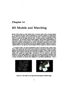
the priority queue. This process is iterated until the desired number of full matches with k feature correspondences have been popped off the priority queue. The advantage of this approach is that the algorithm provably finds the optimal set of matches over the entire database while investigating only a small subset of the potential matches. Like any priority-driven backtracking search (e.g., Dijkstra’s shortest path algorithm), the algorithm considers only the partial matches that can possibly lead to the lowest cost match (Figure 1). Although some poor partial matches are generated, they never rise to the top of the priority queue, and thus they incur little computational overhead. By using a single priority queue to store partial matches for all objects in the database at once, we achieve great speedups when retrieving only the top matches – if a small set of target objects match the query well, their feature correspondences will be discovered quickly and the details of other potential matches will be left unexplored. This approach largely avoids the combinatorial explosion of searching for multifeature matches in dissimilar objects. C4

Query A4

A1

Feature Matches ___________ Cost of Match

(A1,B2) (A2,B3) (A3,B1) 0.03

(A1,B3) (A2,B2) 0.12

Targets

C3 C1

A2

Low Cost

C2

A3

(A1,B2) (A2,B1) (A3,B3) 0.18

B1

B2

(A3,C1) 95.3

Priority Queue

B3

(A4,B1) 120.6

(A2,C3) 161.5

High Cost

Figure 1: Priority driven search: a priority queue (bottom) stores potential matches of features (labeled dots) on a query to features of all target objects at once. Matches are extended only when they reach the top of the priority queue (the leftmost entry), and thus high cost feature correspondences sit deep in the priority queue and incur little computational expense. This paper makes several research contributions. In addition to the idea of priority-driven search, we explore ways of improving computational efficiency and retrieval performance of multi-feature matching algorithms: 1) we use ranks rather than L2 differences to measure feature similarity; 2) we use a measure of class distinction to select features; and, 3) we match features at multiple scales. Finally, we provide a working shape-based retrieval system and analyze its performance over a wide range of options and parameter settings. We find that our system provides significantly better retrieval performance than previous shape matching approaches on the Princeton Shape Benchmark [SMKF04] while using increased, but reasonable, processing and storage costs. The organization of the paper is as follows. The next section contains a summary of related work on matching of

3D surfaces. Section 3 contains an overview of the prioritydriven search algorithm followed by a detailed description for every algorithmic step. Section 4 compares the performance of the priority-driven search approach to other stateof-the-art shape matching methods and investigates how modifying several aspects of the algorithm impacts its performance. Finally, Section 5 provides a brief discussion of limitations and topics for future work. 2. Background and Related Work There has been a large amount of research on algorithms for shape-based retrieval of 3D surface models. In this section, we focus on the previous work most closely related to ours and refer the reader to survey articles for broad overviews of prior work in related areas [BKS∗ 05, IJL∗ 05, TV04]. The most common approach to shape-based retrieval of 3D objects is to represent every object by a single global shape descriptor representing its overall shape. Shape Histograms [AKKS99], the Light Field Descriptor [COTS03], and the Depth Buffer Descriptor [HKSV02] are a few examples. These descriptors can be searched efficiently, and thus they are suitable for queries into large databases of 3D shapes. However, retrieval precision is generally poor when objects within the same class have different overall shapes – e.g., due to articulated motions, missing parts, or extra parts. Recently, several researchers have investigated approaches to partial shape matching based on feature correspondences (e.g., [BMP01, CJ96, GCO06, JH99, NDK05]). The general strategy is to compute multiple local shape descriptors (shape features) for every object, each representing the shape for a region centered at a point on the surface of the object. Then, the similarity of any pair of objects is determined by a cost function determined by the optimal set of feature correspondences at the optimal relative transformation, where the optimal match minimizes the differences between corresponding shape features and the geometric distortion implied by the feature correspondences. This approach has been used for recognizing objects in 2D images [BMP01, BBM05], recognizing range scans [JH99], registering medical images [AFP00], aligning point sets [CR00], aligning 3D range scans [GMGP05, LG05], and matching 3D surfaces [NDK05, SMS∗ 04]. The challenge is to find an optimal set of feature correspondences efficiently. One approach is to consider an association graph containing a node for every possible feature correspondence and an edge for every compatible pair of correspondences [BB76]. If each node is weighted by the dissimilarity of its associated features and each edge is weighted by the cost of the geometric deformation implied by its associated pair of correspondences, then finding the optimal set of k feature correspondences reduces to finding a minimum weight k-clique in the association graph. Researchers have approached this problem with algorithms c The Eurographics Association 2006.

T. Funkhouser & P. Shilane / Partial Matching of 3D Shapes with Priority-Driven Search

based on branch-and-bound [GMGP05], integer quadratic programming [BBM05], etc. However, previous work in this area has been aimed at pairwise alignment of objects, and current solution methods are generally too slow for search of large databases. Another approach is based on the RANSAC algorithm [FB81, SMS∗ 04]. Sets of k feature correspondences are generated, where k is large enough to determine an aligning transformation, and the remaining features are used to score how well the objects match after the implied alignment. For example, [JH99] finds small sets of compatible feature correspondences, computes the alignment providing a least-squared best fit of corresponding features, and then “verifies” the alignment with an iterative closest point algorithm [BM92]. [SMS∗ 04] proposed a “Batch RANSAC” version of this algorithm that considers matches to all target objects in a database all at once, generating candidate matches preferentially for the target objects with features compatible with ones in the query. However, their evaluation focused on recognition of vehicles from a small set of range scans, and studies have not been done to show how well it works for large databases of surface models. Several researchers have considered methods for accelerating database searches using discrete approximations. For example, geometric hashing [LW88] uses a grid-based hash table to store every feature of every target object in n choose k hash cells. For every query, k features are used to determine a mapping into the hash, and then other features vote for object transformations wherever there are hash collisions. This approach is quite popular in computer vision, molecular biology, and partial surface matching (e.g., [GCO06]). However, it requires a lot of memory to store hash tables and produces approximate matches, since it discretizes both the set of possible transformations (it only considers transformations induced by combinations of features) and Euclidean space (features match only if they fall in the same grid cell). Alternatively, “bag of words” approaches can be used to discretize feature space. For example, [MBM01] clusters features into “shapemes,” builds a histogram of shapemes for every object, and then approximates the similarity of two objects by the similarity of their histograms, and [GD05] extends this approach to consider pyramids of clusters. However, these methods make little or no use of the geometric arrangements of features, and thus they do not provide as distinguishing matches as possible. Our approach is to use priority-driven search to find the objects in a database that have sets of local feature correspondences minimizing a continuous cost function. The key idea is to use a priority queue to focus a backtracking search on sets of feature correspondences with lowest matching cost among all objects in the database all at once. This approach provides a significant efficiency improvement over more expensive algorithms that compute pairwise matches between the query and all objects in the database indepenc The Eurographics Association 2006.

dently (e.g., [BBM05]) – i.e., it avoids computing the optimal set of correspondences for the target objects that do not appear at the top of the retrieval list. It can also provide an accuracy improvement over discrete or greedy approximate algorithms, since it guarantees optimal matches with respect to a continuous cost function. 3. System Execution Execution of our system proceeds in two phases: a preprocessing phase and a query phase. During the preprocessing phase, we build a multi-feature representation of every object in the database. First, we generate for each object a set of spherical regions covering its surface at different scales. Second, for every region, we compute a descriptor of the shape within that region. Third, we compute differences between all pairs of descriptors at the same scale and associate with every descriptor a mapping from rank to difference. Finally, we select a subset of features to represent each object based on how distinctive they are of their object class. The result of this preprocessing is a set of “shape features” (or “features,” for short) for every object, each with an associated position (p), normal (~n), radius (r), and shape descriptor (a feature vector of numbers representing a local region of shape), and a description of how discriminating its shape descriptor is with respect to others in the database. For every query, our matching procedure proceeds as shown in Figure 2. The inputs are: 1) a query object, query, 2) a database of target objects, db, each represented by a set of shape features, 3) a cost function, cost, measuring the quality of a proposed set of feature correspondences, 4) a constant, k, indicating the number of feature correspondences that should be found for a complete match, and 5) a constant, c, indicating the number of objects for which to retrieve optimal matches. The output is a list of the best matching target objects, M, along with a description of the feature correspondences and cost for each one. Initially, a priority queue, Q, is created to store partial matches, and an array, M, is created to store the best match to every target object. Then, all pairwise correspondences between the features of the query and features of the target objects are created, stored in lists associated with the target objects, and loaded onto the priority queue. The priority queue then holds all possible matches of size 1. Then, until c complete matches have been found, the best partial match, m, is popped off the priority queue. If it is a complete match (i.e., the number of feature correspondences satisfies k), then the search of that target object is complete, and the priority queue is cleared of partial matches to that object. Otherwise, for every feature correspondence between the query and the target of m, the match is extended by one feature correspondence to form a new match, m0 . The best match for every target object is retained in an array, M, when it is added to

T. Funkhouser & P. Shilane / Partial Matching of 3D Shapes with Priority-Driven Search PriorityDrivenSearch(Object query, Database db, Function cost, int k, int c) # Create correspondences foreach Object target in db foreach Feature q in query foreach Feature t in target p = CreatePairwiseCorrespondence(q, t, cost) if (IsPlausible(p)) AddToPriorityQueue(Q, p) AddToList(C[target], p) if (cost(p) < cost(M[target])) M[target] = p # Expand matches until find complete ones complete_match_count = 0 while (complete_match_count < c) # Pop match off priority queue m = PopBestMatch(Q) target = GetTargetObject(m) # Check for complete match if (IsMatchComplete(m, k)) RemoveMatchesFromPriorityQueue(Q, target) complete_match_count++ continue; # Extend match foreach PairwiseCorrespondence p in C[target] m’ = ExtendMatch(m, p, cost) if (IsPlausible(m’)) AddToPriorityQueue(Q, m’) if (cost(m’) < cost(M[target])) M[target] = m’ # Return result return M

Figure 2: Pseudo-code for priority-driven search. the priority queue. This process is iterated until at least c full matches with k feature correspondences have been popped off the priority queue for c distinct target objects, and the array of the best matches to every target object, M, is returned as the result. The computational savings of this procedure come from two sources. First, matches are considered from best to worst, and thus, poor pairwise correspondences are never considered for extension and add little to the execution time of the algorithm. Second, after complete matches for at least c target objects have been added to the priority queue, it is possible to determine an upper-bound on the cost of matches that can plausibly lead to one of the best matches. If the score computed for an extended match, m0 , is higher than that upper bound, then there is no reason to add it to the queue, and it can be ignored. Similarly, if a match, m, is popped off the queue, then it is provably the best remaining match – i.e., no future match can be considered with a lower cost. Thus, the algorithm can terminate early (immediately after c best matches have been popped off the priority queue) while still guaranteeing an optimal solution.

Of course, there are many design decisions that impact the efficacy of this search procedure, including how regions are constructed, how shape descriptors are computed, what cost function is used, how implausible matches are culled, and so on. The following subsections describe our design decisions in detail, and Section 4 provides the results of experiments aimed at evaluating the impact of each one on search speed and retrieval performance. 3.1. Constructing Regions The first step of the process is to define a set of local regions covering the surface of every object. In theory, the regions could be volumetric or surface patches; they could be disjoint or overlap; and, they could be defined at any scale. In our system, we construct overlapping regions defined by spherical volumes centered on points sampled from the surface of an object [KPNK03, NDK05]. We have experimented with two different point sampling methods, one that selects points randomly with uniform distribution with respect to surface area, and another that selects points at vertices of the mesh with probability equal to the surface area of the vertices’ adjacent faces. However, they do not give significantly different performance, and so we consider only random sampling with respect to surface area for the remainder of this paper. Of course, other sampling methods that sample according to curvature, saliency, or other surface properties would be possible as well. We have experimented with regions at four different scales. The smallest scale has radius 0.25 times the radius of the entire object and the other scales are 0.5, 1.0, and 2.0 times, respectively. These scales are chosen because the smallest scale is approximately the size of most “distinguishing features of an object” and the largest scale is just big enough to cover the entire object for spheres centered at the most extreme positions on the surface (Figure 3). 0.25

0.5

1.0

2.0

Figure 3: Shape regions at four different scales. 3.2. Computing Shape Descriptors The second step of the process is to generate and store a representation of the shape for each spherical region (a shape descriptor). There will be many such regions for every surface, so the shape descriptors must be quick to compute, concise to store, and fast to compare, in addition to being as discriminating as possible. There are many shape descriptors that meet some or all of these criteria (see surveys in [BKS∗ 05, IJL∗ 05, TV04]). Examples include shape contexts [BMP01, MBM01, FHK∗ 04], c The Eurographics Association 2006.

T. Funkhouser & P. Shilane / Partial Matching of 3D Shapes with Priority-Driven Search

spin images [JH99, SMS∗ 04], harmonic shape descriptors [FHK∗ 04, NDK05], curvature profiles [CJ96, GCO06], and volume integrals [GMGP05]. In our system, we have experimented with three different shape descriptors based on spherical harmonics. All three decompose a sphere into concentric shells of different radii and then describe the distributions of shape within those shells using properties of spherical harmonics. The first (“SD”) simply stores the amplitude of all shape within each shell (the zero-th order component of spherical harmonics) – it is a one-dimensional descriptor equivalent to the “Shells” shape histogram of [AKKS99]. The second (“HSD”) stores the amplitude of spherical harmonic coefficients within each frequency – it is equivalent to the Harmonic Shape Descriptor of [FMK∗ 03,KFR03]. The last (“FSD”) descriptor stores the amplitude of every spherical harmonic coefficient separately – it is similar to the Harmonic Shape Contexts of [FHK∗ 04]. In all of our experiments, we utilize 32 spherical shells and 16 harmonic frequencies for each descriptor. We chose these shape representations for several reasons. First, they are well-known descriptors that have been shown to provide good performance in previous studies [FHK∗ 04, SMKF04]. Second, they are reasonably robust, concise, and fast to search. Finally, they provide a nested continuum with which to investigate the trade-offs between verbosity and discrimination – SD is very concise (32 values), but not that discriminating; HSD is more verbose (512 values) and more discriminating; and FSD is the most verbose (4352 values) and the most discriminating. The three descriptors are related in that each of the more concise descriptors is simply a subset or aggregation of terms in the more verbose ones (e.g., the SD descriptor stores the amplitude of only the zero-th order spherical harmonic frequencies). Thus, the L2 difference of each descriptor provides a lower bound on the L2 difference between the more verbose ones, which enables progressive refinement of descriptor differences, as proposed in Section 5. Our method for computing the descriptors for all regions of a single surface starts by computing a 3D grid containing the Euclidian Distance Transform of the surface. The grid resolution is chosen to match the finest sampling rate required by the HSD for regions at the smallest scale; the triangles of the surface are rasterized into the grid; and the squared distance transform is computed and stored. Then, for every spherical region centered on a point sampled from the surface, a spherical grid is constructed by aligning a sphere with the normal to the surface; a Gaussian function of the distance transform (GEDT) [KFR03] is sampled at regular intervals of radius and polar angles; the Spharmonickit software is used to compute the spherical harmonic decomposition for each radius; the amplitudes of the harmonic coefficients (or frequencies, depending on the type of shape descriptor) are computed; the shape descriptors are compressed using principal component analysis (PCA); and, the dimenc The Eurographics Association 2006.

sions associated with the top C eigenvalues (C ∼ 10%) are stored as a shape descriptor. For each 3D object, computing the three types of shape descriptors centered at 128 points for 4 scales (0.25, 0.5, 1.0, and 2.0) takes approximately four minutes overall and generates around 1MB of data per object. One minute is spent rasterizing the triangles and computing the squared distance transform at resolution sufficient for the smallest scale descriptors, almost two minutes are spent computing the spherical grids, and a few seconds are spent decomposing the grids into spherical harmonics for each object. Compression amortizes to approximately one minute per object for SFDs and approximately 1 second per object for SHDs. 3.3. Selecting Distinctive Features The third step of our process is to characterize the differences between shape descriptors and to select a subset of the shape features to be used for matching for each target object. Our goal is to augment the features with information about how discriminating they are and to select a subset of the most distinctive features in order to improve processing speed and retrieval precision. Selecting a subset of local shape descriptors is a well known technique for speeding up retrieval, and several researchers have proposed different methods for this task, The simplest technique is to select features randomly [JH99, FHK∗ 04, MBM01]. Other methods have considered selecting features based on surface curvature [YF02], saliency [GCO06], likelihood within the same shape [GMGP05, JH99], persistence across scales [GMGP05], number of matches to another shape [SMS∗ 04], likelihood within the database [SF06], and distinction of its object’s class [SF06]. In our system, we follow the ideas of [SF06]. For every feature, we compute the L2 difference of its shape descriptor to the best match of every other object in the database, sort the differences from best to worst, and save them in a rank-to-difference mapping (RTD). To save space, we store an approximation to the RTD containing log(N) values by sampling distances at exponentially larger ranks. We then use the RTD to estimate the distinction of every shape feature. Distinctive features are ones that are both similar to features in few other objects (ones in the same class) and different from the rest (objects in other classes). When given a classification for the target objects, we quantify this notion by using a measure of retrieval performance as our model for feature distinction [SF06]. Once the distinction of every feature has been computed, we employ a greedy algorithm to select a small set of features to represent every target object during the query phase (Figure 4). The selection algorithm iteratively chooses the feature with highest DCG whose position is not closer than a Euclidean distance threshold, minlength, to the position of

T. Funkhouser & P. Shilane / Partial Matching of 3D Shapes with Priority-Driven Search

any previously selected feature. This process avoids selecting features nearby each other on the mesh and provides an easy way to vary the subset size by adjusting the distance threshold.

(a) All Features

(b) Feature Distinction

(c) Selected Features

Figure 4: Feature selection: (a) positions sampled randomly on surface, (b) computed DCG values used to represent feature distinction (red is highest, blue is lowest), and (c) features selected to represent object during matching. The net result of this process is a small set of features for every target object, each with an associated position (p), normal (~n), radius (r), a set of shape descriptors (SD, HSD, and FSD), a rank-to-difference-mapping (RT D), and a retrieval performance score (DCG). In our implementation, computing the RTD and the distinction for each feature takes a little less than 1 second, and selecting the most distinctive features takes less than a second for each object. The storage required for the resulting data required at query time is approximately 100KB per object. 3.4. Creating Pairwise Feature Correspondences When given a query object to match to a database of target objects, the first step is to compute the cost of pairwise correspondences between features of the query to features of the target. The key to this step is to develop a cost function that provides low values only when two features are compatible and gradually penalizes pairs that are less similar. The simplest and most common approach is to use the L2 difference between their associated shape descriptors. This approach forms the basis for our implementation, but we augment it in three ways. First, given features F1 and F2 , we compute the L2 difference, D, between their shape descriptors. Then, we use the rank-to-difference mappings (RTD) of each feature to convert D into a rank (i.e., where that distance falls in the ranked list associated with each feature). The new difference measure (Crank ) is the sum of the ranks computed for F1 with respect to the RTD of F2 , and vice versa: Crank = Rank(RT D1 , D) + Rank(RT D2 , D) This feature rank cost (which we believe is novel) avoids the problem that very common features (e.g., flat planar regions) can provide indistinguishing matches (false positives) when L2 differences are small. Our approach considers not the absolute difference between two features, but rather their

difference relative to the best matching features of other objects in the database. Thus, a pair of features will only be considered similar if both rank highly in the retrieval list of the other. Second, we augment the cost function with geometric terms. For part-in-whole object matching, we can take advantage of the fact that features are more likely to be in correspondence if they appear at the same relative position and orientation with respect to the rest of their objects. Thus, for each feature, we compute the distance between its position and the center of mass of its object (R), scaled by the average of R for all features in the object (RAV G), and we add a distance term Cradius to the cost function accounting for the difference between these distances: Cradius = |

R1 R2 − | RAV G1 RAV G2

We also compute a normalized vector ~r from the object’s center of mass to the position of each feature and store the dot product of that vector with the surface normal (~n) associated with the feature. The absolute value of the dot product is taken to account for the possibility of backfacing surface normals. Then, the difference between dot products for any pair of features is used to form a normal consistency term to the cost function: Cnormal = ||~r1 · n~1 | − |~r2 · n~2 || Overall, the cost of a feature correspondence is a simple function of these three terms: γ

γ

γ

rank radius normal Ccorrespondence = αrankCrank +αradiusCradius +αnormal Cnormal

where the α coefficients and γ exponents are used to normalize and weight the terms with respect to each other. Of course, computing all potential pairwise feature correspondences between a query object and a database of targets is very costly. If the query has MQ features and each of N targets has MT selected features, then the total number of potential feature correspondences is N × MQ × MT . To accelerate this process, we utilize conservative thresholds on each of the three terms (maxrank, maxradius, maxnormal) to throw away obviously poor feature correspondences. The terms are computed and the thresholds are checked progressively in order of how expensive they are to compute (e.g., Crank is last), and thus there is great opportunity for trivial rejection of poor matches with little computation. Indexing and progressive refinement could further reduce the compute time as described in Section 5. 3.5. Searching for the Optimal Multi-Feature Match The second step of the query process is to search for the best multi-feature matches between the query object and the target objects. This is the main step of priority-driven search. c The Eurographics Association 2006.

Corres ponden ce

T. Funkhouser & P. Shilane / Partial Matching of 3D Shapes with Priority-Driven Search

Second, a surface orientation term is added to penalize matches with pairs of feature correspondences whose surface normals are inconsistent. This term penalizes both mismatches in the relative orientations of the two pairs of normals with respect to one other and mismatches in the orientations of the normals with respect to the chord between the features. If v~1 is the normalized vector between features 1a and 1b with normals n~1a and n~1b in object 1, and similar variables describe the relative orientations of features in object 2, then the orientation term of the cost function can be computed as follows:

Chord Point Sample

Corient =

Region

These terms are also weighted and raised to exponents to provide normalization when added to the overall scoring function computed for a match with k feature correspondences:

Shape Descriptor

Figure 5: A 3-feature match for two airplanes. Red points represent feature positions on the surface. For three features, red circles represent regions, gray histograms represent shape descriptors, orange lines represent feature correspondences, and black lines represent lengths between features of same object. Consistency of all shape descriptors, lengths, and angles is required for a good match.

A priority queue is used to store incomplete sets of feature matches during a backtracking search. Initially, all pairwise correspondences (computed as described in the previous subsection) are loaded onto the priority queue. Then, the best partial match, m, is repeatedly popped off the priority queue, and then extended matches are created for every compatible feature correspondence and loaded onto the priority queue. This process is iterated until at least c full matches with k feature correspondences have been popped off the priority queue for distinct target objects. As a partial match is extended to include one more feature correspondence, two extra terms are added to the cost function to account for geometric deformations implied by multiple pairwise feature correspondences (Figure 5). First, a chord length term Clength is added to penalize matches with inconsistent inter-feature lengths. Specifically, for every pair of feature correspondences in m, we compute the length of the chord between feature positions in the same object (L), scaled by the average of L over all features in the object (LAV G). Then, we compute the difference between these distances and normalize by the greater of the two to produce the length term of the cost function: Clength =

||n~1a · n~1b | − |n~2a · n~2b ||+ ||~ v1 · n~1a | − |~ v2 · n~2a ||+ ||~ v1 · n~1b | − |~ v2 · n~2b ||

L2 L1 | LAV G1 − LAV G2 |

L1 L2 max( LAV G1 , LAV G2 )

c The Eurographics Association 2006.

γ

γ

length orient Cchord = αlengthClength + αorient Corient

As in the previous section, we utilize conservative thresholds on Clength and Corient (maxlength and maxorientation) to throw away obviously poor feature correspondences. We also utilize a threshold on the minimum distance between features within the same object (minlength) in order to avoid matches comprised of features in close proximity to one another. The overall cost of a match is the sum of the terms representing differences in the k feature correspondences and the geometric differences between the k(k-1)/2 chords spanning pairs of features: Cmatch =

∑ Ccorrespondence (i) + ∑

i