extended as follows: (1) vortex tracking: the core lines are considered as connected ... at which the selected vortex is perturbed massively by another vortex, and .... Our definition of vortex core lines is similar to the definition of valley lines of the ...
ISFV13 - 13th International Symposium on Flow Visualization FLUVISU12 - 12th French Congress on Visualization in Fluid Mechanics July 1-4, 2008, Nice, France
PARTICLE-BASED VORTEX CORE LINE TRACKING TAKING INTO ACCOUNT VORTEX DYNAMICS Tobias Schafhitzel∗ , Kudret Baysal∗∗ , Ulrich Rist∗∗ , Daniel Weiskopf∗∗∗ , Thomas Ertl∗ ∗ Institute of Visualization and Interactive Systems, Universität Stuttgart ∗∗ Institute for Aerodynamics and Gasdynamics, Universität Stuttgart ∗∗∗ VISUS – Visualization Research Center, Universität Stuttgart KEYWORDS: Main subject(s): Flow Visualization, Vector Field Visualization Fluid: Incompressible Fluids Visualization method(s): Vortex Visualization, Segmentation, Vortex Tracking
ABSTRACT: The Investigation of the temporal behavior of coherent structures is a complex process. Particularly when vortices and their temporal change of strength or spatial extents are considered, a pure tracking of vortical structures is insufficient. The exploration of such properties makes it necessary to take into account the interaction between individual coherent structures, also called vortex dynamics. In this paper, we propose a framework which allows the tracking of segmented vortex structures taking into account vortex dynamics. Our framework is based upon an existing vortex core line detection and vortex segmentation implementation which is extended as follows: (1) vortex tracking: the core lines are considered as connected particles which are integrated along a given time-dependent vector field and tested against overlapping with the core lines of the following time step; (2) consideration of vortex dynamics: during the tracking process of a selected vortex, and for each time step, the vortex with the highest effect is computed; then the time step of the strongest perturbation t p is determined; (3) tracking of the perturbing vortices: starting at t p , the vortex structures with the highest effect are tracked along time to provide information about their temporal evolution; (4) visualization: vortical regions are represented by segmented λ2 isosurfaces which are highlighted using color coding and bounding boxes in the case they are tracked.
1
Introduction
The investigation of coherent structures in time-dependent flows is one of the most important applications in the field of fluid dynamics. Thereby, the name coherent structure can be ascribed to the spatial and temporal coherence which is required for the characterization of flow fields by the detection of organized structure motions. Particularly for the consideration of vortex dynamics, i.e., the interaction between different coherent structures, temporal coherence plays a crucial role. The capability of identifying vortex structures and their time-dependent development would allow an advanced study of kinematic properties, e.g., size, shape, energy, enstrophy, strength as well as the origin as dynamic properties of time-dependent flow fields [2]. The process of tracing several vortex structures along time is called vortex tracking, and its application reaches from basic research in fluid dynamics, ISFV13 / FLUVISU 12 - Nice / France - 2008
1
TOBIAS SCHAFHITZEL, KUDRET BAYSAL, ULRICH RIST, DANIEL WEISKOPF, THOMAS ERTL
e.g., for the comparison and validation of different simulation techniques, to the exploration of wind flows around vehicles in wind tunnels. Thereby one main concern of engineers is the backward-tracking of critical vortices, e.g., vortices which might influence the driving behavior negatively, to gain information about their temporal evolution. Here, the interaction between different vortex structures is not negligible, as particularly strong, spatially close vortices are able to influence the motion of their neighborhood. Consequently, though it is possible to classify a vortex as critical at time t p , the source of its criticality is not clear: either it could be the result of a negative effect of its neighbors, or the fact that a vortex generated at an unmeant location, or it could be a combination of both. The goal of this work is the detection of perturbation events on arbitrary temporarily tracked vortex structures. Starting with a segmented representation of the individual vortices, the vorticity inside each structure serves as input for the Biot-Savart equation, which computes the velocity induced from one vortex structure to another. In order to compute a global value which represents the influence of a vortex on the entire domain selected by the user, two different quantities are taken into account: kinetic energy and enstrophy. Both quantities are computed on the induced velocity field and its respective derivatives. Once the effect of each vortex on a selected structure is computed, the time t p of the highest perturbation is determined. This time serves as the starting point of a new tracking process which considers, in contrast to the previous vortex tracking, the critical vortex, i.e., the vortex with the highest effect as well as the selected vortex structure. This leads to a clear identification of critical perturbation events to an arbitrary vortex structure. The results of this computation are visualized within a graphical framework which provides the user full interaction in terms of selecting several vortex structures to explore their temporal behavior, and in particular, to gain information about their location and time of generation. In addition, the user is able to find out the time at which the selected vortex is perturbed massively by another vortex, and finally, to see where this critical vortex is coming from. 2
Previous Work
Pioneering work in analysis of vortex structures in order to investigate flow fields was done by Theodorsen [21]. The fundamental innovation of Theodorsen was the detection of socalled hairpin-like vortex structures and the importance of these structures for generation, conservation and spreading of turbulence. The detection of the hairpin-like vortex structures led to several approaches for turbulence models based on vortex structures [1], [2], [6], [16], [21]. However, the acceptance of these turbulence models was limited due to the fact that the vortex structures described by Theodorsen were not verifiable by experiments, caused by the limitations of experimental methods and the complexity of the structures. Only improvements in experimental methods [9] led to a verification of the hairpin-like vortex structures and to a broader acceptance of the turbulence models based on the work of Theodorsen. An enhancement of the single hairpin-like vortex structures was proposed by Adrian et al. [3]. In this approach, packages of hairpin-like vortices are considered, which are created by an autogeneration process. In previous work, the investigation of autogeneration is done by visualization of vortex structures alone (experiments or isosurface visualization of miscellaneous values in numerical results). The tools presented in this paper enable a more detailed investigation of the dynamical mechanisms of the structures. This is achieved by providing a representation of the temporal behavior of vortical structures taking into account their influence between each other, as well as tools for the exploration of vortices at a specific ISFV13 / FLUVISU 12 - Nice / France - 2008
2
PARTICLE-BASED VORTEX CORE LINE TRACKING TAKING INTO ACCOUNT VORTEX DYNAMICS
time. A vortex core line can be regarded as the geometrical and dynamical simplification of a three dimensional vortical region to a line. To the authors’ knowledge there exists no unique definition of a vortex core line; most of recent work bases on the assumption that the pressure is minimal along the vortex core line. Banks and Singer [5] proposed a predictor-corrector algorithm using the pressure and the vorticity for the identification of the core line. This method was extended by Stegmaier et al. [19] by replacing the pressure by the Galilean invariant λ2 quantity introduced by Jeong and Hussain [10]. Peikert reformulated most of the recent vortex core line detection methods using the parallel-vectors operator [15]. The parallel-vectors operator can be used to trace ridge and valley lines of local criteria like λ2 from local extremum points [17]. This idea can be extended to track core lines over time [20]. Recently, Weinkauf et al. [22] have extended this class of algorithms by proposing the coplanar-vectors operator, which is applied for the extraction of cores of swirling particle motion in transient flows. 3
Theoretical Basics on Vortices
In this section, a short introduction to the definition of vortical regions, the computation of vortex core lines and vortex dynamics is given. 3.1
λ2 Vortex Criterion
In recent research there exist various approaches for the identification of vortical regions [12, 7, 8, 10, 23]. One of the most effective methods is the λ2 method [10], which is based on the assumption of local pressure minima inside vortex structures. However, the computation of λ2 depends on the velocity gradient tensor, what makes the method Galilean invariant. For a more detailed description, we refer to the work of Jeong and Hussain [10]. The governing equation for the λ2 method is the Hessian of the the pressure p,i j : DSi j 1 − ν Si j,kk + Ωik Ωk j + Sik Sk j = − p,i j , Dt ρ
(1)
where ρ represents the density, S and Ω denote the symmetric and antisymmetric part of the velocity gradient tensor, and where the Einstein sum convention is applied. The first two terms on the left hand side are neglected in order to consider the inconsistency between the existence of a pressure minimum and the existence of a vortex. In the following, a brief description of the λ2 method is given. Let v(x) = (vx , vy , vz )T be a 3D vector field. Then, the velocity gradient tensor or Jacobian is defined as J = ∇v. By decomposition of this matrix into a symmetric and an antisymmetric part, the strain-rate tensor and the rotation tensor are obtained. The strain-rate tensor is defined by � 1 1 S = (J + J T ) with Si j = vi, j + v j,i , 2 2
(2)
� 1 1 Ω = (J − J T ) with Ωi j = vi, j − v j,i , 2 2
(3)
and the rotation tensor by
respectively. In order to compute λ2 , M = S2 + Ω2 is constructed. The tensor M is the corrected Hessian of pressure (see equation 1). Since M is real and symmetric, it has ISFV13 / FLUVISU 12 - Nice / France - 2008
3
TOBIAS SCHAFHITZEL, KUDRET BAYSAL, ULRICH RIST, DANIEL WEISKOPF, THOMAS ERTL
exactly three real eigenvalues, which can be sorted according to λ1 ≥ λ2 ≥ λ3 . The value for the λ2 vortex criterion is identical to the above eigenvalue λ2 . Vortex regions are defined as regions where λ2 < 0, i.e., vortex boundaries are given by isosurfaces of λ2 with isovalue 0. 3.2
Vortex Core Lines
The motivation of vortex core lines consists of the geometrical reduction of a vortical region to a line. Each vortical region detected by the λ2 criterion is supposed to have a rotation axis. This axis, called vortex core line, can be defined as the connection of local pressure minima, and as a connection of local λ2 minima [19],[14]. Our definition of vortex core lines is similar to the definition of valley lines of the λ2 scalar field. Therefore, each point on the valley line underlies a number of restrictions. Let us start with a 3D non-degenerate λ2 minimum, i.e., a point with a vanishing gradient ∇λ2 (x) = 0 and three positive eigenvalues of its Hessian H λ2 , which is a real symmetric matrix. The definition of valley lines relaxes these conditions, i.e., a point on the valley line is required to be a minimum perpendicular to its gradient, but in contrast to a 3D minimum, the λ2 value along the valley line should be allowed to vary. Let η0 ≥ η1 ≥ η2 be the eigenvalues and ε0 , ε1 , ε2 the respective eigenvectors of the Hessian at a point x. Then, λ2 (x) is a minimum on the plane spanned by ε0 and ε1 when η1 > 0. Peikert et al. [15] reformulated this problem using the parallel vectors operator with ∇λ2 ||∇(∇λ2 )∇λ2 , stating that the gradient of λ2 needs to be linearly dependent on the second derivative of λ2 along the gradient. However, this requires the computation of the second derivatives and its eigenvectors of λ2 , which might lead to inaccuracies due to noise. Both the predictor-corrector methods of Banks and Singer [5] and Stegmaier et al. [19] use the vorticity as an appropriate approximation of ε2 . In this paper, we follow the method of Stegmaier et al. to compute the vortex core lines. 3.3
Vortex Dynamics
The consideration of vortex dynamics enables a more detailed insight into the temporal behavior of coherent structures. In detail, vortex dynamics connect the evolution and interaction of coherent structures to their spatial extents. A simple method for the consideration of vortex dynamics consists of the analysis of dynamical values, e.g., kinetic energy or enstrophy: 1 Ekin = 2
Z
v (x,t)2 d 3 x,
(4)
1 = 2
Z
ω (x,t)2 d 3 x,
(5)
Erot
V
V
where V represents the 3D domain and ω denotes the vorticity. Thereby, the problem arises of a proper definition of the region of integration. In test cases with two vortex structures like collision of vortex rings [13], it is sufficient to integrate over the whole domain. In real flow fields containing hundreds of structures of interest, each of them needs a more specified definition of the integrated volume. Reasonable choices are the spatial extents of the vortical regions. Another technique supports the investigation of the interactions between vortex structures and other flow features, e.g., shear layers or other vortices. Particularly the interaction beISFV13 / FLUVISU 12 - Nice / France - 2008
4
PARTICLE-BASED VORTEX CORE LINE TRACKING TAKING INTO ACCOUNT VORTEX DYNAMICS
tween vortex structures is rather important, e.g., in 2D vortex merging [11] and in 3D collision of vortex rings [13]. The information obtained by identification, segmentation and tracking of vortex structures facilitates an intensified study of the interaction between several vortex structures. The fundamental equation for the analysis of vortex dynamics is the Biot-Savart, which computes the induced velocity field from vorticity: 1 vind (x,t) = 4π
Z
V
ω (x′ ,t) × (x − x′ ) 3 ′ d x. |x − x′ |3
(6)
In general, a velocity field can be represented as the sum of rotational and irrotational parts. The irrotational part is determined by the boundary conditions. The rotational velocity, denoted as vind in equation 6, is completely determined by the vorticity field. By computing the velocity induced by the vorticity field of a single vortex structure S1 , the influence of this structure on its environment is determined. Furthermore, by applying equation 4 or 5 to the induced velocity field, where the integration domain is restricted to a vortex structure S2 , the influence of S1 to S2 is determined. 4
Vortex Tracking taking into Account Vortex Dynamics
In this section, the tracking process is discussed, beginning with the detection of vortical regions, followed by the tracking of the vortex core lines and the consideration of vortex dynamics. The visualization of the results is discussed later in section 5. 4.1
Vortex Core Line Detection
Since our vortex core line detection method is based on the implementation of Stegmaier et al. [19], only a brief description is given. Based on the given velocity field, first the λ2 scalar field and the vorticity vector field are computed to use them as input for the skeleton growing algorithm. Starting at a 3D minimum of λ2 at position p0 , the skeleton grows in the direction of the vorticity vector and its opposite direction. After each integration step, a plane P perpendicular to the vorticity vector at the new position p′1 is computed to search the minimum λ2 value on it. This correction step determines the next position p1 on the vortex core line, which is supposed to be a minimum on P (see section 3.2). These two steps are repeated for each 3D minimum until one of the exit conditions, e.g., the exceed of the isovalue of the covering λ2 hull or a large deflection of the vorticity vectors, is fulfilled. The isosurface serves as spatial border for the growing vortex core line, and therefore, the λ2 isovalue should be chosen nearby 0. 4.2
Vortex Core Line Tracking
Once the vortex core lines and their respective λ2 isosurfaces are computed for each time step, we need to assign the structures at time t to their corresponding structures at time t + ∆t. This mapping process is called tracking. In this paper, vortex tracking is performed by particle tracing, where each particle is maintained by sampling the vortex core line. In the following this algorithm is discussed in more detail: let us consider a particle at an arbitrary position inside a vortex region, i.e., according to section 4.1 it is covered by a λ2 isosurface. Then, its motion strongly depends on the selected reference frame: in the first case, the reference frame moves along with the vortex structure; in the second case, a static ISFV13 / FLUVISU 12 - Nice / France - 2008
5
TOBIAS SCHAFHITZEL, KUDRET BAYSAL, ULRICH RIST, DANIEL WEISKOPF, THOMAS ERTL
reference frame is used. While in the first case the motion of the particle is observed as a pure rotation, the same particle describes a convection in the static reference frame. Since our method uses a static reference frame, the motion of the particle inside a vortex region consists of the vortex structure’s motion and the rotation around the vortex axis. Therefore, inside a vortex region the naive use of the velocity vector for tracking might lead a particle to leave the vortex region already after a short time ∆t, particularly if it is located nearby the vortex boundaries. This is due to the change of the spatial extends of the vortex region along time, and the motion of the particle which might depart more and more from the vortex center. In order to enable vortex tracking two conditions must be fulfilled: (1) the rotational part of the motion should be as small as possible; (2) an appropriate sampling of the vortex structure must be maintained. The only spatial region which guarantees a particle’s motion without the rotation around the vortex axis, is the vortex core line. Furthermore, it provides the following advantages: (1) the vortex core line can be regarded as a kind of medial axis of a vortex, i.e., placing the particles on the core line provides an appropriate sampling of the structure; (2) in all likelihood the particles won’t leave the vortical region after integration. This is due to the definition of the vortex core line, namely the connection of local λ2 minima, which is expected, because of the temporal smooth behavior of λ2 , to change least from one time step to the next. Tracking works, similar to the vortex core line detection, in a predictor-corrector manner. In order to track a vortical region, the vortex core line is sampled, whereas for each sample ′ point a particle is integrated along the velocity field. Once the new position pt+∆t is predicted, the nearest structure is determined. This is done by measuring the particle’s euclidian distance to the several vortex core lines. Furthermore, the particle is tested if it is located inside the core line’s λ2 isosurface. If this test succeeds, the new particle’s position is corrected to the nearest particle on the vortex core line pt+∆t . Here, each vortex structure has its own counter which holds the number of particle hits and the respective source vortex ID from where the particles were emitted. In order to maintain an appropriate sampling rate, the vortex core line found is resampled for further tracking. Although it is expected that most of the particles from one structure hit the same structure at t + ∆t, it might happen, that more than one structure were hit by particles holding the same source vortex ID. This event can be ascribed to close vortex structures or topological changes of a vortex structure along time. For example, a vortex can be split or merged with another vortex structure [13]. Note that the correctness of the core lines depends strongly on the underlying vortex core line detection method. Although the method of Stegmaier et al. [19] provides a high quality of the detected core lines, it is not guaranteed that all actually connected structures are detected as connected. To the authors’ knowledge, there exists no work guaranteeing the topological correctness of vortex core lines. We solve this issue by taking into account all vortex structures hit by any particles, except for the vortex structures hit by a relatively small number of particles with respect to the number of emitted particles or the length of the vortex hit by the particles. This prevents from discarding of possibly important vortex structures and is expressed by the following two conditions which must be fulfilled: [t]
[t]
ni
[t]
≥ a and
no [t]
ni
[t−1]
≥ b,
(7)
no
[t]
where ni stands for the number of incoming particles and no for the outgoing particles, respectively. The first condition claims that a structure was hit by at least a times its length, ISFV13 / FLUVISU 12 - Nice / France - 2008
6
PARTICLE-BASED VORTEX CORE LINE TRACKING TAKING INTO ACCOUNT VORTEX DYNAMICS
Preprocessing
Compute Vortex Core Lines
Real Time Processing
Store Core Line and λ2 Surface
for each vortex
Track Vortex Structure
Evaluate Biot-Savart Equation
Compute Kinetic Energy and Enstrophy
for each selected structure and for each time step
Figure 1 Program flow of our framework: in the first stage the vortex core lines are computed in order to segment the vortex structures according to the λ2 criterion. All the pre-computed structures are stored to provide a fast access during the second stage. In this stage, the structures are tracked and computed for their influence on each other. This stage can be interactively manipulated by the selection of the structures to be tracked. the second condition ensures that an appropriate number of emitted particles is hit the current structure. In our implementation we obtained the best results by setting both ratios to 5 ∼ 10%. Once a vortex is hit, its ID is added to a list holding all the necessary information which is used for further tracking. 4.3
Vortex Dynamics
By applying the vortex core line detection and the tracking of the resulting structures as described above, the user is able to select and explore the temporal behavior of any vortical region. In this section, we introduce vortex dynamics in the tracking process, i.e., the way different vortex structures influence each other. This extends our algorithm in such a way that the tracked vortex structures are investigated spatiotemporally. The influence of one vortex structure on another is described by a characteristic integral value: the kinetic energy. The kinetic energy depends on a given velocity field which needs to be computed first. For this purpose, the Biot-Savart equation is evaluated as described in section 3.3 using the segmented λ2 isosurfaces as an appropriate representation of vortex structures. In our implementation, each vortex holds a pointer to a discrete grid containing the positions inside the structure which can be used to access and store the vorticity and the induced velocity field, respectively. This makes the evaluation of equation 6 rather simple. For each cell inside the destination vortex, we integrate over all cells of the source vortex to sum up their distance weighted vorticity. The algorithm finishes when each of the destination cells is filled with a velocity vector. In the next step, the resulting velocity field is used to compute the kinetic energy induced by the source vortex. The kinetic energy is computed according to equation 4. Figure 1 shows the overall program flow, which is separated into two independent parts: the preprocessing, where the core lines and the vortex segmentation are computed, and the real time processing which consists of the tracking and the consideration of vortex dynamics. In contrast to the first stage, the second stage can be widely influenced by the user. Though algorithm 1 only considers the enstrophy, the computation of the kinetic energy follows the same scheme. Although, for the sake of simplicity, this example assumes the vortex structure to be selected at time t = 0, our implementation allows for the selection of ISFV13 / FLUVISU 12 - Nice / France - 2008
7
TOBIAS SCHAFHITZEL, KUDRET BAYSAL, ULRICH RIST, DANIEL WEISKOPF, THOMAS ERTL
an arbitrary vortex structure at any time t. Note that due to topological changes along time, the variable selectedVortex may consist of more than one structure. In the first loop, all vortex structures are considered to compute their influence on the selected structure. Here, the selected structure itself is excluded. After the evaluation of the Biot-Savart equation, the enstrophy is computed and stored in the case it has the maximum influence. The variable selectedVortex represents the ID of the selected vortex at any time. Once the strongest items, i.e., the items with the highest effect, are computed for each time step, the overall maximum perturbation is obtained by comparing the results of the different time steps. Then, the tracking is started again at time t p , the time of the strongest perturbation, to deliver a representation in which the affected vortex as well as the strongest source of perturbation are included. This plays a crucial role for the following visualization. 5
Visualization
The last stage of processing time dependent vortical flow fields consists of visualization. Although the goal of our visualization is to show the vortex with the strongest influence on a user selected structure, the framework provides a variety of opportunities for the more detailed exploration of vortical structures. According to [19], all vortices are represented as λ2 isosurfaces and their corresponding vortex core lines. All geometrical primitives are stored in a scene graph which allows the selection of single structures, either to explore them in more detail or for fading them out or, last but not least, to select them for tracking. Figure 3(a) shows such an initial situation: the visualization of all detected vortex structures at a specific time, color coded according to their strength. Here, the color map goes from green (weak) to red (strong). Once a vortex has been selected, the tracking process is ready for execution. Thereby, it Algorithm 1 Vortex tracking taking into account enstrophy. void getstrongestPerturbation(id selectedVortex) { for t=minTime to maxTime // loop over all time steps for i=firstVortex to lastVortex // loop over all vortices except for the selected one indvel[] = BiotSavart( i, selectedVortex); float en = computeEnstrophy(getVorticity(indvel)); if max(en) setStrongestVortex(i, t); endif endfor trackStructures( selectedVortex, t + 1); endfor getStrongestPerturbation( strongestVortex, t p ); // get the time of strongest perturbations and vortex ID selectedVortex = getSelectedVortexAtTime(t p ); trackIDs[] = strongestVortex + selectedVortex; for t=t p to timeMin // then track all the structures trackStructures(trackIDs, t − 1); endfor for t=t p to timeMax trackStructures(trackIDs, t + 1); endfor }
ISFV13 / FLUVISU 12 - Nice / France - 2008
8
PARTICLE-BASED VORTEX CORE LINE TRACKING TAKING INTO ACCOUNT VORTEX DYNAMICS
(a)
(b)
(c)
(d)
Figure 2 A simulation of a laminar turbulent transition on a flat plate [4]. The flow moves from left to the right: (a) a vortex structure is selected for tracking at an arbitrary time, here t = 4. The wire frame representation shows the forward motion of the vortex; (b) the context is switched to a particular time of interest; (c) due to the underlying scene graph the context can be scaled down; (d) only the tracked vortex structure is displayed. The other vortex structures created due to temporal split events are clearly perceptible. plays no role at which time the tracking is started, because the particle integration is applied along the positive and the negative time. Keep in mind that starting the tracking of a specific structure at different times might lead to different results. This is due to the topological changes, e.g., if the tracking of the structure is started at t = 0, all the structures which are created as a consequence of split events are considered additionally for further tracking, while they remain unconsidered if the tracking of the same structure is started at a later time. Nevertheless, this behavior is correct regarding that only structures are taken into account which are directly selected by the user. The representation of the vortices follows a focus and context scheme, where the vortex structures of the initial time build the context while the focus lies on the tracked structure. Figure 2(a) illustrates this case. The representation of the tracked structures is also user defined, whereby the position of the mouse cursor on a time line decides which structure has to be drawn. The time line also provides the fading between two consecutive time steps. ISFV13 / FLUVISU 12 - Nice / France - 2008
9
TOBIAS SCHAFHITZEL, KUDRET BAYSAL, ULRICH RIST, DANIEL WEISKOPF, THOMAS ERTL
This representation allows the user to quickly identify spatial and temporal events of interest; therefore, once a time step is identified as of particular interest, the context can be switched to represent the vortex field at the selected time (figure 2(b)). For further investigation, the advantages given by the scene graph can be exploited: uninteresting structures are faded out, in order to scale down the context (figure 2(c)) or only the single tracked vortex structure is explored (figure 2(d)). The sequence in figure 2 also shows the occurrence of vortex split events, where several parts evolving from initially selected structure are perceptible at a glance supported by color coding. Keep in mind that these structures are all considered for further tracking. The next example extends the tracking method by taking into account vortex dynamics in order to find the time where the selected structure is perturbed most strongly by another vortex. The computation results in a list containing the most strongly perturbing vortices and the appropriate information in terms of kinetic energy and enstrophy, respectively. The results can be visualized with respect to both quantities, whereas the user is able to switch between both representations. The resulting time t p defines the time of the strongest perturbation, and therefore, the visualization is set to t p for both the focus and the context. In figure 3, the detection and visualization of t p is shown. By selecting a vortex at an arbitrary time (figure 3(a)), the vortex with the strongest influence is computed, displayed as green vortex in figure 3(b) at time t p . Starting from here, both structures are tracked forward and backward to gain information about their origin and their further development (figures 3(c) and (d)). Additionally, the detailed information about the detected and the selected vortex, e.g., the energy induced, IDs, length, etc. is displayed as text. 6
Conclusions and Future Work
The investigation of the temporal evolution of coherent structures is of high importance in order to understand the behavior of time dependent flows. For this purpose, we have developed a framework which facilitates the tracking of segmented vortex structures. Additionally, the interaction between the different vortices is taken into account by computing the induced velocity from one structure to another. The degree of effect is expressed by the kinetic energy. The method proposed allows the user to explore a selected vortex structure for its temporal and spatial evolution and to detect the most strongly perturbing vortex structure as well as its corresponding time of effect. In the future, the mechanism could be applied in an inverse manner, i.e., the structure which is perturbed most strongly by a selected vortex can be determined. Furthermore, the degree of self-influence could be taken into account by considering the induced velocity of a vortex structure to itself. The present concept could be extracted to take into account shear layer as well. 7
Acknowledgements
We would like to thank Dr. Fulvio Scarano (Technische Universiteit Delft) for providing the experimental data set [18] showed in Figure 3.
ISFV13 / FLUVISU 12 - Nice / France - 2008
10
PARTICLE-BASED VORTEX CORE LINE TRACKING TAKING INTO ACCOUNT VORTEX DYNAMICS
(a)
(b)
(c)
(d)
Figure 3 The visualization of an experimental data set [18]. The data was measured using tomographic PIV and shows a circular cylinder wake at Reynolds Re = 360. The cylinder, which is located parallel to the left edge of the data set, is not visualized. In this example, vortex dynamics is considered: (a) initial situation at t = 0. All vortices are color coded according to their strength. The red bounding box gives feedback about the vortex selected for tracking; (b) the moment of strongest perturbation at t p = 4. The representation has changed to time t p , where the green vortex influences the selected structure (red); (c) backward tracking. The wire frame representation shows where the structures came from; (d) forward tracking. The further development is visualized. References [1] M. Acarlar and C. Smith. A study of hairpin vortices in a laminar boundary layer. part 2. Journal of Fluid Mechanics, 175:43–83, 1987. [2] R. Adrian. Hairpin vortex organization in wall turbulence. Physics of Fluids, 19:041301, 2007. [3] R. Adrian, C. Meinhart, and C. Tomkins. Vortex organization in the outer region of the turbulent boundary layer. Journal of Fluid Mechanics, 422:1–54, 2000. [4] S. Bake, D. Meyer, and U. Rist. Turbulence mechanism in klebanoff-transition. a quantitative comparison of experiment and direct numerical simulation. Journal of Fluid Mechanics, 459:217–243, 2002.
ISFV13 / FLUVISU 12 - Nice / France - 2008
11
TOBIAS SCHAFHITZEL, KUDRET BAYSAL, ULRICH RIST, DANIEL WEISKOPF, THOMAS ERTL
[5] D. C. Banks and B. A. Singer. A predictor-corrector technique for visualizing unsteady flow. IEEE Transactions on Visualization and Computer Graphics, 1(2):151–163, 1995. [6] P. Chakraborty, S. Balachandar, and R. Adrian. On the relationships between local vortex identification schemes. Journal of Fluid Mechanics, 535:189–214, 2005. [7] R. Cucitore, M. Quadrio, and A. Baron. On the effectiveness and limitations on local criteria for the identification of a vortex. European Journal of Mechanics - B/Fluids, 18(2):261–282, 1999. [8] Y. Dubief and F. Delacayre. On coherent-vortex identification in turbulence. Journal of Turbulence, 1(11):10.1088/1468–5248/1/1/011, 2000. [9] M. Head and P. Bandyopadhyay. New aspects of turbulent boundary layer structure. Journal of Fluid Mechanics, 107:397–338, 1981. [10] J. Jeong and F. Hussain. On the identification of a vortex. Journal of Fluid Mechanics, 285:69–94, 1995. [11] C. Josserand and M. Rossi. The merging of two co-rotating vortices: a numerical study. European Journal of Mechanics B/Fluids, 26:779–794, 2007. [12] S. Kida and H. Miura. Identification and analysis of vortical structures. European Journal of Mechanics B/Fluids, 17(4):471–488, 1998. [13] S. Kida and M. Takaoka. Vortex reconnection. Annu. Rev. Fluid Mech., 26:169–189, 1994. [14] M. Linnick and U. Rist. Vortex identification and extraction in a boundary-layer flow. In Vision, Modeling, and Visualization 2005 Proc., pages 9–16, 2005. [15] R. Peikert and M. Roth. The ’parallel vectors’ operator – a vector field visualization primitive. In Proceedings of IEEE Visualization ’99, pages 263–270, 1999. [16] A. Perry and M. Chong. On the mechanism of wall turbulence. Journal of Fluid Mechanics, 119:173–217, 1982. [17] J. Sahner, T. Weinkauf, and H.-C. Hege. Galilean invariant extraction and iconic representation of vortex core lines. In Proc. EG / IEEE VGTC Symposium on Visualization (Eurovis), pages 151–160, 2005. [18] F. Scarano, C. Poelma, and J. Westerweel. Towards four-dimensional particle image velocimetry. In 7th International Symposium on Particle Image Velocimetry, 2007. [19] S. Stegmaier, U. Rist, and T. Ertl. Opening the can of worms: an exploration tool for vortical flows. In Proceedings of IEEE Visualization ’05, pages 463–470, 2005. [20] H. Theisel, J. Sahner, T. Weinkauf, H.-C. Hege, and H.-P. Seidel. Extraction of parallel vector surfaces in 3D time-dependent fields and application to vortex core line tracking. In Proc. IEEE Visualization ’05, pages 631–638, 2005. [21] T. Theodorsen. Mechanism of turbulence. In Proc. of the 2nd Midwestern Conference on Fluid Mechanics, pages 1–19, 1952. [22] T. Weinkauf, J. Sahner, H. Theisel, and H.-C. Hege. Cores of swirling particle motion in unsteady flows. IEEE Transactions on Visualization and Computer Graphics (Proceedings Visualization 2007), 13(6):1759–1766, 2007. [23] J.-Z. Wu, A.-K. Xiong, and Y.-T. Yang. Axial stretching and vortex definition. Physics of Fluids, 17:038108, 2005.
Copyright Statement The authors confirm that they, and/or their company or institution, hold copyright on all of the original material included in their paper. They also confirm they have obtained permission, from the copyright holder of any third party material included in their paper, to publish it as part of their paper. The authors grant full permission for the publication and distribution of their paper as part of the ISFV13/FLUVISU12 proceedings or as individual off-prints from the proceedings.
ISFV13 / FLUVISU 12 - Nice / France - 2008
12