Particle Filter Design Using Importance Sampling

Hindawi Publishing Corporation EURASIP Journal on Applied Signal Processing Volume 2006, Article ID 17021, Pages 1–9 DOI 10.1155/ASP/2006/17021

Particle Filter Design Using Importance Sampling for Acoustic Source Localisation and Tracking in Reverberant Environments Eric A. Lehmann1 and Robert C. Williamson2, 3 1 Western

Australian Telecommunications Research Institute, 35 Stirling Highway, Crawley, WA 6009, Australia ICT Australia, Locked Bag 8001, Canberra, ACT 2601, Australia 3 Computer Science Laboratory, Australian National University, Canberra, ACT 0200, Australia 2 National

Received 23 January 2005; Revised 29 May 2005; Accepted 22 August 2005 Sequential Monte Carlo methods have been recently proposed to deal with the problem of acoustic source localisation and tracking using an array of microphones. Previous implementations make use of the basic bootstrap particle filter, whereas a more general approach involves the concept of importance sampling. In this paper, we develop a new particle filter for acoustic source localisation using importance sampling, and compare its tracking ability with that of a bootstrap algorithm proposed previously in the literature. Experimental results obtained with simulated reverberant samples and real audio recordings demonstrate that the new algorithm is more suitable for practical applications due to its reinitialisation capabilities, despite showing a slightly lower average tracking accuracy. A real-time implementation of the algorithm also shows that the proposed particle filter can reliably track a person talking in real reverberant rooms. Copyright © 2006 Hindawi Publishing Corporation. All rights reserved.

1.

INTRODUCTION

The concept of acoustic source localisation and tracking (ASLT) plays an important role in many practical speech acquisition systems. Domains of application include teleconferencing, multimedia information processing, and handsfree telephony, to name but a few. Other applications, such as automatic speech recognition and speaker identification systems, are also very sensitive to the quality of the audio input signals. In most cases, exact knowledge of the speaker position is the key to acquiring clean speech using such tools as beamforming or equalisation principles. The multipath propagation of acoustic waves in practical environments, however, constitutes a major challenge to overcome for any tracking algorithm. Recently, methods based on a state-space approach (Bayesian filtering) have been developed to deal with this problem [1–3]. Because Bayesian filtering algorithms deliver location estimates based on a series of past measurements rather than the current observation only, these methods are more efficient at dealing with the spurious effects of acoustic reverberation than traditional ASLT algorithms. Also, a tracker based on state-space filtering involves a model of the specific target dynamics, providing information regarding how the source is more likely to evolve from one time step to the next. This enables the

tracker to effectively discriminate between observations originating from the true target and erroneous observations resulting from acoustic disturbances. Among the different methods based on Bayesian filtering, the concept of particle filtering (PF) appears as a promising approach to tackle the ASLT problem [2–4]. As a sequential Monte Carlo method, the PF technique can be used to deal with nonlinear and/or non-Gaussian problems, making it superior to algorithms such as the Kalman filter and its derivatives. This is of particular importance for ASLT, where the observations typically result from a nonlinear process due to the chosen localisation procedure (such as steered beamforming [5], cross-correlation [6], or eigenvalue decomposition [7]). Also, the observation noise in ASLT problems is usually nonGaussian due to the effects of acoustic reverberation. Particle filtering can then be used to consider several observations per sensor in order to represent multimodal density functions reflecting the multiple hypotheses that each of the measurement modalities might originate from the target (see, e.g., [2]). Previous research works on particle filtering applied to ASLT, such as [3, 4, 8], make use of the basic bootstrap particle filter, introduced by Gordon et al. [9]. The conceptual simplicity of this algorithm leads to straightforward practical implementations and moderate computational requirements.

2

EURASIP Journal on Applied Signal Processing

The bootstrap PF, however, suffers from a major drawback: during each iteration, the particles are relocated in the state space without knowledge of the current observations. The PF might hence omit some important regions of the state space when searching for the target, which mainly precludes the PF from reinitialising after a target disappears or becomes occluded for a short period of time. Despite showing promising results, this algorithm consequently still lacks some important characteristics necessary for a smooth operation in practical scenarios, such as the automatic detection of new targets and the ability to recover from track loss. In this research, we develop a particle filtering method based on the more general concept of importance sampling (IS), in which particles are generated during each iteration on the basis of both the particle set at the previous time step and the current measurement. This provides the resulting algorithm with the important property of reinitialisation. Importance sampling further allows the combination of different types of observations in a global statistical framework. The development of a robust acoustic source tracking algorithm for reverberant environments is the main motivation behind the research described in this paper. In the next section, we review the generic approach to the problem of ASLT. The basic concepts of bootstrap filtering and importance sampling are briefly explained in Sections 3 and 4. We then develop a particle filter for ASLT using the IS approach in Section 5, and finally present the results of experimental tests that demonstrate the performance of the newly proposed algorithm in Section 6. 2.

SOURCE TRACKING AND BAYESIAN FILTERING

Consider an array of M acoustic sensors distributed at known locations in a reverberant environment with known acoustic wave propagation speed c. Assuming a single sound source, the problem is to estimate the location of this “target” for each time step k = 1, 2, . . . , based on the signals sm (t), m ∈ {1, . . . , M }, provided by the array. Let Xk represent the state variable at time k, corresponding to the position and velocity of the target in the state space:1 



T Xk = xk yk x˙ k y˙ k .

(1)

At each time step, each microphone in the array delivers a frame of audio signal which can be processed using some localisation technique such as, for instance, steered beamforming (SBF) or time-delay estimation (TDE). Let Yk denote the observation variable (or measurement) which, in the case of ASLT, typically corresponds to the localisation information resulting from this processing of the audio signals. Using a Bayesian filtering approach and assuming Markovian dynamics, this system can be globally represented by 1

Note that this research focuses on a two-dimensional problem setting where the height of the source is considered known. The developments can however be easily generalised to handle the third dimension if necessary.

means of the following two equations: 



Xk = g Xk−1 , uk , 

(2a)



Yk = h Xk , vk ,

(2b)

where g(·) and h(·) are possibly nonlinear functions, and uk and vk are possibly non-Gaussian noise variables. Equation (2a) is the transition equation describing the dynamics of the state variable, and (2b) is the observation equation that determines how the measurements are obtained from the unobserved state variable. Ultimately, one would like to compute the so-called posterior probability density function (PDF) p(Xk | Y1:k ), where Y1:k = {Y1 , . . . , Yk } represents the concatenation of all measurements up to time k. The posterior PDF p(Xk | Y1:k ) contains all the statistical information available regarding the current condition of the state k of the state then follows, for invariable Xk . An estimate X stance, as the mean or the mode of this PDF. The solution to this Bayesian filtering problem consists in the following two steps of prediction and update [9]. Assuming that the posterior density p(Xk−1 | Y1:k−1 ) is known at time k − 1, the posterior PDF p(Xk | Y1:k ) for the current time step k can be computed using the following equations: 



p Xk | Y1:k−1 = 





 



p Xk | Xk−1 p Xk−1 | Y1:k−1 dXk−1 , 

 



p Xk | Y1:k ) ∝ p Yk | Xk p Xk | Y1:k−1 ,

(3a) (3b)

where p(Xk | Y1:k−1 ) is the prior PDF, p(Xk | Xk−1 ) is the transition density, and p(Yk | Xk ) is the so-called likelihood function. 3.

BOOTSTRAP PARTICLE FILTER

Particle filtering is an approximation technique that implements the recursion of (3) by representing the posterior density as a set of samples of the state space X(n) k (particles) with associated likelihood weights wk(n) , n ∈ {1, . . . , N }. A basic PF variant is the bootstrap filter [9] which can be described as follows. Assume that the set of particles and (n) N weights {(X(n) k−1 , wk−1 )}n=1 is a discrete representation of the posterior density p(Xk−1 | Y1:k−1 ). The bootstrap PF then implements the following three iteration steps. (n) , n ∈ {1, . . . , N }, (1) Resampling: draw N samples X k−1 N from the existing set of particles {X(i) k−1 }i=1 according to their likelihood weights wk(i)−1 . (2) Prediction: propagate the particles through the transi(n) tion equation, X(n) k = g(Xk−1 , uk ). (3) Update: each particle is assigned an unnormalised likelihood weight, w k(n) = p(Yk | X(n) k ). Then normalise the weights so that they add up to unity:

w (n) wk(n) = N k (i) . k i=1 w

(4)

E. A. Lehmann and R. C. Williamson

3

(n) N As a result, the set of particles and weights {(X(n) k , wk )}n=1 is approximately distributed as the current posterior density p(Xk | Y1:k ). The sample set approximation of the posterior PDF can then be obtained via





p Xk | Y1:k ≈

N  n=1

wk(n) δ



Xk − X(n) k







Xk · p Xk | Y1:k dXk ≈

N  n=1

,

wk(n) X(n) k .

(6)

IMPORTANCE SAMPLING

N Assuming perfect Monte Carlo sampling, let {X(n) k }n=1 be a set of N random samples drawn from the density p(Xk | Y1:k ), with uniform weights wk(n) = 1/N, n ∈ {1, . . . , N }. This sample set allows the approximate computation of any statistical quantity of interest based on the PDF p(Xk | Y1:k ) such as its mean or mode, which can be used as an approximation of the current target state. In practise, however, the posterior density is not usually available and it is hence impossible to sample directly from it. An alternative solution is the use of importance sampling (IS); see, for example, [10]. This method consists in choosing a so-called importance density q(Xk | Y1:k ) from which particles are easy to sample, X(n) k ∼ q(·). Then, for the approximation in (5) to remain a truthful representation of the desired posterior density p(Xk | Y1:k ), the computation of the weight must be updated to (see, e.g., [11])



wk(n)

p X(n) k |Y1:k

∝

q X(n) k | Y1:k

(n)

∝ p Yk | Xk





·

p X(n) k | Y1:k−1

q X(n) k | Y1:k



(5)

The disadvantage of this algorithm is that during the prediction step, the particles are relocated in the state space without knowledge of the current measurement Yk . Some regions of the state space with potentially high posterior likelihood might hence be omitted during the iteration, leading to a decreased tracking performance. This drawback can be addressed using the concept of importance sampling. 4.



· w k(n) = p Yk | X(n) k

k of where δ(·) is the Dirac delta function, and an estimate X the target state for the current time step k follows as k = X

(2) for each particle, compute the unnormalised importance weight as defined in (7):

(7)

,

where the second line follows from (3b). The importance weights are hence defined as the product of the likelihood function and a correction term that compensates for a potentially uneven distribution of the particles that might result from the process of sampling the importance function. The generic IS algorithm can be summarised as follows: (1) sample N particles according to the importance function, X(n) k ∼ q(Xk | Y1:k ), n ∈ {1, . . . , N };

p X(n) k | Y1:k−1

q X(n) k | Y1:k



.

(8)

Then normalise the weights according to (4). (n) N The set of particles and weights {(X(n) k , wk )}n=1 is then approximately distributed as the current posterior PDF p(Xk | Y1:k ), and an estimate of the current state can be computed using (6). To emphasise the fact that the particles are sampled here according to a specific PDF (rather than propagated from the previous time step as in the bootstrap implementation), the term importance particles will be used from now on to denote the samples X(n) k generated by drawing from the importance function q(·). Note that, although described in this work as a separate algorithm, the bootstrap PF of Section 3 corresponds to a special case of the IS algorithm presented here. The bootstrap filter can indeed be derived from the IS procedure with the simplifying assumption q(·)  p(Xk | Xk−1 ), emphasising the fact that particles are sampled without taking the current observations into account. Further information on existing PF algorithms and other Monte Carlo methods can be found in [10–12]. The importance sampling principle allows a decreased estimate variance by virtue of an improved sample-based representation. In terms of minimising the variance of the weights, which constitutes the so-called degeneracy problem in PF implementations, the optimal importance density qopt (·) has been shown to be [10] 







qopt Xk | Y1:k  p Xk | Xk−1 , Yk .

(9)

It can be seen that this choice of importance density takes into account both the previous state Xk−1 and the current observation Yk , making the IS algorithm more robust than the bootstrap method. In theory, however, any density (subject to some weak assumptions) could potentially be chosen as importance function, the main purpose of which is to redirect some of the particles in regions of the state space with potentially high posterior likelihood. In previous literature, for instance, the importance function q(·) was implemented to take advantage of measurements from auxiliary sensors (see, e.g., [13]), which provides an efficient way of fusing data obtained from different observations. Similarly, the algorithm presented in [14] implements the IS method to draw on information obtained from two different measurement processes derived from the same raw data. Contrary to the method consisting in combining the different observations in the representation of Yk , the IS technique hence offers a principled way of including these in a common framework, even when the statistical relationship between the different measurements is not completely known or hard to determine. This specific approach is applied here to the ASLT problem.

4 5.

EURASIP Journal on Applied Signal Processing IMPORTANCE SAMPLING FOR ASLT

5.1. Algorithm design It can be seen that three design choices need to be made for a practical implementation of the IS principle, regarding the definition of the target dynamics, the likelihood function, and the importance function. These issues are discussed in detail below. 5.1.1. Target dynamics In order to remain consistent with previous literature [2, 3], a Langevin process is used to model the dynamics equation (2a). This model is typically used to characterise various types of stochastic motion, and it has proved to be a good choice for the current application. The source motion in each of the Cartesian coordinates is assumed to be an independent first-order process, which can be described by the following equation: ⎡

1 ⎢0 ⎢ Xk = ⎢ ⎣0 0 

⎤

0 aTU 0 1 0 aTU ⎥ ⎥ ⎥ ·X + uk , 0 a 0 ⎦ k−1 0 0 a 

(10a)



G

with the noise variable

⎛⎡ ⎤ ⎡

b2 TU2

0

0 b2 TU2 0 0

⎜⎢0⎥ ⎢ 0 ⎜⎢ ⎥ ⎢ uk ∼ N ⎜⎢ ⎥ , ⎢ ⎝⎣0⎦ ⎣ 0

0

0





0 0 b2 0

⎤⎞

0 ⎟ 0⎥ ⎥⎟ ⎥⎟ , 0 ⎦⎠ b2

(10b)



Q

where N (μ, Σ) denotes the density of a multidimensional Gaussian random variable with mean vector μ and covariance matrix Σ. The parameter TU corresponds to the time interval separating two consecutive updates of the particle filter. The model parameters in (10) are defined as 



a = exp − βTU , 

(11)

b = v 1 − a2 ,

with v the steady-state velocity parameter and β the rate constant. The transition PDF p(Xk | Xk−1 ) then simply follows from the noise characteristics defined in this model: 







p Xk | Xk−1 = N Xk ; GXk−1 , Q ,

(12)

with N (α; μ, Σ) the density of a Gaussian variable with mean μ and covariance matrix Σ evaluated at α.

function, as introduced in [3].2 With Sm (ω) = F {sm (t)}, the Fourier transform of the mth signal data, the likelihood function is defined as the output PΩ () of a delay-and-sum beamformer (DSB) steered to the location  = [x y]T , and computed over the frequency domain Ω: PΩ () =

2   M     −1   dω, (13)  S (ω) exp jω  −  c m m  Ω m=1

where  m = [xm ym ]T is the known position of the mth microphone. In the sequel, the likelihood function is hence computed according to p(Yk | Xk )  PΩL (), with the location vector  reflecting the current state of the variable Xk and with the integration in (13) carried out over the frequency range ΩL : ω ∈ 2π · [300 Hz, 3000 Hz]. 5.1.3. Importance function The purpose of q(·) is to relocate some of the particles in the state space taking the current observation into account, and potentially also taking advantage of a different measurement process. Rather than a fine scale and accurate representation of the particle sampling areas, the importance function is typically meant to give a coarse indication of where the particles should be sampled in the state space. Based on the signals received at the sensors, several principles could be used to implement this function. The SBF output computed for low frequencies is, however, known to possess these desired properties. The SBF beam pattern at high frequencies generally exhibits a narrow main lobe and suffers from aliasing effects which typically generate spurious peaks in the observations.3 For low frequencies, however, the aliasing effects are reduced and the width of the main lobe in the beam pattern becomes more important, leading to less accurate but also less ambiguous localisation results. Hence, this approach is of particular interest in the context of importance sampling, and the importance function is defined here as q(·) ∝ PΩS (), which is computed according to (13) with the integration carried out over the frequency band ΩS : ω ∈ 2π · [100 Hz, 400 Hz]. Note that because the importance function is typically evaluated on a grid defined across the entire state space (see Section 6.1), this function can be easily normalised and it is hence not defined as a pseudodensity. 5.2.

Proposed IS algorithm for ASLT

The proposed IS algorithm for ASLT, which will be denoted by SBF-IS from now on, is given in Algorithm 1. It must

5.1.2. Likelihood function Experimental results from previous research carried out on particle filtering for ASLT have shown that steered beamforming (SBF) delivers an improved tracking performance compared to TDE-based methods [3, 15]. The SBF principle is hence used here to implement a pseudo-likelihood (PL)

2

The pseudo-likelihood is defined as a pseudodensity, which differs from a true PDF in that it is not necessarily suitably normalised. The reader is referred to [3, 8] for a description of the pseudo-likelihood approach.

3

Spatial aliasing is a well-known phenomenon in the microphone array literature [16]. This effect is especially pronounced with widely spaced microphones, which is the type of arrays considered in this work.

E. A. Lehmann and R. C. Williamson

5

Assumption: at time k − 1, the set of particles and weights (n) (n) {(Xk−1 , wk−1 )}N n=1 is a discrete representation of the posterior distribution p (Xk−1 | Y1:k−1 ). Iteration: for each particle, that is, for n = 1, . . . , N, choose randomly one of the following sampling methods according to their respective probabilities: (A) Reinitialisation (probability PR ): sample the particle X(n) k ∼ q (Xk | Y1:k ) and compute the unnormalised importance weight w k(n) = p (Yk | X(n) k ). (B) Importance sampling (probability PS ): sample the particle X(n) ∼ q (Xk | Y1:k ), and compute the unnork malised importance weight according to (7): w k(n)



= p Yk |

X(n) k



·

p X(n) k | Y1:k−1

q X(n) k | Y1:k



.

(14)

(C) Bootstrap (probability 1 − PR − PS ): draw a sample X(i) k−1 (i) N from the set {X(n) k−1 }n=1 with probability wk−1 , then = propagate it through the transition equation, X(n) k g (X(i) k−1 , uk ). Compute the unnormalised importance weight w k(n) = p (Yk | X(n) k ). Finally, normalise the weights according to (4). (n) N Result: the new set {(X(n) k , wk )}n=1 of particles and weights is approximately distributed as the posterior density p (Xk | Y1:k ), and the current target state can be estimated according to (6).

process of sampling particles from the (discrete) importance function q(·), in steps (A) and (B) of Algorithm 1. 5.3.

Discussion of practical implementation aspects

The respective probabilities of each sampling method are free parameters in the IS algorithm. They can be determined in various ways, including setting them to constant values, as done in [14]. Here, these probabilities are determined at every time step on the basis of whether the current importance function is suitable for sampling or not. Ideally, the importance function is expected to present one peak only, explicitly defining one single region where particles are to be generated. If this function presents several local maxima, it is obviously not appropriate for single-target tracking. Hence, during each PF iteration, the importance function is first computed across the state space, and the number NP of peaks above a certain threshold (defined here as 90% of the largest measured value) is then determined. The reinitialisation and bootstrap probabilities are then computed as PR = P R /NP and PS = P S /NP , where P R and P S are the prior probabilities of each method, respectively, and have been optimised on the basis of practical tests as P R = 0.01 and P S = 0.25. In practise, the density p(X(n) k | Y1:k−1 ) in the computation of the importance sampling weights (iteration step (B)) can be approximated as follows, using (3a) and (5):

p X(n) k | Y1:k−1 ≈ Algorithm 1: SBF-IS, importance sampling algorithm for ASLT.

be noted that the previously defined importance function is only a coarse approximation of the optimal density qopt (·) defined in (9), since it only relies on the current SBF measurements. In order to generate some of the state samples on N the basis of the previous particle set {X(n) k−1 }n=1 , a standard bootstrap option is included in the algorithm (iteration step (C)). Also, in a manner similar to [14], the reinitialisation step (iteration option (A)) has been added to allow the PF to deal efficiently with speech pauses or detect a new target entering the scene. This procedure can be seen as a mixedstate bootstrap step, with particles distributed according to a combination of the original bootstrap density and the reinitialisation density. To this purpose, the reinitialisation density has been simply defined to be the same PDF as the importance function, implicitly defining iteration option (A) of Algorithm 1 as an importance sampling step without compensation of the corresponding importance weights. The resampling process involved in iteration step (C) of the IS algorithm can be easily implemented using a scheme based on a cumulative weight function [9]. Alternatively, several other resampling methods are also available from the particle filtering literature; see, for example, [11]. Any of these methods may also be used to efficiently implement the

N  i=1



(i) wk(i)−1 p X(n) k | Xk−1 .

(15)

However, because the importance particles are sampled in the state space in a manner that usually violates the propagation model described by (10), the transition PDF p(Xk | Xk−1 ) in (15) must be updated in order to allow these sampled particles to be given nonzero weights. In the sequel, the following transition PDF will be used in the implementation of (15): 











p Xk | Xk−1  (1 − ψ) · N Xk ; GXk−1 , Q + ψ · U Xk , (16) where U(·) denotes the uniform distribution (defined over the considered state space), and the background probability ψ is set to a small constant to account for the fact that importance particles are not governed by the same dynamics model as particles used in a standard bootstrap step. More information about tracking models with switching parameters is provided in [17]. Finally, it can be seen that the importance function q(·) defined in Section 5.1 only contains spatial information about the state vector Xk . As a result, the velocity component of the importance particles is set here to some random value upon sampling from the importance density: ⎡ ⎣

x˙ k(n) y˙ k(n)

⎤

⎦∼N

!" # "

0 0

,

b2 0 0 b2

#$

.

(17)

6

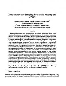
6.2. Tracking examples A typical example of the tracking results achieved with the SBF-IS algorithm is depicted in Figure 1. It contains the plots of the estimated source position versus time resulting from the two PF methods. The grey lines above and below the estimated source position represent plus/minus one standard deviation of the particle set for both the xand y-coordinates. The audio data used in this example was recorded in a real office room with reverberation time T60 = 0.39 second and average SNR 9.4 dB. The acoustic source was moving at a constant speed along a straight line over a distance of about 1.6 m. The signal recorded with one of the array sensors is given as an example in Figure 1(a). This practical result also demonstrates the reinitialisation capabilities of the IS method, with the set of particles purposely initialised in a random room location at the start of the simulation, about 2 m away from the true start position of the target. As soon as the source starts emitting an acoustic signal, the IS method is able to relocate its particles towards the true source position and subsequently tracks the target as it moves across the state space. The non-IS filter is unable to detect the source due to the current measurement data not being taken into

1

2

3

4

5

6

7

5

6

7

5

6

7

5

6

7

5

6

7

Time (s) (a) x-position (m)

The setup defined for the following experiments was based on a medium-sized room measuring roughly 2.9 m × 3.8 m × 2.7 m, and fitted with an array of M = 8 omnidirectional microphones positioned at a constant height and organised as one pair on each wall. In each pair, the distance between the sensors was 0.6 m. The microphone signals used in the experiments were samples of audio data sampled at 8 kHz, either recorded in a real office room or generated using the image method [18]. For the practical recordings, the sound source was simulated with a loudspeaker moving along a predefined path across the enclosure. The signals were split into frames of 512 samples (processed using a Hamming window), and subsequently used as observation to compute both the importance and likelihood functions. The data processing was carried out using a 50% overlapping factor, yielding the update interval TU = 0.032 second. The numerical values defined for the transition model parameters were set to v = 0.7 m/s and β = 10 Hz. For the SBF-IS algorithm, the importance function was computed over a horizontal grid of points uniformly distributed across the state space with a spacing of 0.1 m. In the following results, the performance of the IS algorithm is compared to that of the SBF-PL method, a bootstrap-only algorithm described in [3]. For both methods, the number of particles was set to N = 30. Other algorithm-specific parameters were optimised empirically to achieve a satisfactory tracking performance, using a reference sample of real-audio data recorded in the environment described above.

2 1 0 1

2

3

4 Time (s)

(b) y-position (m)

6.1. Experimental setup

0.2 0.1 0 −0.1 −0.2

3 2 1 0 1

2

3

4 Time (s)

(c) x-position (m)

PRACTICAL EXPERIMENTS

2 1 0 1

2

3

4 Time (s)

(d) y-position (m)

6.

EURASIP Journal on Applied Signal Processing

3 2 1 0 1

2

3

4 Time (s)

(e)

Figure 1: Tracking results obtained with an IS-based and a non-IS method. (a) Example of signal recorded with one array sensor for this simulation. (b)–(e) True source position (dotted lines), source location estimate (solid lines), and lines representing ± one standard deviation of the particle set (grey lines). (b), (c) SBF-PL. (d), (e) SBF-IS.

account when propagating the particles. The situation described in Figure 1 typically constitutes an example of target detection (track acquisition), for which the IS method clearly shows its superiority over a pure bootstrap implementation. More results on the tracking performance of algorithm SBFPL can be found in [3].

E. A. Lehmann and R. C. Williamson

7

0.02 0.01 0 −0.01 −0.02

0.5

1

1.5 2

2.5 3

3.5 4

4.5 5

5.5

4.5 5

5.5

4.5 5

5.5

Time (s)

x-position (m)

(a)

2 1 0 0.5

1

1.5 2

2.5 3

3.5 4

Time (s)

y-position (m)

(b)

3 2 1 0

0.5

1 1.5 2

2.5 3

3.5 4

Time (s) (c)

Figure 2: SBF-IS tracking results with alternating conversation scenario. (a) Example of audio signal generated for one of the array sensors. Vertical dotted lines denote a change of speaker. (b), (c) Tracking results in x- and y-coordinates. Dotted lines represent the position of the active source.

The results depicted in Figure 2 were obtained with a scenario where two speakers take part in an alternating conversation. The simulation was carried out using the image method to generate signals originating from two different locations in the above mentioned setting, with a reverberation time T60 = 0.35 second. White noise was added to the microphone signals with an SNR level of about 20 dB. Figure 2(a) shows an example of signal resulting for one of the sensors. The vertical dotted lines represent time instants at which a speaker change occurs in the original source signal. Figures 2(b) and 2(c) show the tracking results obtained with the SBF-IS algorithm. This demonstrates once again the efficiency of this method which automatically switches between talkers as soon as a speech signal is detected at a different location in the state space. 6.3. Image method results Results presented in the previous section specifically demonstrate the performance of the IS algorithm during the phase of target detection, that is, in localisation mode. This section deals with a more specific assessment of the PF operating in tracking mode only. To this purpose, the particles were initialised at the true source location at the beginning of each simulation in the following results.

For this experiment, the microphone signals were generated with the image method [18] for varying values of reverberation time T60 . White noise was added to the resulting signals with an approximate SNR level of 20 dB. A single example of target trajectory and source signal was considered, with a path corresponding to a 1.6 m straight line across the room. The source signal was a sentence uttered by a male speaker, defining a 7.3- second audio sample. The results presented in Figure 3 were obtained by simulating each PF algorithm 100 times for the considered audio data. For each run, an estimate of the tracking accuracy was computed as the average deviation (root mean squared error (RMSE)) of the PF location estimate from the true source trajectory. The statistical distribution of this assessment parameter (for each value of T60 ) is plotted in Figure 3 using a boxplot representation, which contains information about interquartile range and median of the RMSE data set. For low to medium reverberation times, that is, up to T60 ≈ 0.6 second, these results show that the median tracking accuracy of both IS-based and non-IS methods is similar. Simulation runs for which the PF does not recover after losing track of the target result in the appearance of a second mode in the distribution of the RMSE parameter. This effect can be seen easily in the SBF-PL results for reverberation times greater than about 0.4 second, whereas the reinitialisation capabilities of the SBF-IS method allow such cases to be mostly avoided. On the other hand, SBF-IS algorithm exhibits distributions of the RMSE results that are more spread out: the outliers appear here as the tail of the distribution rather than a separate mode. This results from the SBF-IS algorithm occasionally reinitialising off-track (i.e., erroneously) and then recovering, rather than due to a complete and definitive loss of the target as with SBF-PL. 6.4.

Further discussion

When designing any tracking algorithm, a compromise must be found between its localisation ability and its tracking accuracy. With the proposed IS algorithm, this can be achieved very efficiently by tuning the prior probabilities of the reinitialisation and importance sampling options, P R and P S , respectively. A bootstrap implementation constitutes an extreme limit in this tradeoff with P R = P S = 0. On the basis of a (nonoptimised) Matlab implementation, it can be seen that the SBF-IS algorithm requires roughly twice more computational power than SBF-PL to process the same amount of input data. This is of course due to the additional task of computing the importance function over a fixed grid of points across the state space. However, a real-time implementation of the SBF-IS algorithm, running on a 1.7 GHz computer in conjunction with a 16-sensor array, shows that this additional processing power requirement does not represent any difficulties for modern desktop computers. Given this hardware setup, the number of particles in the IS algorithm can be increased up to 120 before reaching the limits of the system resources, which proves to be more than sufficient for the considered application. This practical implementation demonstrates the robustness of the

EURASIP Journal on Applied Signal Processing

RMSE (m)

8

algorithm would typically necessitate additional processing units to deal with such scenarios, whereas the IS method already integrates these functionalities at a low level in the algorithm.

1 0.5

ACKNOWLEDGMENTS

0 0 0.06 0.13 0.21 0.28 0.35 0.42 0.50 0.57 0.64 0.71 0.79 T60 (s)

RMSE (m)

(a)

1 0.5

REFERENCES

0 0 0.06 0.13 0.21 0.28 0.35 0.42 0.50 0.57 0.64 0.71 0.79 T60 (s) (b)

Figure 3: Statistical tracking performance results obtained with simulated reverberant data (image method) for various levels of reverberation. In each boxplot, the dots represent RMSE data points, the lines at the top and bottom of the box correspond to the 75th and 25th percentile of the data set, respectively, and the horizontal line in the middle of the box is the median of the data set. (a) SBF-PL. (b) SBF-IS.

IS algorithm when localising sources and tracking fast target motions in the setting of a 3.5 m × 4.5 m × 2.7 m office room with a practically measured reverberation time T60 = 0.5 second. Demonstration movies (originally recorded in real time) showing some typical examples of the IS algorithm output delivered by this implementation can be found online at DOI 10.1155/ASP/2006/17021. Finally, it must be kept in mind that the tracking performance of the IS method developed in this paper can be potentially largely improved by using some additional information (such as, e.g., voice activity detection) to adjust the reinitialisation probability P R . The use of a more elaborate beamforming principle providing improved localisation estimates would also lead to a better tracking performance. 7.

This paper was performed while Eric A. Lehmann was working with National ICT Australia. National ICT Australia is funded by the Australian Government’s Department of Communications, Information Technology, and the Arts, the Australian Research Council, through Backing Australia’s Ability, and the ICT Centre of Excellence programs. We would also like to thank the reviewers for their comments.

CONCLUSION

Speaker localisation and tracking are complicated array processing applications, made especially challenging by complex reverberation effects and the discontinued nature of speech signals. Adopting a Bayesian filtering approach to this problem leads to superior tracking performance compared to traditional acoustic localisation methods. In this paper, we have developed a particle filtering technique using the principle of importance sampling. The resulting algorithm is able to automatically recover from track loss, detect a new source entering the acoustic scene, and switch between speakers taking turns, thus making it more suitable than bootstrap methods in practise. In a practical tracking system, a bootstrap-only

[1] T. G. Dvorkind and S. Gannot, “Speaker localization exploiting spatial-temporal information,” in Proceedings of International Workshop on Acoustic Echo and Noise Control (IWAENC ’03), pp. 295–298, Kyoto, Japan, September 2003. [2] J. Vermaak and A. Blake, “Nonlinear filtering for speaker tracking in noisy and reverberant environments,” in Proceedings of IEEE International Conference on Acoustics, Speech, and Signal Processing (ICASSP ’01), vol. 5, pp. 3021–3024, Salt Lake City, Utah, USA, May 2001. [3] D. B. Ward, E. A. Lehmann, and R. C. Williamson, “Particle filtering algorithms for tracking an acoustic source in a reverberant environment,” IEEE Transactions on Speech and Audio Processing, vol. 11, no. 6, pp. 826–836, 2003. [4] D. B. Ward and R. C. Williamson, “Particle filter beamforming for acoustic source localization in a reverberant environment,” in Proceedings of IEEE International Conference on Acoustics, Speech, and Signal Processing (ICASSP ’02), vol. 2, pp. 1777– 1780, Orlando, Fla, USA, May 2002. [5] J. DiBiase, H. Silverman, and M. Brandstein, “Robust localization in reverberant rooms,” in Microphone Arrays: Signal Processing Techniques and Applications, M. Brandstein and D. B. Ward, Eds., pp. 157–180, Springer, Berlin, Germany, 2001. [6] C. Knapp and G. Carter, “The generalized correlation method for estimation of time delay,” IEEE Transactions on Acoustics, Speech, and Signal Processing, vol. 24, no. 4, pp. 320–327, 1976. [7] J. Benesty, “Adaptive eigenvalue decomposition algorithm for passive acoustic source localization,” Journal of the Acoustical Society of America, vol. 107, no. 1, pp. 384–391, 2000. [8] D. B. Ward, “Nonlinear filtering of the generalized crosscorrelation function for source localization,” in Proceedings of IEE Workshop on Nonlinear and Non-Gaussian Signal Processing, Peebles Hydro, UK, July 2002. [9] N. J. Gordon, D. J. Salmond, and A. F. M. Smith, “Novel approach to nonlinear/non-Gaussian Bayesian state estimation,” IEE Proceedings F Radar and Signal Processing, vol. 140, no. 2, pp. 107–113, 1993. [10] A. Doucet, S. Godsill, and C. Andrieu, “On sequential Monte Carlo sampling methods for Bayesian filtering,” Statistics and Computing, vol. 10, no. 3, pp. 197–208, 2000. [11] M. S. Arulampalam, S. Maskell, N. Gordon, and T. Clapp, “A tutorial on particle filters for online nonlinear/non-Gaussian Bayesian tracking,” IEEE Transactions on Signal Processing, vol. 50, no. 2, pp. 174–188, 2002. [12] A. Doucet, N. de Freitas, and N. Gordon, Eds., Sequential Monte Carlo Methods in Practice, Springer, New York, NY, USA, 2001.

E. A. Lehmann and R. C. Williamson [13] J. Vermaak, M. Gangnet, A. Blake, and P. P´erez, “Sequential Monte Carlo fusion of sound and vision for speaker tracking,” in Proceedings of 8th IEEE International Conference on Computer Vision (ICCV ’01), vol. 1, pp. 741–746, Vancouver, BC, Canada, July 2001. [14] M. Isard and A. Blake, “ICONDENSATION: Unifying lowlevel and high-level tracking in a stochastic framework,” in Proceedings of 5th European Conference on Computer Vision (ECCV ’98), vol. 1, pp. 893–908, Freiburg, Germany, June 1998. [15] E. A. Lehmann, D. B. Ward, and R. C. Williamson, “Experimental comparison of particle filtering algorithms for acoustic source localization in a reverberant room,” in Proceedings of IEEE International Conference on Acoustics, Speech, and Signal Processing (ICASSP ’03), vol. 5, pp. 177–180, Hong Kong, April 2003. [16] M. Brandstein and D. B. Ward, Eds., Microphone Arrays: Techniques and Applications, Springer, Berlin, Germany, 2001. [17] B. Ristic, S. Arulampalam, and N. Gordon, Beyond the Kalman Filter: Particle Filters for Tracking Applications, Artech House, Boston, Mass, USA, 2004. [18] J. Allen and D. Berkley, “Image method for efficiently simulating small-room acoustics,” Journal of the Acoustical Society of America, vol. 65, no. 4, pp. 943–950, 1979. Eric A. Lehmann graduated in 1999 from the Swiss Federal Institute of Technology in Zurich (ETHZ), Switzerland, with a Diploma in electrical engineering (Bachelor equivalent). He received the M.Phil. and Ph.D. degrees, both in electrical engineering, from the Australian National University, Canberra, in 2000 and 2004, respectively. After working as a Research Engineer for National ICT Australia (NICTA) in Canberra, he is now a Research Fellow with the Western Australian Telecommunications Research Institute (WATRI) in Perth, Australia. His current scientific interests include acoustics, signal and speech processing, microphone arrays, and Bayesian estimation and tracking, with particular emphasis on the application of sequential Monte Carlo methods (particle filters). Robert C. Williamson received the B.E. degree (electrical engineering) from the Queensland University of Technology in 1984 and the Master’s of Engineering Science degree (electrical engineering) from the University of Queensland in 1986. In 1990 he obtained the Ph.D. degree in electrical engineering from the University of Queensland. He joined the Australian National University as a Postdoctoral Fellow in the Department of Systems Engineering in 1990 and held a series of appointments before becoming a Professor in the Computer Sciences Laboratory, Research School of Information Sciences and Engineering. He is NICTA’s Chief Researcher, an Advisory Board Member of the Australian Communications Research Network, a Director of Epicorp, and a Member of the Editorial Board of the Journal of Machine Learning Research. His scientific interests include signal processing and machine learning.

9

Photographȱ©ȱTurismeȱdeȱBarcelonaȱ/ȱJ.ȱTrullàs

Preliminaryȱcallȱforȱpapers

OrganizingȱCommittee

The 2011 European Signal Processing Conference (EUSIPCOȬ2011) is the nineteenth in a series of conferences promoted by the European Association for Signal Processing (EURASIP, www.eurasip.org). This year edition will take place in Barcelona, capital city of Catalonia (Spain), and will be jointly organized by the Centre Tecnològic de Telecomunicacions de Catalunya (CTTC) and the Universitat Politècnica de Catalunya (UPC). EUSIPCOȬ2011 will focus on key aspects of signal processing theory and applications li ti as listed li t d below. b l A Acceptance t off submissions b i i will ill be b based b d on quality, lit relevance and originality. Accepted papers will be published in the EUSIPCO proceedings and presented during the conference. Paper submissions, proposals for tutorials and proposals for special sessions are invited in, but not limited to, the following areas of interest.

Areas of Interest • Audio and electroȬacoustics. • Design, implementation, and applications of signal processing systems. • Multimedia l d signall processing and d coding. d • Image and multidimensional signal processing. • Signal detection and estimation. • Sensor array and multiȬchannel signal processing. • Sensor fusion in networked systems. • Signal processing for communications. • Medical imaging and image analysis. • NonȬstationary, nonȬlinear and nonȬGaussian signal processing.

Submissions Procedures to submit a paper and proposals for special sessions and tutorials will be detailed at www.eusipco2011.org. Submitted papers must be cameraȬready, no more than 5 pages long, and conforming to the standard specified on the EUSIPCO 2011 web site. First authors who are registered students can participate in the best student paper competition.

ImportantȱDeadlines: P Proposalsȱforȱspecialȱsessionsȱ l f i l i

15 D 2010 15ȱDecȱ2010

Proposalsȱforȱtutorials

18ȱFeb 2011

Electronicȱsubmissionȱofȱfullȱpapers

21ȱFeb 2011

Notificationȱofȱacceptance SubmissionȱofȱcameraȬreadyȱpapers Webpage:ȱwww.eusipco2011.org

23ȱMay 2011 6ȱJun 2011

HonoraryȱChair MiguelȱA.ȱLagunasȱ(CTTC) GeneralȱChair AnaȱI.ȱPérezȬNeiraȱ(UPC) GeneralȱViceȬChair CarlesȱAntónȬHaroȱ(CTTC) TechnicalȱProgramȱChair XavierȱMestreȱ(CTTC) TechnicalȱProgramȱCo Technical Program CoȬChairs Chairs JavierȱHernandoȱ(UPC) MontserratȱPardàsȱ(UPC) PlenaryȱTalks FerranȱMarquésȱ(UPC) YoninaȱEldarȱ(Technion) SpecialȱSessions IgnacioȱSantamaríaȱ(Unversidadȱ deȱCantabria) MatsȱBengtssonȱ(KTH) Finances MontserratȱNájarȱ(UPC) Montserrat Nájar (UPC) Tutorials DanielȱP.ȱPalomarȱ (HongȱKongȱUST) BeatriceȱPesquetȬPopescuȱ(ENST) Publicityȱ StephanȱPfletschingerȱ(CTTC) MònicaȱNavarroȱ(CTTC) Publications AntonioȱPascualȱ(UPC) CarlesȱFernándezȱ(CTTC) IIndustrialȱLiaisonȱ&ȱExhibits d i l Li i & E hibi AngelikiȱAlexiouȱȱ (UniversityȱofȱPiraeus) AlbertȱSitjàȱ(CTTC) InternationalȱLiaison JuȱLiuȱ(ShandongȱUniversityȬChina) JinhongȱYuanȱ(UNSWȬAustralia) TamasȱSziranyiȱ(SZTAKIȱȬHungary) RichȱSternȱ(CMUȬUSA) RicardoȱL.ȱdeȱQueirozȱȱ(UNBȬBrazil)