Path Query Processing on Very Large RDF Graphs Andrey Gubichev
Thomas Neumann
Technische Universität München Germany
[email protected]
Technische Universität München Germany
[email protected]
ABSTRACT Finding the shortest path between two nodes in an RDF graph is a fundamental operation that allows to discover complex relationships between entities. In this paper we consider the path queries over graphs from a database perspective. We provide the full-fledge database solution to execute path queries over very large RDF graphs. We present low-level techniques to speed-up shortest paths algorithms, and a robust method to estimate selectivities of path queries. We perform extended experiments on several large RDF collections, including the UniProt collection, demonstrating that our approach outperforms the path query capabilities of modern systems by a large margin.
1.
INTRODUCTION
The RDF data format, designed to represent data for the Semantic Web, has become a common format for building large data collections. In particular, biological and knowledge management communities use RDF-based representation of their data. RDF provides certain flexibility for querying that the relational model does not offer: the RDF dataset is queried by matching patterns in the RDF graph, where property names, the RDF counterparts of relational attributes, can be left unspecified in a schema-agnostic, ’pay as you go’ manner. However, even with such expressive capabilities, the standard RDF query language SPARQL does not support discovery of complex relations between RDF objects. One of the commonly needed types of relationships is reachability. Object A is reachable from object B in the RDF graph if there exists a path from B to A. We refer to the queries that return reachable objects together with corresponding shortest paths as path queries. The need for path queries is easily identifiable in many applications and has been investigated in several contexts ranging from national security [19] to genome biology [16]. Here we present a common scenario of path query usage in the area of knowledge management.
Copyright is held by the author/owner. Fourteenth International Workshop on the Web and Databases (WebDB 2011), June 12, 2011 - Athens, Greece .
Let us consider the information about two scientists that is presented in the (subject, predicate, object)-triple form: (Albert Einstein, bornIn, Ulm) (Alexander von Humboldt, bornIn, Berlin) (Ulm, locatedIn, Baden-W¨ urttemberg) (Baden-W¨ urttemberg, locatedIn, Germany) (Berlin, locatedIn, Germany) Here, the relation between Albert Einstein and Germany can be expressed with the path (Albert Einstein, bornIn, Ulm, locatedIn, Baden-W¨ urttemberg, locatedIn, Germany), and the natural query to ask is Find all the scientists that were born in Germany. This query requires matching all entities–places that can reach Germany via several locatedIn predicates, and then finding the entities–persons that are related with the bornIn predicate to that entities–places. Note that, in principle, we would be able to translate this query into the standard SPARQL disjunctive query (with union and several potentially long chain joins), if we knew the length of the paths and the exact schema in advance. However, this assumption contradicts the schema-free or schema-later nature of RDF data, since it requires a priori knowledge about the path structure. Path queries help to investigate complex relationships between entities in a variety of cases, starting from the simple question How is Thomas Mann related to Leo Tolstoy? to the quite sophisticated Find all South-European born scientists that became known for any physics-related discoveries. In the first case the related to connection can be expressed as the path in the graph, while in the second case we have two such relations: place of birth to South Europe, and specific discovery to physics. Apart from knowledge management, path queries are particularly useful for biological applications. The reachability via the path in the biological datasets corresponds to biological interactions, for example between genes or pathways. Here, researchers are interested not only in reachable objects, but also in the paths as such (interaction networks). Path query processing on large-scale data includes several technical challenges. First, extremely efficient execution of physical operators (simple path queries) is required, since later they are used as building blocks for complex star- and chain-shaped join queries. Second, optimization of complex join queries per se calls for accurate estimation of selectivities for the path queries. The main contributions of this paper are: • At a low level, we introduce techniques allowing us to significantly (by a factor of 10) speed up Dijkstra’s shortest path algorithm (and also other shortest path algorithms) by carefully choosing the physical layout
of the graph and graph-based operations. • At a higher level, we present a simple yet powerful way to estimate the selectivity of queries with paths, enabling cost-based query optimization. • We provide an integrated solution that puts all these techniques together for RDF path query processing. • We give an extensive experimental analysis of our techniques using the very large RDF graphs of UniProt and YAGO2. We demonstrate that our solution outperforms the Jena system [1] by several orders of magnitude. We implemented our techniques in the open-source system RDF-3X [2]. The rest of the paper is organized as follows. In Section 2 we overview the previous approaches to path query processing. Then, in 3.1, we briefly describe the SPARQL extension with path query patterns, and review the RDF query processing system that we build upon in 3.2. We present our fast shortest path algorithm based on Dijkstra’s algorithm in 3.3. We proceed with low-level techniques for dictionary organization in the RDF engine (3.4), and selectivity estimations of path queries (3.5). We present the implementation details of the RDF-path query system and the experimental results in Section 4.
2.
RELATED WORK
There are several lines of work related to path queries on graphs. Reachability and shortest path problems have been intensively studied in the database community. A survey of this research can be found in [5]. Approximate shortest paths were also considered in the prior work [18, 11]. The approach pursued in this paper is orthogonal to this line of work. We take the classical Dijkstra’s shortest path algorithm, and build a full-fledged path query processing system on it. Besides, we propose low level database techniques which speed up Dijkstra’s algorithm on disk-resident graphs, that can be applied to other shortest-path algorithms as well. The languages for path queries over graph-structured data have been the subject of much investigation in the theoretical community. The most recent survey was done by Barcelo et al.[9]. In this work we use a query language similar to SPARQ2L [8]. Several frameworks and prototypes for RDF path queries have been proposed. Namely, Anyanwu et al. [8] propose a path query evaluation framework, that relies on expensive matrix decomposition for the precomputation step (O(n3 ), where n is the number of nodes in the RDF graph) and therefore cannot scale to real-world big graphs. The GRIN engine [20] concentrates on providing an index for graph queries utilizing graph partitioning, but the construction time for such an index is also prohibitively long (O(n4 log n)). BRAHMS [14] is another example of an engine that supports graph traversal queries. However, it only finds the paths with a predefined (fixed) length. DOGMA [10] is a disk-based graph pattern matching index, but it does not support path query processing. Note that all past work on RDF path query processing has the following limitations: (i) algorithms for query processing are all main-memory based, and do not include any implementation details or large-scale experiments, (ii) there is no work on selectivity estimation and path query optimization.
Finally, to the best of our knowledge, Jena [1] is the only mature RDF engine that supports path queries on diskresident graphs as an extension to the standard SPARQL. However, as we show in the experiments section, the performance of the system is very poor.
3. 3.1
PATH QUERY PROCESSING Extension of SPARQL
In this section we describe the extension of the SPARQL query language that allows us to query paths in RDF database. Let I, L, B be the pairwise disjoint sets of URIs, literals and blank nodes, respectively. A dataset G is a set of triples hs, p, oi, where s is the Subject, p is the Predicate, and o is the Object. A subject can be a unique identifier from I ∪ B, a predicate can only be a URI from I, an object can be an identifier from I ∪ B or a literal L. The set of triples naturally forms a directed edge labeled RDF graph, where nodes correspond to subjects and objects, and edges are labeled with predicates. An RDF path (or simply a path) of length n from a node x to a node y in an RDF graph is an ordered sequence of triples hx, p1 , o1 ihs2 , p2 , o2 i · · · hsn+1 , pn+1 , yi, where oi = sj+1 for 1 ≤ i ≤ n − 1. A basic SPARQL query has the form select ?var1 ?var2... where {pattern1. pattern2...} where each pattern is an hs, p, oi triple, and each of s,p and o is either a variable, or a constant from the corresponding domain. Following W3C recommendations, we start the names of the variables with ’ ?’. In tune with previous work [7, 8, 15], we enrich the SPARQL syntax with a path triple pattern. Path triple patterns resemble the standard SPARQL triple pattern, but they contain a path variable in the predicate position. We will distinguish between regular and path variables by starting the latter with ’ ??’. A path variable in the path triple matches the shortest path from a subject to an object in the RDF graph. For example, the path pattern ??path ?var2 matches all the objects reachable from and the shortest paths from to all such objects. Multiple triple patterns are combined in a conjunctive manner and can share regular variables, thus implying joins. We recursively define any (regular or path) triple pattern as bounded, if (i) either subject or object is constant, or (ii) it shares at least one variable with a bounded pattern. For example, the path pattern in the following group of patterns is bounded: ?person ??path ?city. ?city ?country. ?country In this work we restrict ourselves to bounded path patterns. Informally this means that the query engine always knows the set of values of either subject or object in the path triple and thus does not have to consider all-to-all shortest paths during query execution. Similarly to [8], we also allow the specification of filter conditions on path variables. The filter condition can be constructed from several built-in functions, arithmetic and boolean operators (=,≤, & ,∨). Let V R and V P be the set of regular and path variables correspondingly. We added the
Algorithm 1: Join-based Dijkstra’s algorithm Input: s, d - start and destination nodes in the graph Result: path p from s to d 1 begin 2 Q ← {s} 3 Vcur ← {s} 4 Vprev ← ∅ 5 while Q is not empty do 6 node ← Q.dequeue 7 node.status ← processed 8 if node = d then 9 p ← reconstruct path from s to d 10 11 12 13 14 15 16 17
if Vprev is empty then S ← getNeighbors(Vcur ) Vprev ← Vcur clear Vcur Remove node from Vprev Relax nodes from S[node] foreach n ∈ S[node],n.status 6=processed do Add node to Vcur
5 8
2 6 3 1
7 4
Figure 1: Dijkstra’s algorithm
function containsAny(path, element), where path ∈ V P and element ∈ V R, that checks whether path contains node or edge element. The function containsOnly(path, element) with the same domains checks whether path consists only of element. In this case path can be seen as sequence of zero or more element. Finally, the function length(path) returns the length of path, and together with comparison operations it allows us to restrict the length of the path. Syntactically, the path filter conditions are used in the same way as filter in SPARQL.
3.2
RDF query processor
We assume a system architecture, where each Subject, Predicate and Object from every RDF triple is mapped to an integer and stored in a global dictionary. All six possible permutations of S, P and O should be indexed in six separate B+ -trees. This indexes contain the triples themselves instead of references to the triples. Each index can be significantly compressed by delta-coding of triples. Moreover, there are merge and hash joins that operate directly on triple indexes. Finally, the query optimizer chooses a cost-model-based execution plan. All this is available in the RDF-3X engine [17]. Other RDF engines provide some of these features, the rest can be implemented with reasonable programming effort. In order to support our extended SPARQL, we need to provide a system with ability to find paths and reachable nodes and to estimate the selectivity of the queries.
3.3
Join-based Dijkstra’s algorithm
We build our path query processor upon the classical Dijkstra’s algorithm [12]. The algorithm finds the shortest path
S P O ... 2
1
0
4
2
0
3
2
0
5
3
2
0
6
4
3
0
4
3
0
4
0
Edge Succ
⇒
0
3
0
5
0
6
0
4
6
0
6
7
0
7
... Figure 2: Join-based getNeighbors
between two nodes by traversing nodes in the graph in a breadth-first manner. Trivial modifications to Dijkstra’s algorithm allow us to find the paths from the source to every other node in the graph, or to construct shortest path trees with several sources. Since the graph is disk-resident, for every visited node the algorithm needs to retrieve the list of its successors from disk. We will call this operation getNeighbors. A naive approach to perform getNeighbors for all visited nodes is to execute it independently for every node. Namely, for every visited node u we initiate a scan on the SPO index, look up the position of u in the corresponding B+ -tree, read the leaf and decompress it, and extract all triples that have u as a subject from the decompressed leaf. We can get the reverse Dijkstra’s algorithm simply by scanning the OPS index, in this case at every step we get the predecessors of each processed node. However, this multiple-lookup based implementation becomes the bottleneck of the algorithm for disk-resident graphs. Consider, for example, the graph in Figure 1. The start node is 1, and we enqueue all its successors. Then, we issue three different requests to disk to get the successors of the nodes 2,3,and 4. This results in three B+ -tree lookups. Even if all three nodes reside on the same leaf page, we will read and decompress it three times. Caching the page would solve this particular problem, but it does not scale well since the number of nodes (and pages) grows exponentially. We can speed up this process by getting the successors of all three nodes in one database request. Namely, let us think of a pseudo-scan operator that iterates over nodes 2, 3 and 4. If we join this operator with an SPO-index scan of the whole database, we will get all the triples that start with 2, 3 and 4 respectively, i.e. exactly the successors of the nodes in consideration. Figure 2 gives an illustration of this idea. We join on the S-column and return values from P and O columns (labels of the edges and successors, respectively). The join (actually, the merge join) is faster than the multiple lookups due to several reasons: First, while merging, the RDF engine locates the B+ -tree leaf containing the first node, and then scans the sequence of leaves, occasionally skipping those that a priori can not contain nodes of interest. Second, if the input nodes are located on the same leaf page, we will read and decompress this page only once, as opposed to the multiple extractions done by multiple-lookup approach. Third, by combining several nodes in one request, we significantly reduce the number of total requests to disk. Our join-based getNeighbors operation takes the set of nodes as an input, therefore we need to accumulate several visited nodes prior to calling it. This idea is leveraged by Join-based Dijkstra’s algorithm, sketched in Algorithm 1. The algorithm alters the standard Dijkstra’s algorithm in the following way: 1. We collect visited nodes in Vcur and later use them as an input for the getNeighbors operation. The nodes that were used for the previous call of getNeighbors,
are kept in Vprev . 2. As the traversal proceeds, the new nodes are added to Vcur , and the scanned nodes are deleted from Vprev . 3. Once Vprev becomes empty, we need to get the new portion of neighbors. The nodes that were queued in Q since the last getNeighbors operation (we store them in Vcur ) become an input for the new join-based getNeighbors operation. Consider, for example, the graph in Figure 1. We start the computation with Vcur = {1}. Since we do not have any nodes in our buffer S, we get the successors for the nodes in Vcur . Nodes 2, 3 and 4 are now enqueued and added to Vcur , and node 1 is removed from Vprev (indicating that for the next loop we need to load new portion of successors). Now, we request the successors for Vcur = {2, 3, 4} and continue the usual Dijkstra processing until we reach node 4 and delete it from Vprev . After that we again request the successors for Vcur = {5, 6, 7}, and so on. Every time the set of nodes that are processed in the getNeighbors is a new layer of the graph depicted with dashed lines in Figure 1. Naturally, these additional operations on Vprev and Vcur can be done in O(log n), thus leaving the overall complexity O(n log n + m), where n and m is the number of nodes and edges, respectively. As shown later, however, the join-based Dijkstra’s algorithm is an order of magnitude faster than the original one. It is worth pointing out that the join-based technique of getting successors of several nodes can be employed by other shortest paths algorithms, including A∗ , reach and landmark -based approaches [6, 13]. There are two main advantages of the Dijkstra’s algorithm: (i) it finds shortest paths and not only reachable nodes, and (ii) it does not incur any preprocessing overhead. We therefore employ it as the main physical operator for path queries and leave the investigations of more efficient algorithms for the future work.
3.4
Dictionary
RDF-3X assigns an integer ID to every URI and string constant, and operates on triples of integers. The ID-toliteral mapping is maintained in the global dictionary, which can be implemented as a B+ -tree or a directed mapping index [17]. In both cases, strings with close IDs reside on adjacent pages, or even within one page. The assignment of IDs is done during the data loading on a First-Come, First-Served basis. In this case, the successors of one node can get IDs that are far away from each other. It can happen, for example, when the triples with the same subject are scattered in the input file. Recall the example in Figure 1. Suppose that the graph depicted there is a subgraph of a much larger graph, such that the nodes 2, 3, 4 were assigned internal ids 20, 50, and 100 respectively. Suppose also that every leaf of the B+ -tree SPO index contains 10 entries (every entry is a triple). In this case, entries corresponding to the 2, 3, 4 nodes are far away from each other in the SPO index, and the getNeighbors operation will be likely to read three different leaves from disk when applied to {2, 3, 4}. The problem will become worse in the next iterations, when the number of input nodes increases. Another problem with First-Come, First-Served assignment is mapping the results of the path query execution back from IDs to strings. If the successors of the same node have IDs far away from each other, we are likely to read another page for every next node. This leads to almost random
Algorithm 2: Dictionary 1 2 3 4 5 6 7 8 9 10 11 12
Result: new mapping id[n] for every node in the graph begin Sources ← set of nodes with no incoming edges curId = 0 foreach s ∈ Sources do id[s] = curId curId = curId + 1 Q ← {s} while Q is not empty do node = Q.dequeue if node does not have an id then id[node] = curId curId = curId + 1
13 14
get and relax neighbors add unprocessed neighbors to Q
ID-to-string lookups from disk, which becomes extremely inefficient for unselective queries. Both of these problems can be escaped by assigning IDs to nodes in the breadth-first order. Initially, we generate the temporary dictionary in a First-Come,First-Served manner, then we can still operate on triples of integers. We propose the procedure, presented in Algorithm 2, which operates on top of the temporary dictionary. It starts with finding all root nodes of the graph, i.e. nodes without incoming edges. From every root node s we run a breadth-first-search, assigning new IDs in the order of the search. If the node already has an ID, we skip it. This may happen if this node was processed during the breadth-first-search from a previous root. Final assignment of IDs is done before the strings are loaded, and before any index is created so that created indexes already contain triples with new, breadth-first-based IDs.
3.5
Cardinality estimation
Regardless of the path query processing on the physical level, advanced path queries over huge RDF graphs require cardinality (and thus selectivity) estimation for path triples for query optimization. In this section we discuss estimators for individual path triples, which can be indexed when the data is loaded. Then, the runtime selecitivity estimation merely requires one or two lookups in a small-sized B+ -tree, which is neglible compared to the actual query execution time. We first consider the case when the path triple pattern (s, p, o) contains one constant node (subject s or object o). Then, the cardinality estimation of such a triple pattern boils down to computing the number of nodes visited by Dijkstra’s algorithm starting from s or reversed Dijsktra’s algorithm starting from o. The procedure estimating this number is given in Algorithm 3. We start from the nodes in RDF graph that do not have any successors (’leaves’). Then, we run breadth-first-traversal in the reversed edges direction (lines 3-8), that is, going ’up’ the graph. For every visited node, we already know the forward selectivity of all its successors since we visited them before processing the current node, so we just sum up their estimations with the number of successors and get the estimation f orward[node] (lines 6-8). We proceed with the backward estimation in the same manner (lines 9-15). The results of this procedure are materialized in the B+ -tree indexed by the constant included in the pattern.
Algorithm 3: Cardinality estimation Result: forward[n], backward[n] - cardinality of Dijkstra and reversed Dijkstra for every node 1 begin 2 S ← set of nodes with literal-only successors or without successors 3 while do reversed Breadth-First Traversal from S do 4 foreach node visited do 5 Succ ← list of successors for node 6 foreach i ∈ Succ do 7 f orward[node]+ = f orward[i] f orward[node]+ = Succ.size
8
14
F ← set of nodes with no predecessors while do Breadth-First Traversal from F do foreach node visited do P red ← list of predecessors for node foreach p ∈ P red do backward[node]+ = backward[s]
15
backward[node]+ = P red.size
9 10 11 12 13
Table 1: Path triple selectivity estimation error for the YAGO2 dataset Direction
min error
5% quantile
median error
95% quantile
max error
mean error
forward backward
0 0
0 0.039
0.5 0.16
4.02 4.25
70534 20.78
170.6 0.87
If both subject s and object o are constant, we approximate the cardinality with |f orward[s] − backward[o]|. The last scenario is a triple pattern P1 with three variables. According to our restriction from Section 3.1, such a triple should be bounded. This implies that there exists a (possibly long) join chain in the query from P1 to a triple P2 with a constant subject or object. If we start breadth-first traversal from the constant subject (object) of P2 , it will naturally reach the subject (object) of our triple. Therefore, the cardinality of P2 can serve as an approximation of the cardinality of P1 , and this scenario is reduced to the previous one. We measured the accuracy of Algorithm 3 by using the YAGO2 dataset from Section 4 and comparing the estimated cardinalities with the real cardinalities. The test workload contains 1000 random triple patterns with one constant element (subject or object), the error of the approximation is max(real cardinality,estimation) −1. The results relative error = min(real cardinality,estimation) are shown in Table 1. On average (median error) we misestimate the backward selectivity by 16% and the forward selectivity by 50%. It takes 5 minutes to compute the new indexes, and they occupy 320 Mb on disk. This extra cost is just 10% of the database build time ( 45 minutes) and 12% of the disk space (2.5 Gb). On the other hand, as a result, cardinality estimation allows us to incorporate path query processing into RDF-3X cost model and query optimization [17].
4.
IMPLEMENTATION AND EVALUATION
We used the open-source system RDF-3X as a testbed for our techniques and augmented the query execution system to support path triple patterns. After parsing the query, every path triple pattern is translated into the special operator DijkstraScan that corresponds to the join-based Dijkstra algorithm with one or several start/stop nodes. This special operator is included into the query plan, and its selectivity is estimated according to Section 3.5. After that the query optimizer chooses the cheapest plan similarly to the pure
SPARQL case. If the subject or the object of the path triple is constant, then DijkstraScan is executed as join-based Dijkstra (reversed Dijkstra) in an asynchronous manner, like any other operator in RDF-3X. If both the subject and the object are query variables, the optimizer picks one of them depending on the selectivity. In this case the DijkstraScan operator starts with computing the set of subjects (objects), and then performs Dijkstra’s algorithm from this set. All experiments were performed on a 2-core Dell laptop with 4 Gb of memory using 64-bit Linux 2.6.35 kernel. We performed cold cache experiments by dropping all file-system caches and running the queries. We repeated this five times and measured the average response time for every query. For warm cache results we ran queries five times without dropping the caches. The SPARQL queries are given in the appendix. As the competitor for our system, we used the regular path processing in Jena [1] (GRIN and BRAHMS are not publicly available). We had to modify the syntax of queries to meet the syntax requirements of Jena. For the first experiment, we used the YAGO2 dataset [4] which consists of 80 million facts extracted from Wikipedia and integrated with the WordNet thesaurus. First, we evaluated the performance of the getNeighbors operation. We took 1000 random nodes, and for every node computed its successors and ran getNeighbors with the successors as the input, thereby getting all nodes that are 2 hops away from the random seed. We compared four different approaches: join-based algorithm vs. multiple lookup algorithm with two types of dictionary – the traditional RDF-3X dictionary and the one proposed in this paper. We also divide results into two groups, depending on how many nodes were returned by the operation. The obtained running times are provided in Table 3. It clearly identifies that the combination of the new dictionary and the join-based procedure yields the best running time for both scenarios. For the large output, this combination outperforms the naive approach (lookup with the old dictionary) by the factor of 10. However, if the number of nodes obtained from disk is relatively small, the difference between different techniques is not that big due to the join execution overhead. We also measured the runtimes of Dijkstra’s algorithm in the same four scenarios. Table 4 gives evidence that the proposed combination of clustered dictionary and join-based getNeighbors yields the best performance, outperforming the rest by an order of magnitude when the number of visited nodes is large. Then, we ran 5 different queries starting from the geographical hierarchy of Ulm (Q1) to all people from Germany that died somewhere in France(Q4) and all Mediterraneanborn European scientists that are known for some physical phenomenon(Q5). In general, the performance of Jena significantly degrades as the number of joins in the query increases. As reflected in Table 2, our approach outperforms Jena by a large margin, improving cold cache times by a factor of 32, and warm cache times by a factor of 27 in the geometric mean. RDF-3X was consistently better for all queries, gaining a factor of 1400 speed-up for the last query. To quantify how our individual techniques affect performance, we ran the experiments with the variants where only join-based Dijkstra and only new dictionary are used. The results are also presented in Table 5. As we see, both techniques play a significant role in ensuring high performance, gaining the speedup of a factor of 4.7 and 3 correspondingly in the cold cache case.
YAGO2
RDF-3X Jena
Q1
Q2
Q3
0.18 (0.004) 0.45 (0.1)
1.09 (0.19) 34.54 (1.31)
1.21 (0.09) 28.17 (1.07)
Q4
Q5 geom. mean cold cache (warm cache) 1.12 (0.18) 2.49 (1.39) 0.92 (0.11) 29.98 (0.95) >30min (>30min) >29.83 (>2.99)
Q1 0.52 (0.01)
UniProt Q2
Q3
geom. mean
4.01 (3.21) 11.54 (4.61) >30min (>30min)
2.88 (0.53)
Table 2: Query run-times in seconds for the YAGO2 and UniProt datasets Table 3: Runtime of getNeighbors operation less than 1000 nodes returned Dictionary new dict old dict
more than 1000 nodes returned
join
lookup
join
lookup
4 ms 18 ms
12 ms 13 ms
32 ms 78 ms
201 ms 228 ms
Table 4: Runtime of Dijkstra algorithm less than 1000 nodes visited Dictionary new dict old dict
more than 1000 nodes visited
join
lookup
join
lookup
5 ms 12 ms
8 ms 8 ms
120 ms 458 ms
1052 ms 1169 ms
For the second experiment, we used the UniProt dataset [3], which contains 57 GB of protein information. This dataset consists of 845 million unique triples. We ran three different queries with increasing number of joins in them. The results are given in Table 2. Jena also performs very poorly in this scenario. In fact, Jena was not able to evaluate any of the queries in 30 min., as opposed to the average response time of 2.88 seconds of RDF-3X.
5.
CONCLUSIONS
In this work we extended the RDF-3X system to support path queries over RDF. We significantly speeded up the classical Dijkstra’s algorithm by leveraging extremely fast join query processing in RDF-3X and by reorganizing the physical layout of the system’s dictionary. We pursued, for the first time, the query optimization approach for path queries and gave the algorithm for selectivity estimation of path triples. Our contributions achieve efficient performance on real datasets with 80 and 845 million triples. The proposed techniques are general and can be implemented in any RDF engine.
6.
[1] [2] [3] [4] [5]
[6]
[7] [8]
[9]
REFERENCES
Jena. http://jena.sourceforge.net/. RDF-3X. http://code.google.com/p/rdf3x/. Uniprot. http://dev.isb-sib.ch/projects/uniprot-rdf/. YAGO2. http://www.mpi-inf.mpg.de/yago-naga/yago/. C. C. Aggarwal and H. Wang. Managing and Mining Graph Data. Springer, 2010. R. Agrawal and H. V. Jagadish. Algorithms for searching massive graphs. IEEE Trans. on Knowl. and Data Eng., pages 225–238, 1994. K. Anyanwu. ρ-Queries: Enabling Querying for Semantic Associations on the Semantic Web. In WWW, 2003. K. Anyanwu, A. Maduko, and A. Sheth. SPARQ2L: Towards Support for Subgraph Extraction Queries in RDF Databases. In WWW, 2007. P. Barcelo et al. Expressive languages for path queries over graph-structured data. In PODS. ACM, 2010.
Table 5: Individual techniques (sec), YAGO2 dataset Direction
Q1
Q3
Q4
Q5
geom mean
baseline only new dict only join-based Dijkstra
cold cache 0.18 1.09 1.21 0.69 4.85 5.20 0.18 7.71 3.82
Q2
1.12 8.63 3.86
2.49 11.03 8.64
0.92 4.40 2.81
baseline only new dict only join-based Dijkstra
warm cache 0.004 0.19 0.09 0.04 0.99 0.75 0.004 0.41 0.29
0.18 0.54 0.36
1.39 5.87 4.86
0.11 0.62 0.24
[10] M. Br¨ ocheler, A. Pugliese, and V. S. Subrahmanian. Dogma: A disk-oriented graph matching algorithm for RDF databases. ISWC ’09. [11] A. Das Sarma et al. A sketch-based distance oracle for web-scale graphs. In WSDM. ACM, 2010. [12] E. W. Dijkstra. A note on two problems in connexion with graphs. Numerische Mathematik, 1(1):269–271, Dec. 1959. [13] A. V. Goldberg et al. Reach for A∗ : Efficient Point-to-Point Shortest Path Algorithms. In ALENEX, pages 129–143, 2006. [14] M. Janik and K. Kochut. BRAHMS: A WorkBench RDF Store and High Performance Memory System for Semantic Association Discovery . In ISWC, 2005. [15] K. J. Kochut and M. Janik. SPARQLeR: Extended SPARQL for Semantic Association Discovery. In ESWS, 2007. [16] W.-J. Lee et al. Using annotations from controlled vocabularies to find meaningful associations. DILS’07, 2007. [17] T. Neumann and G. Weikum. The RDF-3X engine for scalable management of RDF data. The VLDB Journal, 19:91–113, February 2010. [18] M. Potamias et al. Fast shortest path distance estimation in large networks. In CIKM, pages 867–876. ACM, 2009. [19] A. Sheth et al. Semantic association identification and knowledge discovery for national security applications. Journal of Database Management, 16:33–53, 2005. [20] O. Udrea, A. Pugliese, and V. S. Subrahmanian. GRIN: a graph based RDF index. In AAAI, 2007.
APPENDIX YAGO2 Q1. select ?loc ??path where { ??path ?loc. pathfilter( containsOnly(??path, )) } Q2. select ?obj where {?obj ??loc . ?obj . pathfilter(containsOnly( ??loc,))} Q3. select ?person where {?place ??loc . ?person ?place. ?person ?place. pathfilter(containsOnly(??loc,)) } Q4. select ?person where {?place1 ??loc1 . ?place2 ??loc2 . ?person ?place1. ?person ?place2. pathfilter(containsOnly(??loc1, ) && containsOnly(??loc2,))} Q5. select ?person where {?person ?smth. ?smth ??related . ?place ??loc ?country. ?country . ?country . ?person ?place.pathfilter(containsOnly(??loc, )) } UniProt Q1. select ?a ?mod ??inf where ?a ?vo. ?a . ?a . ?a ?mod. ?b ”2005-08-30”. ?b . ?b . ?a ?ab. ?ab ??inf ?b . Q2. select ?a ?vo where {?a ?vo. ?a . ?a . ?a ”1990-11-01”. ?a . ?a ??p ?b. ?b ”2005-08-30”. ?b . ?b ”false”. ?b ”true”. ?b } Q3. select ?a ?vo where {?a ?vo. ?a . ?a . ?a . ?a . ?a . ?b ”true”. ?b . ?b ”true”. ?b ”KPRS ECOLI”. ?b .?a ??p ?b }