Hindawi Publishing Corporation Mathematical Problems in Engineering Volume 2014, Article ID 642630, 19 pages http://dx.doi.org/10.1155/2014/642630
Research Article Path-Wise Test Data Generation Based on Heuristic Look-Ahead Methods Ying Xing,1,2 Yun-Zhan Gong,1 Ya-Wen Wang,1,3 and Xu-Zhou Zhang1 1
State Key Laboratory of Networking and Switching Technology, Beijing University of Posts and Telecommunications, Beijing 100876, China 2 School of Electronic and Information Engineering, Liaoning Technical University, Huludao 125105, China 3 State Key Laboratory of Computer Architecture, Institute of Computing Technology, Chinese Academy of Sciences, Beijing 100190, China Correspondence should be addressed to Ying Xing;
[email protected] Received 5 July 2013; Revised 1 December 2013; Accepted 2 December 2013; Published 14 May 2014 Academic Editor: John Gunnar Carlsson Copyright © 2014 Ying Xing et al. This is an open access article distributed under the Creative Commons Attribution License, which permits unrestricted use, distribution, and reproduction in any medium, provided the original work is properly cited. Path-wise test data generation is generally considered an important problem in the automation of software testing. In essence, it is a constraint optimization problem, which is often solved by search methods such as backtracking algorithms. In this paper, the backtracking algorithm branch and bound and state space search in artificial intelligence are introduced to tackle the problem of path-wise test data generation. The former is utilized to explore the space of potential solutions and the latter is adopted to construct the search tree dynamically. Heuristics are employed in the look-ahead stage of the search. Dynamic variable ordering is presented with a heuristic rule to break ties, values of a variable are determined by the monotonicity analysis on branching conditions, and maintaining path consistency is achieved through analysis on the result of interval arithmetic. An optimization method is also proposed to reduce the search space. The results of empirical experiments show that the search is conducted in a basically backtrack-free manner, which ensures both test data generation with promising performance and its excellence over some currently existing static and dynamic methods in terms of coverage. The results also demonstrate that the proposed method is applicable in engineering.
1. Introduction Software testing plays an irreplaceable role in the process of software development, as it is an important stage to guarantee software reliability [1], which is a significant software quality feature [2]. It is estimated that testing cost has accounted for almost 50 percent of the entire development cost [3], if not more, but manual testing is time-consuming and error-prone with low efficiency and is even impracticable for large-scale programs such as a Windows project with millions of lines of codes (LOC) [4]. Therefore, the automation of testing is an urgent issue. Furthermore, as a basic problem in software testing, path-wise test data generation (denoted as Q) is of particular importance because path-wise testing can detect almost 65 percent of the faults in the program under test (PUT) [5] and many problems in software testing can be transformed into Q.
The methods of solving Q can be categorized as static and dynamic. The static methods utilize techniques including symbolic execution [6, 7] and interval arithmetic [8, 9] to analyze the PUT without executing it. The process of generating test data is definite with relatively less cost. They abstract the constraints to be satisfied and propagate and solve these constraints to obtain the test data. Due to their precision in generating test data and the ability to prove that some paths are infeasible, the static methods have been widely studied by many researchers. DeMillo and Offutt [10] proposed a fault-based technique that used algebraic constraints to describe test data designed to find particular types of faults. Gotlieb et al. [11] introduced “static single assignment” into a constraint system and solved the system. Cadar et al. from Stanford University proposed a symbolic execution tool named KLEE [12] and employed a variety of constraint solving optimizations. They represented program
2 states compactly and used searching heuristics to reach high code coverage. In 2013, Yawen et al. [13] proposed an interval analysis algorithm using forward data-flow analysis. But no matter what techniques are adopted, the static methods require a strong constraint solver. The dynamic methods including metaheuristic search (MHS) algorithms [18] such as genetic algorithms [19], ant colony optimization [15], and simulated annealing [20] all require the actual execution of the PUT. They select a group of test data (usually randomly) in advance and execute it to observe whether the goal is reached; that is, coverage criteria are satisfied or faults are detected and if not, they spot the problem and alter the values of some input variables to make the PUT execute in the expected way. They are flexible methods as they can easily change the input in the testing process, but they are sensitive to the search-space size, the diversity of initial population, the effectiveness of evolution operators, and the quality of fitness function [21]. The repeated exploration requires a large number of iterations, sometimes even causing iteration exception. The randomness of initial values is also a big problem because it brings uncertainty to the search result [22]. In this paper, considering the drawbacks of the dynamic methods mentioned above and the demand for static methods, we propose a new static test data generation method based on Code Test System (CTS) (http://ctstesting.cn/), which is a practical tool to test codes written in C programming language. Our contribution is threefold. First, path-wise test data generation is defined as a constraint optimization problem (COP). Two techniques (state space search and branch and bound) in artificial intelligence are integrated to tackle the COP. Second, heuristics are adopted in the lookahead stage of the search to improve the search efficiency. Third, an optimization method is proposed to reduce the search space. We try to evaluate the performance of our method and the relationship between look-ahead and lookback techniques through the experimental results. The rest of this paper is organized as follows. Section 2 provides the background underlying our research. The problem Q is reformulated as a COP and the solution is presented in Section 3. Section 4 illustrates the proposed search strategies in detail and describes the optimization method used to reduce the search space. The heuristic look-ahead techniques with a case study are given in Section 5. Section 6 focuses on experimental analyses and empirical evaluations of the proposed approach as well as coverage comparisons with some existing test data generation methods. Section 7 concludes this paper and highlights directions for future research.
2. Background State space search [23, 24] is a process in which successive states of an instance are considered, with the goal of finding a final state with a desired property. Problems are normally modeled as a state space, a set of states that a problem can be in. The set of states forms a graph where two states are connected if there is an operation which can be performed
Mathematical Problems in Engineering to transform the first state into the second. State space search characterizes problem solving as the process of finding a solution path from an initial state to a final state. In state space search, the nodes of the search tree are corresponding to partial problem solution, and the arcs are corresponding to steps in a problem-solving process. State space search differs from traditional search methods because the state space is implicit; the typical state space is too large to generate and store in memory. Instead, nodes are generated as they are explored and typically discarded thereafter. Branch and bound (BB) [25, 26] is an efficient backtracking algorithm for searching the solution space of a problem as well as a common search technique to solve optimization problems. The advantage of the BB strategy lies in alternating branching and bounding operations on the set of active and extensive nodes of a search tree. Branching refers to partitioning of the solution space (generating the child nodes); bounding refers to lowering bounds used to construct a proof of feasibility without exhaustive search (evaluating the cost of new child nodes). The techniques for improving BB are categorized as look-ahead and look-back methods. Look-ahead methods [27] are invoked whenever the search is preparing to extend the current partial solution, and they concern the following problems: (1) how to select the next variable to be instantiated or to be assigned a value; (2) how to select a value to instantiate a variable; (3) how to reduce the search space by maintaining a certain level of consistency. Look-back methods are invoked whenever the search encounters a dead end and is preparing for the backtracking step, and they can be classified into chronological backtracking and backjumping. An important static testing technique adopted in this paper is interval arithmetic [8, 9, 28–30], which represents each value as a range of possibilities. An interval is a continuous range in the form of [min, max], while a domain is a set of intervals. For example, if an integer variable 𝑥 ranges from −3 to 6, but it cannot be equal to 0, then its domain is represented as [−3, −1] ∪ [1, 6], which is composed of two intervals. Interval arithmetic has a set of arithmetic rules defined on intervals. It analyzes and calculates the ranges of variables starting from the entrance of the program and provides precise information for further program analysis efficiently and reliably.
3. Reformulation of Path-Wise Test Data Generation This section addresses the reformulation of path-wise test data generation. Problem definition and its solution are presented in Sections 3.1 and 3.2, respectively. 3.1. Problem Definition. Many forms of test data generation make references to the control flow graph (CFG) of the program in question [31]. In this paper, a CFG for a program 𝑃 is a directed graph 𝐺 = (𝑁, 𝐸, 𝑖, 𝑜), where 𝑁 is a set of nodes, 𝐸 is a set of edges, and 𝑖 and 𝑜 are respective unique entry and exit nodes to the graph. Each node 𝑛 ∈ 𝑁 is a statement in the program, with each edge 𝑒 = (𝑛𝑟 , 𝑛𝑡 ) ∈ 𝐸
Mathematical Problems in Engineering entry 0 0
void test(int x1, int x2, int x3)
1 { if (x1-x2 1 && 𝑗 < 𝑚) (30) call Algorithm Bisection; (31) 𝑉𝑖𝑗 ← select (𝐷𝑖𝑗 ); (32) 𝑆cur ← (Pre, 𝑥𝑖 , 𝐷𝑖𝑗 , 𝑉𝑖𝑗 , active, 𝑄𝑖 ); (33) else 𝑆cur ← (Pre, 𝑥𝑖 , 𝐷𝑖𝑗 , 𝑉𝑖𝑗 , inactive, 𝑄𝑖 ); (34) 𝑃𝑟𝑒 ← 𝑆cur ; (35) 𝑆cur ← (Pre, 𝑥𝑖 , 𝐷𝑖𝑗 , 𝑉𝑖𝑗 , active, 𝑄𝑖 ); (36) PV ← PV − {𝑥𝑖 }; (37) return result; End Algorithm 1: Best-first-search branch and bound.
of a variable which is not relevant to 𝑝 is wasted since it cannot influence the traversal of 𝑝. Thus, removing irrelevant variables from the search space and only concentrating on the variables relevant to the path of interest may improve the performance of the search. Hence we propose an optimization method irrelevant variable removal (IVR). Relevant variable and irrelevant variable are defined as follows. Definition 1. A relevant variable is an input variable that can influence whether a particular path 𝑝 will be traversed or not. To put it more precisely, for all the input variables {𝑥𝑖 | 𝑥𝑖 ∈ 𝑋, 𝑖 = 1, 2, . . . , 𝑛}, there exists a corresponding set of values {𝑉𝑖 | 𝑉𝑖 ∈ 𝐷𝑖 , 𝑖 = 1, 2, . . . , 𝑛}, with which 𝑝 is not traversed.
But when the value of a particular variable is changed, for example, when the value of 𝑥𝑔 (𝑉𝑔 ) is changed into 𝑉𝑔 , 𝑝 is traversed with the input {𝑉1 , 𝑉2 , . . . , 𝑉𝑔 , . . . , 𝑉𝑛 }. Then 𝑥𝑔 is a relevant variable to path 𝑝. Definition 2. An irrelevant variable is an input variable that is not capable of influencing whether a particular path 𝑝 will be traversed or not. To put it more precisely, for all the sets {𝑉𝑖 | 𝑉𝑖 ∈ 𝐷𝑖 , 𝑖 = 1, 2, . . . , 𝑛} of the search space of path 𝑝, with which 𝑝 is not traversed, if 𝑝 is still not traversed with the input {𝑉1 , 𝑉2 , . . . , 𝑉𝑔 , . . . , 𝑉𝑛 } when the value of a certain variable 𝑥𝑔 (𝑉𝑔 ) is changed into 𝑉𝑔 ; then 𝑥𝑔 is an irrelevant variable to path 𝑝.
6
Mathematical Problems in Engineering
Input Br(𝑛𝑞𝑎 , 𝑛𝑞𝑎+1 ) (𝑎 ∈ [1, 𝑘]): 𝑘 branching conditions along the path 𝑋 = {𝑥1 , 𝑥2 , . . . , 𝑥𝑛 }: the set of input variables Output 𝑋rel : the set of relevant variables to the path 𝑋irrel : the set of irrelevant variables to the path (1) 𝑋rel ← Ø; (2) 𝑋irrel ← Ø; (3) foreach Br(𝑛𝑞𝑎 , 𝑛𝑞𝑎+1 ) (𝑎 ∈ [1, 𝑘]) (4) if (𝑋rel = 𝑋) (5) break; (6) else if (𝑎𝑗 ≠ 0) (7) 𝑋rel ← 𝑋rel ∪ {𝑥𝑗 }; (8) 𝑋irrel ← 𝑋 − 𝑋rel ; (9) return 𝑋rel , 𝑋irrel ; Algorithm 2: Irrelevant variable removal.
Generally, for a particular path, whether an input variable is relevant or irrelevant, cannot be completely decided due to the complex structure of programs. But we can make conservative estimate of irrelevancy with static control flow technique. We give the most common condition in PUTs. Assume that there are 𝑘 branches along a path, each branch (𝑛𝑞𝑎 , 𝑛𝑞𝑎+1 ) (𝑎 ∈ [1, 𝑘]) needs to be traversed to find the set of relevant variables. The removal of irrelevant variables involves the judgment of whether a variable appears on each branch, so we give the definition below, which is utilized by Algorithm 2. And considering the relation between the complexity of BFS-BB and the number of variables, we give Proposition 4 about the effectiveness of IVR. Definition 3. The branching condition Br(𝑛𝑞𝑎 , 𝑛𝑞𝑎+1 ) is the constraint on the branch (𝑛𝑞𝑎 , 𝑛𝑞𝑎+1 ) (𝑎 ∈ [1, 𝑘]), and it can be represented as 𝑛
Br (𝑛𝑞𝑎 , 𝑛𝑞𝑎+1 ) = ∑𝑎𝑗 𝑥𝑗 R𝑐, 𝑗=1
(1)
where R is a relational operator and 𝑎𝑗 (𝑗 ∈ [1, 𝑛]) and 𝑐 are constants. Proposition 4. IVR may result in test data being searched out with fewer MPC checks for a particular path 𝑝 than if all variables are considered. Proof. The algorithm bisection involves the search steps taken for a certain variable under the same condition of other variables, which move in breadth (𝑚) until a value is found to make MPC succeed. Then 𝑚 is the base of the complexity of BFS-BB and the number of variables is the exponent. Let 𝑋rel denote the set of relevant variables to path 𝑝, and let 𝑋irrel be the set of irrelevant variables; one more element in 𝑋rel will involve more MPC checks on an exponential basis. If all the irrelevant variables are removed from the search space, the complexity will be reduced by 𝑚|𝑋irrel | . |𝑋irrel | is the cardinality of the set of irrelevant variables.
We conduct IVR for all the paths in Figure 1, and the process is shown in Table 1. The position where a variable is judged relevant to the path of interest is highlighted in bold.
5. The Heuristic Look-Ahead Methods In this section, the heuristic look-ahead methods in BFS-BB are explained in detail in Sections 5.1, 5.2, and 5.3, respectively. And Section 5.4 provides a case study to illustrate these methods. 5.1. Heuristics in Variable Ordering. In practice, the chief goal in designing variable ordering heuristics is to reduce the size of the overall search tree. In our method, the next variable to be instantiated is selected to be the one with the minimal remaining domain size (the size of the domain after removing the values judged to be infeasible), because this can minimize the size of the overall search tree. The technique to break ties is important, as there are often variables with the same domain size. We use variables’ ranks to break ties. In case of a tie, the variable with the higher rank is selected. This method gives substantially better performance than picking one of the tying variables at random. Rank is defined as follows. Definition 5. The rank of a branch (𝑛𝑞𝑎 , 𝑛𝑞𝑎+1 ) (𝑎 ∈ [1, 𝑘]) marks its level in the sequence of the branches along a path, denoted as rank (𝑛𝑞𝑎 , 𝑛𝑞𝑎+1 ). The rank of the first branch is 1, the rank of the second one is 2, and the ranks of those following can be obtained analogously. The variables appearing on a branch enjoy the same rank as the branch. The rank of a variable on a branch where it does not appear is supposed to be infinity. As a variable may appear on more than one branch, it may have different ranks. The rule to break ties according to the ranks of variables is based on the heuristics from interval arithmetic that the earlier a variable appears on a path, the greater influence it has on the result of interval arithmetic along the path. Therefore, if the ordering by rank is taken between a variable that appears on the branch (𝑛𝑞𝑎 , 𝑛𝑞𝑎+1 ) and a variable that does not, then the former has a higher rank. That is because, on the branch (𝑛𝑞𝑎 , 𝑛𝑞𝑎+1 ), the former has rank 𝑎,
Mathematical Problems in Engineering
7
Table 1: IVR process for each path of test in Figure 1. Path Path 1: 0 → 1 → 2 → 9 → 10 Path 2: 0 → 1 → 3 → 4 → 8 → 9 → 10 Path 3: 0 → 1 → 3 → 5 → 6 → 7 → 8 → 9 → 10
Path 4: 0 → 1 → 3 → 5 → 7 → 8 → 9 → 10
Branching condition 𝑥1 − 𝑥2 ≤ 0 𝑥1 − 𝑥2 > 0 𝑥3 − 𝑥2 ≤ 0 𝑥1 − 𝑥2 > 0 𝑥3 − 𝑥2 > 0 3𝑥3 ≥ −5 𝑥1 − 𝑥2 > 0 𝑥3 − 𝑥2 > 0 3𝑥3 < −5
Input FV: the set of future variables 𝐷𝑖 : the domain of 𝑥𝑖 (𝑥𝑖 ∈ FV) (𝑛𝑞𝑎 , 𝑛𝑞𝑎+1 ) (𝑎 ∈ [1, 𝑘]): 𝑘 branches along the path Output 𝑄𝑖 : a queue of FV Begin (1) 𝑄𝑖 ← quicksort (FV, 𝐷𝑖 ); (2) for 𝑖 → 1: 𝑄𝑖 (3) if (𝐷𝑖 ≠ 𝐷𝑗 ) (𝑗 > 𝑖, 𝑥𝑖 , 𝑥𝑗 ∈ 𝑄𝑖 ) (4) break; (5) else for (𝑛𝑞𝑎 , 𝑛𝑞𝑎+1 ) (𝑎 ∈ [1, 𝑘]) (6) if (rank(𝑛𝑞𝑎 , 𝑛𝑞𝑎+1 )(𝑥𝑖 ) = rank(𝑛𝑞𝑎 , 𝑛𝑞𝑎+1 )(𝑥𝑗 )) (7) 𝑎++; (8) else permutate 𝑥𝑖 , 𝑥𝑗 by rank(𝑛𝑞𝑎 , 𝑛𝑞𝑎+1 ); (9) break; (10) return 𝑄𝑖 ; End Algorithm 3: Dynamic variable ordering.
𝑎1 1 1 0 1 0 — 1 0 —
𝑎2 −1 −1 −1 −1 −1 — −1 −1 —
𝑎3 0 0 1 0 1 — 0 1 —
𝑋rel {𝑥1, 𝑥2}
𝑋irrel {𝑥3}
{𝑥1, 𝑥2, 𝑥3}
Ø
{𝑥1, 𝑥2, 𝑥3}
Ø
{𝑥1, 𝑥2, 𝑥3}
Ø
the variables except 𝑥𝑖 and is regarded as a constant. Then we can design the value selection strategies, starting from the monotonic relation between the branching condition and 𝑥𝑖 . Monotonicity describes the behavior of a function in relation to the change of the input. It gives an indication whether the output of the function moves in the same direction as the input or in the reverse direction. If a branching condition is a function whose monotonicity is known, the direction in which the input needs to be moved to make the function true can be determined. The following proposition gives an attribute of a function composed of piecewise monotonic functions. Proposition 6. Assume that 𝑓1 : 𝑋1 → 𝑌1 , 𝑓2 : 𝑋2 → 𝑌2 , . . ., 𝑓𝑚 : 𝑋𝑚 → 𝑌𝑚 is a family of piecewise monotonic functions with 𝑌𝑖 ⊆ 𝑋𝑖+1 . Let 𝐹𝑚 : 𝑋1 → 𝑌𝑚 be a composed function 𝑓𝑚 ∘ 𝑓𝑚−1 ∘ ⋅ ⋅ ⋅ ∘ 𝑓1 . On this assumption, 𝐹𝑚 is also piecewise monotonic. Proof. Mathematical induction is used to prove the proposition.
while the latter has rank infinity. The comparison between 𝑎 and infinity determines the ordering. The algorithm is described by pseudocodes in Algorithm 3.
(i) Case 𝐹1 = 𝑓1 . Function 𝑓1 is piecewise monotonic by assumption. 𝐹1 is equal to 𝑓1 , so it has the same attribute.
Quicksort is utilized when permutating variables according to remaining domain size and returns 𝑄𝑖 as a result. If no variables have the same domain size, then DVO finishes. But if there are variables whose domain sizes are the same as that of the head of 𝑄𝑖 , then the ordering by rank is under way, which will terminate as soon as different ranks appear.
(ii) Case 𝐹𝑖+1 = 𝑓𝑖+1 ∘ 𝐹𝑖 . The composed function 𝐹𝑖 is piecewise monotonic by the induction assumption. let 𝐼 be a subset of its domain’s partition, and let 𝑥 and 𝑥 be two arbitrary elements in 𝐼 with 𝑥 ≤𝑋 𝑥 ; then one of the monotonicity conditions holds; that is, either 𝐹𝑖 (𝑥) ≤𝑌𝑖 𝐹𝑖 (𝑥 ) or 𝐹𝑖 (𝑥) ≥𝑌𝑖 𝐹𝑖 (𝑥 ). For simplicity, we denote it as 𝐹𝑖 (𝑥)R𝐹𝑖 (𝑥 ), where R ∈ {≤, ≥}. Function 𝑓𝑖+1 is piecewise monotonic by assumption. The monotonicity condition is satisfied by 𝐹𝑖 (𝑥) and 𝐹𝑖 (𝑥 ) if both lie in the same subset 𝐼 of its domain’s partition. Then 𝑓𝑖+1 (𝑥)R𝑓𝑖+1 (𝑥 ) holds and 𝑓𝑖+1 is also monotonic on 𝐼 .
5.2. Heuristics in Value Selection. DVO determines the next variable to be instantiated and then the value selection strategies are employed. Considering the difference between the variable in question (e.g., 𝑥𝑖 ) and other variables, the branching condition defined by formula (1) can be further represented as a function of 𝑥𝑖 : Br (𝑛𝑞𝑎 , 𝑛𝑞𝑎+1 ) (𝑥𝑖 ) : 𝐷𝑖 → 𝐵 = (𝑎𝑖 𝑥𝑖 + ∑ 𝑎𝑗 𝑥𝑗 ) R𝑐, (2)
After decomposing a branching condition into its basic functions, its monotonicity can be utilized in the selection of the initial value as well as other values of the variable in question.
where 𝐷𝑖 is the domain of 𝑥𝑖 and 𝐵 is a set of Boolean values {𝑡𝑟𝑢𝑒, 𝑓𝑎𝑙𝑠𝑒}. ∑𝑗 ≠ 𝑖 𝑎𝑗 𝑥𝑗 is the linear combination of
5.2.1. Initial Value Selection. Initial values of variables are of great importance to a search algorithm. On the one hand, in a
𝑗 ≠ 𝑖
8
Mathematical Problems in Engineering
backtrack-free search, the initial value of a variable is almost part of the solution. On the other hand, the selection of initial values affects whether the search will be backtrack-free. Initial values are often selected at random in MHS methods, which return different test data each time allowing diversity but randomness without any heuristics is a kind of blind search and causes too many iterations, sometimes even exception. Meanwhile, midvalues are selected in methods using bisection, so it is obvious that sometimes the same result may be returned since the same initial value is always selected. In our method, the above two methods are combined, and the initial value of a variable is determined based on its path tendency, which is defined and calculated as follows. Definition 7. Path tendency ∈ {𝑝𝑜𝑠𝑖𝑡𝑖V𝑒, 𝑛𝑒𝑔𝑎𝑡𝑖V𝑒} is an attribute of a variable on a path, which is in favor of the satisfaction of all the branching conditions along the path. And it provides the information about where to select its initial value. Positive implies that a larger initial value will work better, while negative implies that a smaller initial value is better. The calculation of the path tendency of a variable 𝑥𝑖 involves the calculation of its weight on each branch (𝑛𝑞𝑎 , 𝑛𝑞𝑎+1 ) (𝑎 ∈ [1, 𝑘]) and its path weight, denoted as 𝑤𝑖 (𝑛𝑞𝑎 , 𝑛𝑞𝑎+1 ) and 𝑝𝑤𝑖 , which are calculated as (3) 𝑤𝑖 (𝑛𝑞𝑎 , 𝑛𝑞𝑎+1 ) 𝑎𝑖 { , { { 𝑎𝑖 + ∑ 𝑎𝑗 { { 𝑗 ≠ 𝑖 { { { { ={ 𝑎𝑖 { {− { , { { { 𝑎𝑖 + ∑𝑗 ≠ 𝑖 𝑎𝑗 { { {
if Br (𝑥𝑖 ) (𝑛𝑞𝑎 , 𝑛𝑞𝑎+1 ) is monotonically increasing if Br (𝑥𝑖 ) (𝑛𝑞𝑎 , 𝑛𝑞𝑎+1 ) is monotonically decreasing
𝑘
𝑝𝑤𝑖 = ∑ 𝑤𝑖 (𝑛𝑞𝑎 , 𝑛𝑞𝑎+1 ) . 𝑎=1
(3) Path tendency calculation (PTC) gleans the path tendency of each variable with 𝑝𝑤𝑖 . Subsequently, initial domain calculation (IDC) works on the result of PTC. In this way, the initial value selection allows for both diversity and heuristics. The algorithms are expressed by pseudo-codes in Algorithms 4 and 5.
5.2.2. Bisection by Tendency. Bisection functions only when a value (including the initial value) assigned to the current variable 𝑥𝑖 is judged to be infeasible and the conflicted branch (𝑛𝑞𝑎 , 𝑛𝑞𝑎+1 ) with the false branching condition is located. Then the tendency of 𝑥𝑖 is used by bisection, defined as follows. Definition 8. Tendency ∈ {𝑝𝑜𝑠𝑖𝑡𝑖V𝑒, 𝑛𝑒𝑔𝑎𝑡𝑖V𝑒} is an attribute of a variable at a branch (𝑛𝑞𝑎 , 𝑛𝑞𝑎+1 ) (𝑎 ∈ [1, 𝑘]) determined by the analysis on the monotonicity of the corresponding branching condition, and it provides the information about where to select a value to better satisfy the branching
condition. Positive implies that a larger value will work better, while negative implies that a smaller value is better. It is calculated according to the following formula: 𝑇𝑒𝑛𝑑𝑒𝑛𝑐𝑦 (𝑥𝑖 ) 𝑝𝑜𝑠𝑖𝑡𝑖V𝑒, { { { { ={ { 𝑛𝑒𝑔𝑎𝑡𝑖V𝑒, { { {
if Br (𝑥𝑖 ) (𝑛𝑞𝑎 , 𝑛𝑞𝑎+1 ) is monotonically increasing if Br (𝑥𝑖 ) (𝑛𝑞𝑎 , 𝑛𝑞𝑎+1 ) is monotonically decreasing.
(4)
Each branch holds a tendency map ⟨𝑉𝑎𝑟𝑖𝑎𝑏𝑙𝑒, 𝑇𝑒𝑛𝑑𝑒𝑛𝑐𝑦⟩, which includes the variables appearing on the branch and their corresponding tendencies. With the tendency map, bisection can be applied to reduce the domain of 𝑥𝑖 (𝐷𝑖𝑗 ), leading the branching condition to be true as presented by pseudo-codes in Algorithm 6. For example, if the conflicted branch is the first branch of Path3 in Figure 1, then the corresponding branching condition is 𝑥1 − 𝑥2 > 0, which has different monotonic relations with 𝑥1 and 𝑥2, respectively. Table 2 shows how to use bisection to reduce the domains of variables. If the current variable is 𝑥1, then retrieval of tendency map returns positive indicating that a larger value will help satisfy the branching condition, so we reduce its domain to the larger part. But if the current variable is 𝑥2, bisection will function in the opposite way due to the opposite monotonic relation. 5.3. Heuristics in Maintaining Path Consistency. As mentioned in Section 4.2, MPC can be used in both stages of BFS-BB. In this part, the focus is on the state space search stage. A value assigned to the current variable 𝑥𝑖 , no matter it is the initial value or another value selected after bisection, should be examined by interval arithmetic to see whether it is part of the solution. Path consistency is a prerequisite for the success of interval arithmetic. In the implementation of BFSBB, interval arithmetic is enhanced to provide more precise interval information. The enhancement is to make clear how the value of the branching condition defined by formula (2) is calculated, as shown in formula (5). Here we use 𝐷𝑎 to denote the domain of all variables before calculating the 𝑎th branching condition. Besides, a library of inverse functions is added in case of the occurrences of library functions in the PUT. Consider Br (𝑛𝑞𝑎 , 𝑛𝑞𝑎+1 ) (𝑥𝑖 ) 𝑡𝑟𝑢𝑒, if (𝑛𝑞𝑎 , 𝑛𝑞𝑎+1 ) is traversed { { ={ with 𝐷𝑎 (𝑉𝑖𝑗 ∈ 𝐷𝑎 ) { {𝑓𝑎𝑙𝑠𝑒, otherwise.
(5)
Hence, for 𝑘 branching nodes along path 𝑝, all the 𝑘 branching conditions should be true to maintain path consistency. MPC receives the value of the current variable 𝑥𝑖 (𝑉𝑖𝑗 ), which is part of the domain of all variables denoted as 𝐷1 (𝑉𝑖𝑗 = [𝑉𝑖𝑗 , 𝑉𝑖𝑗 ] ∈ 𝐷1 ) and evaluates the branching condition corresponding to the branch (𝑛𝑞1 , 𝑛𝑞1+1 ), where 𝑛𝑞1 is the first branching node. The branching condition Br(𝑛𝑞1 , 𝑛𝑞1+1 )
Mathematical Problems in Engineering
9
Input 𝑋rel : the set of relevant variables to the path 𝑝𝑤𝑖 : the path weight of variable 𝑥𝑖 (𝑥𝑖 ∈ 𝑋rel ) Output Path-Tendency ⟨𝑉𝑎𝑟𝑖𝑎𝑏𝑙𝑒, 𝑃𝑎𝑡ℎ𝑇𝑒𝑛𝑑𝑒𝑛𝑐𝑦⟩: a map used to store the path tendency of each variable in 𝑋rel Begin (1) Path-Tendency ← null; (2) foreach 𝑥𝑖 ∈ 𝑋rel (3) if (𝑝𝑤𝑖 > 0) (4) Path-Tendency ← Path-Tendency ∪ {⟨𝑥𝑖 , 𝑝𝑜𝑠𝑖𝑡𝑖V𝑒⟩}; (5) else if (𝑝𝑤𝑖 < 0) (6) Path-Tendency ← Path-Tendency ∪ {⟨𝑥𝑖 , 𝑛𝑒𝑔𝑎𝑡𝑖V𝑒⟩}; (7) return Path-Tendency; End Algorithm 4: Path tendency calculation.
Input 𝐷𝑖 = [min, max]: the domain of 𝑥𝑖 Path-Tendency ⟨𝑉𝑎𝑟𝑖𝑎𝑏𝑙𝑒, 𝑃𝑎𝑡ℎ𝑇𝑒𝑛𝑑𝑒𝑛𝑐𝑦⟩: a map used to store the path tendency of each variable in 𝑋rel Output 𝐷𝑖1 : the domain of 𝑥𝑖 in which its initial value is selected Begin (1) PathTendency(𝑥𝑖 ) ← retrieval of Path-Tendency; (2) if (PathTendency(𝑥𝑖 ) = positive) (min + max) (3) 𝐷𝑖1 ← [ , max]; 2 (4) else if (PathTendency(𝑥𝑖 ) = negative) (min + max) (5) 𝐷𝑖1 ← [min, ]; 2 (6) return 𝐷𝑖1 ; End Algorithm 5: Initial domain calculation.
Input 𝐷𝑖𝑗 = [min, max]: the current domain of 𝑥𝑖 𝑉𝑖𝑗 : the current value of 𝑥𝑖 that causes Br(𝑥𝑖 )(𝑛𝑞𝑎 , 𝑛𝑞𝑎+1 ) to be false (𝑛𝑞𝑎 , 𝑛𝑞𝑎+1 ): the conflicted branch Output 𝐷𝑖𝑗 : the reduced domain of 𝑥𝑖 Begin (1) 𝑉 ← 𝑉𝑖𝑗 ; (2) Tendency(𝑥𝑖 ) ← retrieval of tendency map held by (𝑛𝑞𝑎 , 𝑛𝑞𝑎+1 ); (3) 𝑗++; (4) if (Tendency(𝑥𝑖 ) = positive) (5) 𝐷𝑖𝑗 ← [𝑉 + 1, max]; (6) else if (Tendency(𝑥𝑖 ) = negative) (7) 𝐷𝑖𝑗 ← [min, 𝑉 − 1]; (8) return 𝐷𝑖𝑗 ; End Algorithm 6: Bisection.
Table 2: An example of bisection. Current variable 𝑥1 𝑥2
Monotonicity Increasing Decreasing
Tendency Positive Negative
Current value 𝑉1 𝑉2
Domain before bisection [min1, max1] [min2, max2]
Domain after bisection [𝑉1+1, max1] [min2, 𝑉2−1]
10
Mathematical Problems in Engineering
Input 𝐷1 : the domain of all variables before checking path consistency Br(𝑛𝑞𝑎 , 𝑛𝑞𝑎+1 ) (𝑎 ∈ [1, 𝑘]): 𝑘 branching conditions along the path Output 𝐷𝑘+1 : the reduced domain of all variables after a successful path consistency check (𝑛𝑞𝑎 , 𝑛𝑞𝑎+1 ): the conflicted branch spotted by path consistency check Begin (1) for 𝑎 → 1: 𝑘 (2) calculate Br(𝑛𝑞𝑎 , 𝑛𝑞𝑎+1 ) with 𝐷𝑎 ; (3) if (Br(𝑛𝑞𝑎 , 𝑛𝑞𝑎+1 ) = true) (4) 𝐷𝑎+1 ⊑ 𝐷𝑎 ; (5) else return (𝑛𝑞𝑎 , 𝑛𝑞𝑎+1 ); (6) path consistent ← true; (7) return 𝐷𝑘+1 ; End Algorithm 7: Maintaining path consistency.
is generally not satisfied for all the values in 𝐷1 but for values in a certain subset 𝐷2 ⊆ 𝐷1 ensuring the traversal of the 𝐵𝑟(𝑛𝑞1 ,𝑛𝑞1+1 )
branch (𝑛𝑞1 , 𝑛𝑞1+1 ); that is, 𝐷1 → 𝐷2 . Next, the branching condition Br(𝑛𝑞2 , 𝑛𝑞2+1 ) is evaluated given that the domain of all variables is 𝐷2 . Again, generally, Br(𝑛𝑞2 , 𝑛𝑞2+1 ) is only satisfied by a subset 𝐷3 ⊆ 𝐷2 . This procedure continues along 𝑝 until all the branching conditions are satisfied to maintain path consistency and 𝐷𝑘+1 is returned as the domain of all variables. The process of maintaining path consistency is the propagation of the branching conditions along p in the Br(𝑛𝑞1 ,𝑛𝑞1+1 )
Br(𝑛𝑞2 ,𝑛𝑞2+1 )
Br(𝑛𝑞𝑘 ,𝑛𝑞𝑘+1 )
form of 𝐷1 → 𝐷2 → 𝐷3 ⋅ ⋅ ⋅ 𝐷𝑘 → 𝐷𝑘+1 , where 𝐷1 ⊇ 𝐷2 ⊇ 𝐷3 ⋅ ⋅ ⋅ ⊇ 𝐷𝑘 ⊇ 𝐷𝑘+1 . But if in this procedure Br(𝑛𝑞ℎ , 𝑛𝑞ℎ+1 ) = 𝑓𝑎𝑙𝑠𝑒(1 ≤ ℎ ≤ 𝑘), which means a conflict is detected, then MPC is terminated and bisection will function according to the result of MPC at the conflicted branch (𝑛𝑞ℎ , 𝑛𝑞ℎ+1 ). The process of checking whether path consistency is maintained is shown by pseudocodes in Algorithm 7. 5.4. Case Study. In this part, the problem mentioned in Section 3.1 is used as an example to explain how BFS-BB works, especially the heuristic look-ahead methods proposed ahead. The input is Path3 as shown in bold in Figure 3, where each branching condition is decomposed into its basic functions in the right. The IVR process has been illustrated in detail in Table 1, and all the three variables are determined relevant to Path3. For simplicity, the input domains of all variables are set [−2, 2] with the size 5. In the initialization stage, MPC check reduces their domains to 𝑥1: [−1, 2], 𝑥2: [−2, 1], and 𝑥3: [−1, 2]. The path tendency of each variable is calculated by PTC as shown in Table 3. DVO serves to determine the first variable to be instantiated as shown in Table 4, with the head of the queue (𝑥2) highlighted in bold. On determining 𝑥2 to be the current variable, an initial value needs to be selected from[−2, 1]. The retrieval of path tendency map by IDC returns negative for 𝑥2, indicating that a smaller value will perform better and −1 is selected. MPC checks the domains of all variables which are 𝑥1: [−1, 2], 𝑥2: [−1, 1], and 𝑥3: [−1, 2]. It succeeds and reduces
the domains of 𝑥1 and 𝑥3 to [0, 2] and [0, 2], respectively. Then DVO determines the next variable to be instantiated as shown in Table 5, with the head of the queue (𝑥1) highlighted in bold. 1 is selected for 𝑥1 after IDC. MPC checks whether 𝑥1: [1, 1], 𝑥2: [−1, −1], and 𝑥3: [0, 2] works. It succeeds and in the same manner 𝑥3 is assigned 1. Finally, {⟨𝑥1, 1⟩, ⟨𝑥2, −1⟩, ⟨𝑥3, 1⟩} is checked by MPC to be suitable for Path3. No variable needs to be permutated and BFS-BB succeeds with the test data {⟨𝑥1, 1⟩, ⟨𝑥2, −1⟩, ⟨𝑥3, 1⟩}. Table 6 shows how the domains of variables are changed during the search process. The changed domains are highlighted in bold. The changes listed in the fourth column are owing to variable assignments according to the results of IDC, and the changes listed in the fifth column are owing to domain reduction by MPC checks. The process of generating the test data {⟨𝑥1, 1⟩, ⟨𝑥2, −1⟩, ⟨𝑥3, 1⟩} is presented as the search tree in Figure 4. It is a backtrack-free search that accounts for an extremely large proportion in the implementation of BFS-BB. Each variable consumes one MPC check in the state space search stage, and the initial values of each variable make the solution. The solution path is shown by the bold arrows.
6. Experimental Results and Discussion To observe the effectiveness of BFS-BB, we carried out a large number of experiments in CTS. Within the CTS framework, the PUT is automatically analyzed, and its basic information is abstracted to generate its CFG. According to the specified coverage criteria, the paths to be traversed are generated and provided for BFS-BB as input. The generated test data will be used for mutation testing that requires a high coverage, ideally 100% [37]. This is a challenge for test data generation. The experiments were performed in the environment of MS Windows 7 with 32 bits, Pentium 4 with 2.8 GHz and 2 GB memory. The algorithms were implemented in Java and run on the platform of eclipse. The experiments include two parts. Section 6.1 presents the performance evaluation of BFS-BB, and Section 6.2 tests the capability of BFS-BB to generate test data in terms of coverage and makes comparisons with some currently existing static and dynamic methods.
Mathematical Problems in Engineering
11 Table 3: PTC process for 𝑥1, 𝑥2, and 𝑥3.
Branching condition 𝑥1 − 𝑥2 > 0 𝑥3 − 𝑥2 > 0 3 ∗ 𝑥3 ≥ −5
Basic functions and corresponding monotonicity 𝑓(𝑥1) = 𝑥1 − 𝑥2: increasing 𝑓(𝑥2) = 𝑥1 − 𝑥2: decreasing 𝑓(𝑏1) = 𝑏1 > 0: increasing 𝑓(𝑥2) = 𝑥3 − 𝑥2: decreasing 𝑓(𝑥3) = 𝑥3 − 𝑥2: increasing 𝑓(𝑏2) = 𝑏2 > 0: increasing 𝑓(𝑥3) = 3 ∗ 𝑥3: increasing 𝑓(𝑏3) = 𝑏3 ≥ −5: increasing
Monotonicity of branching conditions
Weight
Br(𝑥1): increasing Br(𝑥2): decreasing
𝑤1 = 0.5 𝑤2 = −0.5
Br(𝑥2): decreasing Br(𝑥3): increasing
𝑤2 = −0.5 𝑤3 = 0.5
Br(𝑥3): increasing
𝑤3 = 1
Path weight
Path tendency
𝑝𝑤1 = 0.5 𝑝𝑤2 = −1 𝑝𝑤3 = 1.5
{⟨𝑥1, positive⟩, ⟨𝑥2, negative⟩, ⟨𝑥3, positive⟩}
Table 4: DVO process for 𝑥1, 𝑥2, and 𝑥3. Ordering rule Domain size Rank 1 Rank 2
Condition for each variable |𝐷1| = 4, |𝐷2| = 4, |𝐷3| = 4 Rank 1(𝑥1) = 1, Rank 1(𝑥2) = 1, Rank 1(𝑥3) = ∞ Rank 2(𝑥1) = ∞, Rank 2(𝑥2) = 2
Tie encountered? Yes (all three have the same domain size) Yes (𝑥1 and 𝑥2 both have Rank 1) No (𝑥2 has Rank 2 while 𝑥1 has infinity)
Ordering result x2 → 𝑥1 → 𝑥3
Table 5: DVO process for 𝑥1 and 𝑥3. Ordering rule Domain size Rank 1
Condition for each variable |𝐷1| = 3, |𝐷3| = 3 Rank 1(𝑥1) = 1, Rank 1(𝑥3) = ∞
Tie encountered? Yes (both have the same domain size) No (𝑥1 has Rank 1 while 𝑥3 has infinity)
Ordering result x1 → 𝑥3
Table 6: Domain changes in the search process. Stage Initialization
State space search
Function
Before IDC
Initial domain reduction
—
MPC check when 𝑥2 is assigned −1 MPC check when 𝑥1 is assigned 1 MPC check when 𝑥3 is assigned 1
𝑥1: [−1, 2], 𝑥2: [−2, 1], 𝑥3: [−1, 2] 𝑥1: [0, 2], 𝑥2: [−1, −1], 𝑥3: [0, 2] 𝑥1: [1, 1], 𝑥2: [−1, −1], 𝑥3: [0, 2]
After IDC and before MPC 𝑥1: [−2, 2], 𝑥2: [−2, 2], 𝑥3: [−2, 2] 𝑥1: [−1, 2], x2: [−1, −1], 𝑥3: [−1, 2] x1: [1, 1], 𝑥2: [−1, −1], 𝑥3: [0, 2] 𝑥1: [1, 1], 𝑥2: [−1, −1], x3: [1, 1]
void test(int x1, int x2, int x3)
void test(int x1, int x2, int x3)
{ if (x1-x2 0 3x3 + 5 ≥ 0 x1 , x2 , x3 ∈ {−2, −1, 0, 1, 2}
PTC
DVO
x2
−2 MPC MPC −1 −2 MPC −2
IDC
x2
x2
−1 DVO 0
x2
1
2 MPC
x1
x1 x1 0 IDC 1 DVO 2 x3 x3 x3 MPC 0 IDC 1 −1
2
√
Figure 4: The search tree of generating the test data for Path3 using BFS-BB.
6.1. Performance Evaluation. The number of relevant variables is an important factor that affects the performance of BFS-BB, so in this part experiments were carried out to evaluate the performance of BFS-BB for varying numbers of input variables. To be specific, our major concern is (1) the relationship between the number of MPC checks (exclusive of the one taken in the initialization stage) and the number of relevant variables; (2) the relationship between generation time and the number of relevant variables. This was accomplished by repeatedly running BFS-BB on generated test programs having input variables 𝑥1 , 𝑥2 , . . . , 𝑥𝑛 where 𝑛 varied from 1 to 50. Adopting statement coverage, in each test the program contained five if statements (equivalent to five branching conditions along the path for MPC check) and there was only one path to be traversed of fixed length, which was the one consisting of entirely true branches (TTTTT); that is, all the branching conditions are the same as the corresponding predicates. Considering the relationship between variables, experiments involving two situations were conducted that (1) the variables are all independent of each other and (2) the variables are linearly related in the tightest manner. Generation time varied greatly in these two cases, so the axes of generation time of both cases are normalized for simplicity. 6.1.1. Variables Are All Independent of Each Other. The predicate of each if statement is an expression in the form of 𝑎1 𝑥1 relop1 const [1] ∧ 𝑎2 𝑥2 relop2 𝑐𝑜𝑛𝑠𝑡 [2] ∧ ⋅ ⋅ ⋅ ∧ 𝑎𝑛 𝑥𝑛 relop𝑛 𝑐𝑜𝑛𝑠𝑡 [𝑛] ,
(6)
where 𝑎1 , 𝑎2 , . . . , 𝑎𝑛 are randomly generated numbers either positive or negative, relop𝑖 (𝑖 = 1, 2, . . . , 𝑛) ∈ {>, ≥, , ≥,