based spectral clustering' to identify clusters in motion time series for ... as a predetermined parameter, which may be difficult to se- lect. ..... chaotic systems.
Pattern Discovery in Motion Time Series via Structure-based Spectral Clustering Xiaozhe Wang∗, Liang Wang, and Anthony Wirth Department of Computer Science and Software Engineering The University of Melbourne, Parkville, VIC 3010, Australia {catwang, lwwang, awirth}@csse.unimelb.edu.au
Abstract
critical issue. In computer vision research, clustering has been mainly used for assisting event trajectory classification or prediction and analysis of video sequences [34, 28, 17]. The clustering of time series data has also attracted great attention in the data mining community recently [18]. The clustering or classification of time series has been recognized as an essential tool in process control, intrusion detection and character recognition, etc. [8]. Clustering is a descriptive task that seeks to identify homogeneous groups of objects based on the values of their attributes [16]. Recent research has proposed many approaches for dealing with the considerable lengths and large number of objects in time series datasets. In time series clustering research, there are two kinds of approaches: databased and feature-based. In the data-based approach clustering algorithms (such as, k-means or hierarchical clustering) are directly applied on original data points given in the data set, then groups of objects are identified via various distance measures (such as, Euclidean and Dynamic Time Warping). In this approach, data pre-processing (for instance, data transformation) is commonly used in practice. However, in the feature-based approach there is a critical step before ‘real’ clustering comes in action, which is called ‘feature extraction’. Various features (such as, parameters) are extracted from statistic models (such as, AutoRegression Moving Average model) and to be used as inputs for clustering algorithms, where k-means has been the most popular method used. The feature-based approach has been shown to be more flexible and efficient compared to data-based approach [9]. In consequence, when the dataset dimensions grow, the advantage of the feature-based approach can become more significant. Therefore, to cluster motion data sets, which commonly appear as massive multivariate time series, this approach can compute highdimensional data efficiently and unrestricted to data linearity assumptions is certainly required. Time series have been clustered according to features found using Principal Component Analysis (PCA) as the dimension-reduction tool for the feature space [30]. In gen-
This paper proposes an approach called ‘structurebased spectral clustering’ to identify clusters in motion time series for sequential pattern discovery. The proposed approach deploys a ‘statistical feature-based distance computation’ for spectral clustering algorithm. Compared to traditional spectral clustering approaches, in which the similarity matrix is constructed from the original data points by applying some similarity functions, the proposed approach builds the matrix based on a finite set of feature vectors. When the proposed approach uses less data points and simpler similarity function to computing the similarity matrix input for spectral clustering, it can improve the computational efficiency in constructing the similarity graph in spectral clustering compared to conventional approach. Promising experimental results with high accuracy on real world data sets demonstrate the capability and effectiveness of the proposed approach for pattern discovery in motion video sequences.
1. Introduction The importance of pattern discovery in motion time series data has been recognized in many research communities including computer vision, pattern recognition, data mining and machine learning. Clustering similar motion sequences is a common approach for pattern discovery, anomaly detection, modeling, summarization, sequence indexing and retrieval, and many other applications. The size and dimensionality of motion data vary widely because the collection are highly depend on various factors, for instance, the particular input device, tracking method, motion model, relevant degree of freedom, etc. [1]. Given the rapid growth of data collected from motion videos, the computational and memory efficiency of algorithms for clustering, classification and indexing such motion time series data becomes a ∗ This author is supported by the Australian Research Council through the Discovery Project grant DP0663979.
1
978-1-4244-2243-2/08/$25.00 ©2008 IEEE
eral, the number of principal components should be known as a predetermined parameter, which may be difficult to select. Hidden Markov Models (HMMs) have been used to cluster time series [23] based upon their ability to capture both the dependencies between variables and the serial correlations in the measurements [24]. An assumed probability distribution is required when using HMMs. Using basic statistical as features for time series classification task, experimental results showed the robustness of the method against noise and time series length compared to other methods that used every data point [21]. All this research is evidence of the advantages of the feature-based approach for clustering time series data in flexibility, robustness, and computational complexity. Spectral Clustering has been recognized recently for its superior performance in many applications [35, 22]. Compared to ‘traditional algorithms’ such as k-means or single linkage clustering, spectral clustering has many fundamental advantages. However, choosing the similarity graph matrix for spectral clusters is not a trivial task. The choice of the similarity function can affect the final clustering results dramatically. To our knowledge that there has been no systematic study on the similarity graph on spectral clustering and no practical rules have been identified. The common goal of all algorithms and approaches is to achieve high clustering accuracy, with low computational cost in experiments. Naturally, it is likely that the solution could be domain or application dependent. In this paper, we propose a new approach modified based on traditional spectral clustering algorithm. Based on extracting structure-based statistical features from multivariate time series, feature vectors are to be formed and used as inputs to construct the similarity matrix (or graph) using basic and simple distance measure (Euclidean distance in our study). The focus of our algorithm is to find useful features to represent large data sets with a limited number of vectors, which could reduce the computational cost in building the similarity matrix for spectral clustering. The algorithm is expected to achieve a higher clustering accuracy compared to ‘traditional clustering (i.e., k-means) algorithm’, and is retains the robustness, while improving the efficiency against conventional spectral clustering which use more complex distance measure on large number of data inputs. As for motion pattern discovery, the proposed algorithm is to be more flexible in dealing with various scenarios presented by different types of collected video data.
2. Notion on feature vector construction We start with some notation. Let Y = {Y1 , Y2 , . . . , YN } represent a collection of N multivariate time series. The series Yi consists of n observations of a d-dimensional variable and will often be written as Yi = {Yjti }, for j = 1, . . . , d; t = 1, . . . , ni ,
indicating dN
�N
i=1
ni observations in total.
• Treat the j-th component (dimension) of the i-th time i i , . . . , yjn }, as a univariate time seseries, Y i = {yj1 i ries. Then, for each univariate time series Y i , produce a finite vector of L metrics M = (m1 , m2 , . . . , mL ) where each m is some statistical feature extracted from the time series. As such, each time series Yi is transformed into a new vector, Mi . • The number of features (or metrics) that are actually used, L, can be based on a more generalized study of univariate time series structure-based characteristics. If the dataset comes from a particular domain with certain background knowledge, some sort of learning procedure such a feed-forward algorithm can select either a subset of the features or a convex combination of them. • Each multivariate time series therefore has d M vectors: concatenating these into a single vector produces a simple dL-dimensional sketch of the Yi .
3. Clustering algorithms and distance measures The main focus of our approach is to use structure-based feature vectors as inputs to form the similarity matrix for spectral clustering. In order to demonstrate the advantage of our approach, we conduct experiments using the same inputs on traditional fast clustering k-means as a baseline for comparison. A brief review of two clustering algorithms we used in our study including spectral clustering and kmeans clustering are given. The clustering algorithms details explained in this section provide a basic theoretic understanding and comparison between two methods, in addition to providing partial notions for our approach. In both k-means, Euclidean distance is commonly used as the dissimilarity function. In spectral clustering, different distance measures can be used in similarity graph construction. We used Euclidean distance and Hausdorff-based distance measure in our experiments; therefore, a brief review on the two distance measures are given in this section.
3.1. Spectral clustering Given a set of n time series sequences and this set can be considered as an undirected edge-weighted graph with n nodes. The problem can be viewed as discovering clusters as searching for edge-weighted maximal cliques in the graph. It is based on the use of the eigenvectors of the Laplacian matrix from pairwise similarity data input. The Ng-Jordan-Weiss algorithm [22] has been implemented in later experimental evaluation. Given a set of K objects: O = {o1 , o2 , · · · oK } in Rl that are to be clustered into c groups:
• Form the affinity matrix A ∈ RK×K defined by Aij = exp(−d2 (oi , oj )/σ 2 ) for i �= j, and Aii = 0, where d(oi , oj ) is some distance function (e.g., the Euclidean distance or Hausdorff distance), and σ is a global scale parameter.
3.3. Euclidean distance measure
• � Define D to be the diagonal matrix with Dii = K � j=1 Aij (the (i, i) element is the sum of A s ith row), and construct the normalized affinity matrix L = D−1/2 AD−1/2 .
Given two time series: Y = y1 , y2 , . . . , ym and X = x1 , x2 , . . . , xn , where m = n. � � n �� D(X, Y ) = � (yi − xi )2
• Find e1 , e2 , · · · , ec , the c largest eigenvectors of L (chosen to be orthogonal to each other in the case of repeated eigenvalues), and form the matrix E = [e1 , · · · , ec ] ∈ RK×c by stacking the eigenvectors in columns. • Re-normalize the rows of the matrix E to have K×c , Fij = unit length � 2 to1/2generate F ∈ R Eij /( j Eij ) . • For i = 1, 2, · · · , K, let fi ∈ Rc be the vector corresponding to the i-th row of F , cluster them into c groups B1 , · · · , Bc via k-means clustering algorithm (or other algorithm). • Assign the original point oi to cluster j if and only if the corresponding row i of F was assigned to cluster j, thus obtaining final clusters C1 , · · · , Cc with Cj = {i|fi ∈ Bj }. The main trick of the algorithm is to change the representation of the abstract data points oi to points fi ∈ Rc , and this change of representation enhances the cluster properties in the data such that the k-means clustering algorithm has fewer difficulties detecting the clusters.
3.2. K -means clustering k-means clustering has been recognized as a fast method compared to other clustering algorithms [5]. 1) Decide the value of k and initialize the k cluster centers randomly. 2) Decide the class memberships of the N objects by assigning them to the nearest cluster center. 3) Re-estimate the k cluster centers, by assuming the memberships found are correct. 4) When none of the N objects changed their membership in the last iteration, exit, otherwise go to step 2. The objective to achieve is to minimize total intra-cluster variance, or, the squared error function V =
k � �
(xj − µi )2
i=1 xj ∈Si
where there are k clusters Si , i = 1, 2, . . . , k, and µi is the centroid or mean point of all the points xj ∈ Si . Given a set of N time series sequences, for instance, Y = y1 , y2 , . . . , yn , the k-means algorithm has a running time
in O(kN rn), where k is the number of clusters specified initially, r is the number of iterations until convergence and n is the length or dimensionality of the time series.
i=1
It is the same notion of calculating the Euclidean distance between two points P = p1 , p2 , . . . , pn and Q � = q1 , q2 , . . . , qn in Euclidean n-space: D(P, Q) = (q1 − p1 )2 + (q2 − p2 )2 + · · · + (qn − pn )2 . Note that the time series lengths are required to be identical.
3.4. Hausdorff-based measure The Hausdorff distance measure provides an elegant means of determining the resemblance of one point set to another. Different Hausdorff-based distance measures have been evaluated and the average Hausdorff distance (the mean of the minimum values) has been argued that it outperforms other variants of Hausdorff distance [27]. Given two time series: Y = y1 , y2 , . . . , ym and X = x1 , x2 , . . . , xn . The average Hausdorff distance between Y and X is defined by 1 � min s(y, x) h(Y, X) = x∈X m y∈Y
where s(y, x) can be any form of metric. To ensure symmetry, the above one-sided Hausdorff distance is modified to be undirected: d(Y, X) = (h(Y, X) + h(Y, X))/2 which is used as the final Hausdorff distance between Y and X. The smaller the distance measure is, the more similar the two activity sequences are. When using Hausdorff distance measure, where Y = y1 , y2 , . . . , ym and X = x1 , x2 , . . . , xn are two time series, the number of data points, m and n in Y and X respectively, are not necessarily identical.
4. A finite set of statistical-based features A univariate time series can be represented as an ordered set of n real-valued variables Y1 , . . . ,Yn . Time series can be described using a variety of adjectives such as seasonal, trending, noisy, non-linear, chaotic,etc. The extracted statistical features should carry summarized information of time series data, capturing the global picture based on the structure of the entire time series. We propose a novel set of characteristic metrics to represent univariate time series and their structure-based features. This set of metrics not only includes conventional features (for example, trend), but also cover many advanced features (for example, chaos) which
are derived from research on new phenomena. The corresponding metrics for the following structure-based statistical features form a rich portrait of the nature of a time series: Trend, Seasonality, Serial Correlation, Non-linearity, Skewness, Kurtosis, Self-similarity, Chaotic, and Periodicity.
4.1. Structure-based statistic features extraction Trend and Seasonality: Trend and seasonality are common features of time series, and it is natural to characterize a time series by its degree of trend and seasonality. In addition, once the trend and seasonality of a time series has been measured, we can de-trend and de-seasonalize the time series to enable additional features such as noise or chaos to be more easily detectable. A trend pattern exists when there is a long-term change in the (local) mean value. To estimate the trend, we can use a smooth nonparametric method, such as the penalized regression spline [33]. The two most popularly used transformations, logarithms and square-roots, are special cases of the class of Box-Cox transformations [3], these are used to make the data appear normally distributed. Given a time series, Yt , and a transformation parameter, λ, the transformed series is defined thus: � (Ytλ − 1)/λ, λ �= 0 ∗ Yt = ,λ=0 log Yt where Yt∗ = Tt + St + Et , denotes the series after BoxCox transformation. At time t, Tt denotes the trend, St denotes the seasonal component, and Et is the irregular (or remainder) component. For a given transformation parameter, λ, if the data are seasonal, the decomposition is carried out using a Seasonal-Trend decomposition procedure based on the Loess (STL) procedure [6]. Otherwise, if the data is nonseasonal, the St term is set to 0, and the estimation of Tt is carried out using a penalized regression spline with the smoothing parameter chosen using cross validation. The transformation parameter λ is chosen to make the residuals from the decomposition as normal as possible in distribution. We choose λ ∈ (−1, 1) to minimize the Sahpiro-Wilk statistic [25]. We only consider a transformation if the minimum of Yt is non-negative. If the minimum of Yt is 0, we add a small positive constant (equal to 1/1000 of the maximum of Yt ) to all values to avoid undefined results. Yt Xt = Yt∗ − Tt Zt = Yt∗ − St �
Yt = Yt∗ − Tt − St
original data de-trended data after Box-Cox transformation de-seasonalized data after Box-Cox transformation
1 − Var(Yt )/ Var(Zt )
time series after trend and seasonality adjustment a suitable measure of trend
1 − Var(Yt )/ Var(Xt )
a suitable measure of seasonality
� �
Periodicity and Serial Correlation: Since the periodicity is very important for determining the seasonality and examining the cyclic pattern of the time series, periodicity feature extraction is essential. Unfortunately, time series from some domains do not come with known frequencies or regular periodicities. Therefore, we propose a new algorithm to measure the periodicity in univariate time series. A time series is called cyclic if there is some fixed period after which a pattern repeats itself. We use Box-Pierce statistics in our study to estimate the serial correlation measure, and to extract measures from both raw and TSA (Trend and Seasonally Adjusted) data. The Box-Pierce statistic was introduced in 1970 to test residuals from a forecast model [4]. It is a common portmanteau test for computing the measure. The Box-Pierce �h statistic is: Qh = n k=1 rk2 where n is the length of the time series, and h is the maximum lag being considered, usually 20. Non-linear Autoregressive Structure: Non-linear time series models have been used extensively in recent years to model dynamics not adequately represented by linear models. For example, the well-known sunspot data set and lynx data set have non-linear structure. In times of recession, many economic time series appear non-linear [10]. The Neural Network test has been reported to have better reliability. In our study, we used Terasvirta’s neural network test [29] for measuring time series data nonlinearity, which can correctly model the nonlinear structure of time series data. It is a test for neglected nonlinearity, likely to have power against a range of alternative based on the neural network model. The test is based on a function chosen as the activations of phantom hidden units. Skewness and Kurtosis: Skewness is a measure of symmetry, or more precisely, the lack of symmetry in a distribution, or a data set. For�univariate time series, Yt , the n skewness coefficient is nσ1 3 t=1 (Yt − Y )3 where Y is the mean, σ is the standard deviation, and n is the number of data points in the series. Kurtosis is a measure of whether the data are peaked or flat, relative to a normal distribution. A data set with high kurtosis tends to have a distinct peak near the mean, declines rather rapidly, and has heavy tails. A data set with low kurtosis tends to have a flat top near the mean rather than a sharp peak. For� a univariate time series, Yt , the kurton sis coefficient is nσ1 4 t=1 (Yt − Y )4 where Y is the mean, σ is the standard deviation, and n is the number of data points in the series. Self-similarity: Processes with long-range dependence have attracted a good deal of attention from probabilist and theoretical physicists. In 1984, Cox [7] first presented a review of second-order statistical time series analysis. The subject of self-similarity (or long-range dependence) and the estimation of statistical parameters of time series in
the presence of long-range dependence are becoming more common in several fields of science. Given this, we decided to include this feature into our feature selection set; so far this has been paid little attention in time series feature identification. The definition of self-similarity most related to the properties of time series is the self-similarity, Hurst exponent (H) parameter [32]. The class of AutoRegressive Fractionally Integrated Moving Average (ARFIMA) processes has been recommended as a suitable estimation method for computing H [14]. We fit a ARFIMA(0,d,0) to maximum likelihood which is approximated by using the fast and accurate Haslett and Raftery method [12]. The Hurst parameter is estimated using the relation as H = d + 0.5 and this self-similarity feature can only be detected on the raw data of the time series. Chaos: Many systems in nature that were previously considered as random processes are now categorized as chaotic systems. Nonlinear dynamic systems often exhibit chaos, which is characterized by sensitive dependence on initial values, or more precisely by a positive Lyapunov Exponent (LE). The LE is a measure of the divergence of nearby trajectories which can be used to qualify the notion of chaos. Recognizing and quantifying chaos in time series are important steps toward understanding the nature of random behavior, and reveal the dynamic feature of time series [19]. For a one-dimensional discrete time series, we used the method demonstrated by Hilborn [13] to calculate LE from the raw time series data.
4.2. Decomposition and scaling transformation Therefore, to obtain a precise and comprehensive calibration, some measures need to be calculated on both the raw time series data, Yt , (referred to as raw data), as well as � the remaining time series, Yt , ‘Trend and Seasonally Adjusted’ (TSA) data. Note that some features such as periodicity can only be calculated on raw data. For these selected features, 13 metrics are calculated for forming the feature vector. The ranges of each the metrics extracted can vary significantly without the scaling transformation process. Each of the metrics is ultimately normalized to have a range of [0, 1]. A measurement near 0 for a certain time series indicates an absence of the particular feature, while a measurement near 1 indicates a strong presence of the feature identified. Compared to simple min-max transformation method (a linear transformation method), the statistical method also has a better control over the data distribution to obtain a reliable outcome, because if there are outliers in the original data, they can dominate the transformation results. Three transformations f1 , f2 and f3 are used to rescale a raw measure, Q, of various ranges to a new value q in the [0, 1] range.
4.3. Computational cost of feature vectors The computational time for calculating all 13 features is very fast due to their linear or logarithmic complexities. We have tested the computational complexity (in system CPU time) for different type of data in various lengths ranging from 500 to 10000 observations in each series. Testing with our R code to extract the feature measures in over fifty experiments, the results are between 0.5 to 2 seconds for each feature. From both theoretical and practical perspectives, most clustering algorithms can work more efficiently with fewer inputs. As such, our approach, is much faster than other ordinary clustering methods in computation because it only uses a small number of inputs as low dimensional input vector in the clustering process. Other approaches still have to work on actual data points which is often in high dimensionality (or with large number of data inputs).
5. Experimental evaluation We implemented the proposed ‘structure-based spectral clustering’ algorithm, and other two clustering algorithms (k-means clustering and spectral clustering) discussed in previous section in R [15] and Matlab [11]. Because the data sets for our experiments were previously used for classification problem with known class labels as ground-truth, the accuracy of clustering results is able to be calculated and used as the measure for evaluation. The measure of accuracy P is calibrated by averaging the cluster purity of the resulting clusters. The cluster purity p is defined as the ratio, of the number of the dominant class within that cluster is divided by the total number of instances in each class, a known number in our case. In the first experiment with 1person data set, our features are applied on both k-means and spectral clustering algorithms, in order to demonstrate the advantages of using statistic features on spectral clustering which can provide better accuracy in simple problems compared to a conventional fast clustering algorithm. The second experiment with a multi-person data set, where our algorithm is compared to spectral clustering using Hausdorff distance for forming similarity matrix, is for the purpose to demonstrate the flexibility, robustness and efficiency of our method in more complex motion time series applications. Various cues have been used in human motion recognition study including key poses, optical flow, local descriptors, trajectories and joint angles from tracking. Human activities can be regarded as temporal variations of human silhouettes. Silhouette extraction from video is relatively easy for current imperfect vision techniques and therefore we used space-time silhouettes for human activity representation [2] in our experiments. The silhouette images are centered and normalized on the basis of preserving the
Activity 1
0.015
Pick up onject Jog in place
0.01
Push Squat Wave Kick Bend to the side Throw
0.005
…… ……
0 -0.005
Turn around Talk on cellphone
-0.01 0.02
Activity n
0.01
0.01
0 -0.01
0
-0.02 -0.01 -0.03
Figure 1. Transformation from silhouettes to time series sequences
5.1. Experiment with 1-person data set In the 1-person data set, 10 different activities are each performed ten times by one person. The activities are ‘pick up’, ‘jog in place’, ‘push’, ‘squash’, ‘wave’, ‘kick’, ‘bend to side’, ‘throw an object’, ‘turn around’, and ‘talk on cell phone’. There are 100 video sequences (or instances) were collected in motion videos. This dataset was used to systematically examine the effect of the temporal rate of execution on activity recognition [31]. The video image examples for this 10 activities are shown in Figure 2.
Figure 2. Example video images of 1-person data set
For all 100 video images, KPCA was used for preprocessing procedure. We chose the first 25 principal components in the dimension reduction. The motion activities were performed by the same person and recorded in the same time frame (70 time stamps). Each activity was transformed from video silhouette to a multivariate time series representation. There are 100 instances with 25 indexed sequences recorded with 70 time intervals. An example of multivariate time series representation for the activity pick up an object is demonstrated in Figure 3.
0.010 0.005 0.000 −0.005 −0.010 −0.015
aspect ratio of the silhouette so that the images contain as much foreground as possible, which do not distort the motion shape, and are of equal dimension for all input frames. To obtain a compact description and efficient computation, the Kernel Principal Component Analysis algorithm (KPCA) [26] is used for a nonlinear dimension reduction. Then each video image can be projected into a feature space with d-dimensional associated trajectories (or time series sequences) after obtaining the embedding space of the first d principal components. The transformation from silhouette to time series sequences is demonstrated in Figure 1.
0
10
20
30
40
50
60
70
time stamp
Figure 3. The activity pick up an object represented in multivariate time series format
In k-means clustering, we used the most commonly-used method given by MacQueen [20]. Ground-truth knowledge of the class labels in this dataset suggested that k = 10 be assumed by the algorithm. Since the initial start of the cluster centers can affect the clustering result, we employed multiple runs with different random restarts for the clustering process in the experiments in order to achieve a more reliable outcome. For fair comparison, k-means clustering algorithm has been implemented using both the original data points and extracted feature vectors as inputs in our experiments. In spectral clustering, Ng et al. [22] suggested selecting σ empirically by running their algorithm repeatedly for a number of values of σ and selecting the one which provides the least distorted clusters of the rows of F . To set the range of σ to be tested, we use the distance histogram based on the fact that if the data form clusters, then the histogram should be multi-modal. The first mode should correspond to the average intra-cluster distance and others to betweencluster distances. By choosing σ around the first mode, the affinity values of points forming a cluster can be expected to be significantly larger than others. In our experiments, we empirically found that σ = 0.13 achieved the best result. As mentioned in the beginning of this section, the quality of each clustering algorithm is measured by a measure P , which is the average of all cluster purity p for each cluster identified. The clustering performances using k-means and spectral clustering on the 1-person data set is illustrated in Table 1. The experiment results shown that our feature vectors worked better using spectral clustering compared to k-means. Compared to using original data points, our proposed feature vectors have demonstrated their ability in providing more accurate clusters. Algorithm k-means with original data points k-means with feature vectors Spectral with feature vectors
Clustering Accuracy 75 % 84 % 92 %
Table 1. Clustering accuracy in 1-person data set experiment
5.2. Experiment with multi-person data set The multi-person data set [2] is more complex than the 1-person data set in both temporal and spatial perspectives. There are inter-person and intra-person complexities existing in the collected video sequences. That is, the same activity could have been performed by different person in different time frame. For instance, the same ‘pick up an object’ has been recorded with person A who is tall and fat in 70 seconds (appears in 70 time stamps) and also been recored with person B who is short and slim in 50 seconds (appears in 50 time stamps). The data set we used in experiment consists of 90 low-resolution videos collected from 9 different people, with each performed 10 different activities. The video image examples for this 10 activities are shown in Figure 4. The semantic labels for these 10 activities are: bend, jump jack (jack), jump-forward-ontwo-legs (jump), jump-in-place-on-two-legs (pjump), run, gallop-sideways (side), skip, walk, wave-one-hand (wave1), and wave-two-hands (wave2). This dataset provides a more realistic scenario for algorithm evaluation with respect to the variations and complexities in both temporal and spatial scales. From these 90 videos, 198 images were extracted in our experiments, each of which includes a complete human activity. The number of images of each kind of activity are various, that is: there are 9, 23, 24, 27, 14, 22, 25, 16, 19, and 19 respectively for bend, jack, jump, pjump, run, side, skip, walk, wave1, and wave2. As in the experiments with the 1-person data set, for all 198 video images collected in this data set, KPCA was used as the pre-processing procedure. We also chose the first 25 principal components in the dimensional reduction. Since the motion activities were performed by different people and recorded in different time frames. Each activity was transformed from video silhouette to a multivariate time series representation with same dimensions (25 indexed sequences) but with various lengths. After the transformation, there are 198 multivariate time series instances with 25 indexed sequences recorded. The lengths of the time series are in the range of [17,63].
Figure 4. Example video images of multi-person data set
Given the various lengths of the time series in this multiperson data set, k-means clustering becomes infeasible because it requires the length of each time series to be identical due to the Euclidean distance calculation requirement, and also unable to deal effectively with long time series due to its poor scalability. Therefore, we only implemented spec-
tral clustering algorithm in the experiments. For comparison, we evaluated the performances of spectral clustering algorithm using original data points and Hausdorff distance measure as inputs versus our proposed vectors and Euclidean distance measure as inputs in the similarity matrix construction. We empirically found that σ = 0.19 achieved the best result. As discussed in previous section on computational complexity, the computational cost using large data sets with Hausdorff distance is far more expensive than using limited number of vectors with Euclidean distance. The target we try to achieve with our approach is to ensure a reasonable accuracy level to be maintained while we reduce the computational complexity. As the clustering accuracies shown in Table 2, our approach was able to obtain an fairly promising result which is very close to the accuracy using conventional spectral clustering on original data points. Algorithm Spectral with feature vectors Spectral with original data points
Clustering Accuracy 81 % 85 %
Table 2. Clustering accuracy in multi-person data set experiment
6. Conclusion and future work discussion We presented a new approach using statistical feature vectors to form the similarity matrix for spectral clustering algorithm, to cluster motion time series sequences. The performance has been evaluated based on a measure of ‘average cluster purity’ on two real-world data sets with different level of complexities. The comparison of the experimental results between our approach, k-means clustering and conventional spectral clustering showed promising results. Compared to k-means, our method achieved better accuracy and capability to handle more complicated application. While the accuracy between our method and conventional spectral clustering are very similar, the computational cost is far smaller using our method, which actually evidenced the promising advantage of proposed vectors could be more efficient for clustering task. Based on current results, we could improve our approach by incorporating an optimization step in the feature selection. Because the best feature set may differ from domain to domain, a built-in search mechanism can be applied to discover optimal set of measures that lead to best clustering result. Or find the optimal weights to be assigned for each identified feature before forming the final vectors. If we focus more on motion time series application, we could conduct more experiments on motion video data sets to identify the specific features which contribute the most toward accurate and efficient clustering. As a result, our method could become more flexible in practice, and reach higher accuracy in finding clusters for pattern discovery in motion time series data.
References [1] J. Alon, S. Sclaroff, G. Kollios, and V. Pavlovic. Discovering clusters in motion time-series data. IEEE CVPR, 2003. 1 [2] M. Blank, L. Gorelick, E. Shechtman, M. Irani, and R. Basri. Actions as Space-Time Shapes. IEEE ICCV, 2, 2005. 5, 7 [3] G. Box and D. Cox. An Analysis of Transformations. Journal of the Royal Statistical Society. Series B (Methodological), 26(2):211–252, 1964. 4 [4] G. Box and D. Pierce. Distribution of Residual Autocorrelations in Autoregressive-Integrated Moving Average Time Series Models. Journal of the American Statistical Association, 65(332):1509–1526, 1970. 4 [5] P. Bradley and U. Fayyad. Refining Initial Points for KMeans Clustering. 15th ICML, 727, 1998. 3 [6] R. Cleveland, W. Cleveland, J. McRae, and I. Terpenning. STL: A seasonal-trend decomposition procedure based on loess. Journal of Official Statistics, 6(1):3–73, 1990. 4 [7] D. Cox. Long-range dependence: a review. Statistics: an appraisal. 50th Anniversary Conf., Iowa State Statistical Laboratory, HA David and HT David, Eds., The Iowa State University Press, pages 55–74, 1984. 4 [8] C. Faloutsos, M. Ranganathan, and Y. Manolopoulos. Fast subsequence matching in time-series databases. ACM SIGMOD Record, 23(2):419–429, 1994. 1 [9] X. Ge and P. Smyth. Deformable Markov model templates for time-series pattern matching. Proc. of the 6th ACM SIGKDD, pages 81–90, 2000. 1 [10] L. Grossi and M. Riani. Robust Time Series Analysis Through the Forward Search. the 15th Symposium of Computational Statistics, pages 521–526, 2002. 4 [11] M. Guide. The MathWorks. Inc., Natick, MA, 1998. 5 [12] J. Haslett and A. Raftery. Space-Time Modelling with LongMemory Dependence: Assessing Ireland’s Wind Power Resource. Applied Statistics, 38(1):1–50, 1989. 5 [13] R. Hilborn. Chaos and nonlinear dynamics. Oxford University Press New York, 1994. 5 [14] J. Hosking. Modeling Persistence in Hydrological Time Series Using Fractional Differencing. Water Resources Research, 20(12), 1984. 5 [15] R. Ihaka and R. Gentleman. R: A Language for Data Analysis and Graphics. Journal of Computational and Graphical Statistics, 5(3):299–314, 1996. 5 [16] A. Jain and R. Dubes. Algorithms for clustering data. Prentice-Hall, Inc. Upper Saddle River, NJ, USA, 1988. 1 [17] N. Johnson and D. Hogg. Learning the distribution of object trajectories for event recognition. IVC, 14(8):609–615, 1996. 1 [18] E. Keogh and S. Kasetty. On the Need for Time Series Data Mining Benchmarks: A Survey and Empirical Demonstration. DMKD, 7(4):349–371, 2003. 1 [19] Z. Lu. Estimating Lyapunov Exponents in Chaotic Time Series with Locally Weighted Regression. PhD thesis, University of North Carolina at Chapel Hill, 1994. 5 [20] J. MacQueen. Some methods for classification and analysis of multivariate observations. Proc. of the 5th Berkeley Symposium on Mathematical Statistics and Probability, 1:281– 297, 1967. 6
[21] A. Nanopoulos, R. Alcock, and Y. Manolopoulos. Featurebased Classification of Time-series Data. International Journal of Computer Research, Special Issue: Information processing and technology, 10(3):49–61, 2001. 2 [22] A. Ng, M. Jordan, and Y. Weiss. On spectral clustering: Analysis and an algorithm. Advances in Neural Information Processing Systems, 14(2):849–856, 2001. 2, 6 [23] L. Owsley, L. Atlas, and G. Bernard. Automatic clustering of vector time-series for manufacturing machine monitoring. IEEE ICASSP, 4:3393–3396, 1997. 2 [24] L. Rabiner and B. Juang. Fundamentals of speech recognition. Prentice-Hall, Inc. Upper Saddle River, NJ, 1993. 2 [25] J. Royston. An Extension of Shapiro and Wilk’s W Test for Normality to Large Samples. Applied Statistics, 31(2):115– 124, 1982. 4 [26] B. Scholkopf, A. Smola, and K. Muller. Nonlinear Component Analysis as a Kernel Eigenvalue Problem. Neural Computation, 10:1299–1319, 1998. 6 [27] M. Shapiro and M. Blaschko. Stability of Hausdorffbased distance measures. IASTED Conference on Visualization, Imaging, and Image Processing, 2004. 3 [28] C. Stauffer and W. Grimson. Learning patterns of activity using real-time tracking. IEEE TPAMI, 22(8):747–757, 2000. 1 [29] T. Ter¨asvirta, C. Lin, and C. Granger. Power of the Neural Network Linearity Test. Journal of Time Series Analysis, 14(2):209–220, 1993. 4 [30] A. Trouve and Y. Yu. Unsupervised clustering trees by nonlinear principal component analysis. Pattern Recognition and Image Analysis, 2:108–112, 2001. 1 [31] A. Veeraraghavan, R. Chellappa, and A. Roy-Chowdhury. The Function Space of an Activity. IEEE CVPR, pages 959– 968, 2006. 6 [32] W. Willinger, V. Paxson, and M. Taqqu. Self-similarity and heavy tails: Structural modeling of network trac. A Practical Guide to Heavy Tails: Statistical Techniques for Analyzing Heavy Tailed Distributions, Birkhauser Verlag, 1998. 5 [33] S. Wood. Modelling and smoothing parameter estimation with multiple quadratic penalties. Journal of the Royal Statistical Society. Series B (Statistical Methodology), 62(2):413–428, 2000. 4 [34] L. Zelnik-Manor and M. Irani. Event-based analysis of video. IEEE CVPR, 2, 2001. 1 [35] L. Zelnik-Manor and P. Perona. Self-tuning spectral clustering. NIPS, 17:1601–1608, 2004. 2