Deferred and Income-Contingent Tuition Fees: an empirical assessment using Belgian, German and UK data1 March 2007
V. Vandenberghe* & O. Debande**
ABSTRACT The paper is a numerical exploration of the following question. Assume, in the EU context, that decisionmakers want to spend more on higher education via higher tuition fees, but also want payments to be deferred and income-contingent. There are several possible ways to achieve this. First, ask graduates to repay a fixed amount each year if their current net income is above a certain threshold. This is an IncomeContingent Loan (ICL). Second, ask former students to repay a fixed proportion of their income. This is a Human Capital Contract (HCC). What are the respective distributional properties of these policies, and how do they compare with traditional financing through income taxation (IT)? This paper shows that , irrespective of major variations between countries with different higher education, labour market and fiscal structures, with IT non-graduates pay more that 50% of the increased higher-education costs. It also shows that HCC & ICL have vertical equity properties because non-graduates do not pay, but also because the income contingency principle on which they are based redistributes income among heterogeneous graduates. Finally, the paper shows that HCC is the best way to take account of graduates' ability to pay. It also reveals, however, that ICL can be made to be almost as equitable. Keyworks: Higher Education Finance, income-contingent loans, risk pooling. JEL classification: I28 ; H520.
1
We would like to thank L. Jacquet , M. Spritsma, F. Waltenberg, P. Poutvaara for comments and suggestions on preliminary versions of this text. All remaining errors and omissions are ours. This research benefited from the ARC convention 02/07-274 (French-Speaking Community of Belgium) and from at PAI P5/10 (Belgian Federal Government) grant. * Corresponding author. Economics Department, IRES, Université Catholique de Louvain, 3 place Montesquieu, B-1348 Belgium email :
[email protected]. Fax : + 32 1° 47 39 45 * * European Investment Bank, Luxembourg. email:
[email protected]
I. Introduction A common view across many European countries is that public financing is the best funding policy for higher education. But the expansion of higher education systems, the rising demand for skilled workers due to technological and demographic evolution (Johnstone, 2004) and the increased competition between public policy initiatives for limited public funds create pressures to raise the level of tuition fees. In parallel, ascending mobility of students and graduates generates free-riding problems, with the resulting potential risk of underinvestment by some governments (Teichler & Jahr, 2001). Intra-European fiscal competition, in a context of greater mobility of graduates and increased rivalry between higher education institutions, is gradually leading to a reduction in effective taxation rates, resulting in a reduction in graduates’ implicit contribution to higher education finance. There might thus be a need to compensate for these forgone tax revenues by means of more explicit contributions (Bhagwati & Wilson, 1989).
But arguments in favour of increasing individual participation are also directly related to the application of the 'benefit' principle, i.e. that the person who benefits should pay. Empirical evidence suggests that the private benefits (higher income, lower risk of unemployment...) of higher education are large (Johnes, 1993), and probably on the rise due to the tertiarization of our economies or skill-biased technological progress (Kremer, 1993). Additional private benefits are derived from better health or personal satisfaction for those gaining higher education qualifications. The theoretical literature would indicate that, with limited or no externalities2, sizeable private contributions are preferable, on efficiency grounds, to finance through general taxation income (Creedy, 1995 ; Del Rey & Racionero, 2006).
The simplest way to increase private contributions is to raise tuition fees. But, for efficiency reasons, it is generally argued in the economic litterature that higher education should be free at the point of use and payment deferred (Barr, 2001 and 2004; Chapman, 1997). Deferred payment is generally justified by the 2
The available empirical evidence suggests that such spill-over exists for primary and secondary education (Psacharopoulos, 1985) and possibly for research. At best, they would be low for higher education in general.
2
fear of liquidity constraints (Chapman, 2005), while making payment conditional on graduates' level of income -- and thus partially3 ensuring human capital investment -- is justified by risk aversion among prospective students (Del Rey & Racionero, 2006).
Turning to existing private schemes, a distinction should be introduced between loan and equity contracts (Barr, 2001, 2004; Greenaway & Haynes, 2003; Jacobs, 2002). Income-contingent loans (ICL)4 are based on the promise to pay back a fixed amount contingent on the additional revenue generated by investing in higher education. In the case of equity contracts, this corresponds to the notion of the human capital contract (HCC) in which students commit part of their future income for a predetermined period of time in exchange for capital (Palacios, 2004). Income contingency is direct in the case of human capital contracts (HCC), as payment is defined as a percentage of earnings. It is less direct for ICL, as the level of private contribution depends on the propensity of graduates to earn more (or less) than a predetermined income threshold, generally defined as the mean income among individuals who did not attend higher education.
Income contingency, for both ICL and HCC, operates like an insurance mechanism and comes at a cost. We will assume hereafter that this cost is fully supported by the cohort. This is the cost-pooling option. Another option would be to get the taxpayer to fund the cost of income contingency, under a cost-shifting mechanism. The latter can be justified in the presence of adverse selection, which is an important issue, but beyond the scope of this paper5.
We try here essentially to estimate how the large-scale use of instruments like ICL and HCC is likely to affect the distribution of lifetime income, for both graduates and non-graduates. Finance by higher income taxation (IT) serves as a benchmark. Using data on income and employment for a small sample of European countries (UK, Germany & Belgium), and applying simple econometrics, we compute estimates 3
Full insurance protection should compensate graduates for the loss of earnings itself, by providing replacement income. 4 Vocabulary in relation to student loans is not yet totally stabilized. Some authors like Palacios (2004) would rather talk of loans with income-forgiveness. 5 The reader interested by adverse selection and various ways of addressing this problem, should read Vandenberghe & Debande (2005).
3
of payment flows for the various instruments (HCC, ICL , IT) and evaluate their effect on the populationwide (graduates and non-graduates) distribution of cumulated income.
We estimate that HCC or ICL worth 5,000 EUR per year of study (cumulated value of 20,000 EUR, assuming 4-year study programs), with repayment spread over a period of 20 years, would represent a cost for the average graduate oscillating between 3.9% (Germany) and 5.4 % (Belgium) of her cumulated net income. Servicing ICL and HCC contracts of considerable value would thus represent relatively minor sums over the long term.
This said, ICL and HCC are also more expensive for graduates than finance by income taxation (IT). In the case of Belgium, Germany and -- to a slighly lower extent -- the UK, resorting to IT leads to transfers from non-graduates to graduates: up to 53% of each additional Euro spent on higher education and financed via IT ends up being paid by non-graduates.
Another key feature of HCC and ICL is their capacity to take into account income heterogeneity among graduates. The payments they impose on graduates are reasonably equitable, as they are indexed to graduates' adult income. HCC is a priori more equitable that ICL, as it is more effective at accounting for graduates’ income.However, we show that ICL can also become very effective in that respect, provided that the income threshold for exempting graduates from payment is put at a relatively high level.
This paper relates to an emerging literature on the use of new instruments for the financing of higher education. Barr (2001, 2004) provided arguments in favour of income-contingent loans (ICL), while Palacios (2004) introduced the concept of human capital contracts (HCC). However, the empirical evidence on the costs and benefits of shifting to these new approaches remains limited. The comparison between different deferred and income-contingent types of instrument has not beenproperly examined in the existing literature. Our numerical framework is connected to the approach developed by Jacobs (2002) who investigatedthe consequences, in the case of the Netherlands, of replacing government subsidies with
4
a graduate tax or income-contingent loan (ICL). In comparison to that paper, we broaden the analysis by considering human capital contracts (HCC) and also a small sample of European countries (Belgium, Germany and the UK) exhibiting differences in the way higher education, labour market and fiscal policies are parametered. Hence we provide a more complete assessment of the recourse to alternative higher education deferred payment mechanisms.
Section 2 sets out the simple model we use to assess the outcomes of ICL, HCC, but also finance by higher IT (our benchmark). Section 3 contains the presentation and analysis of income and employment data for our sample of EU countries (UK, Germany, Belgium). Section 4 presents our estimates for the level of contributions that both ICL and HCC are likely to represent, and how these compare with those generated by taxation (IT). In Section 5, we compare the distributional properties of ICL and HCC. Section 6 is the conclusion.
II. Model
The discussion of refinancing higher education in this paper amounts to identifying ways to collect an additional amount per student INV. We assume hereafter that INV corresponds to a cumulated amount, covering all years of study. This sum comes in addition6 to the current level of (cumulated) public funding per student.
I.1. Lifetime income
In order properly to assess the consequences of collecting INV from individuals, we first need to measure the lifetime income of graduates (Yg) and non-graduates (Yng). The data we are using are cross-sectional (y), not longitudinal. In order to circumvent this limitation, we assume that the main difference between 6
Some authors, such as Jacobs (2002), model private finance mechanisms as substitutes for public finance. Although very sensitive in relation to policy-making, this distinction does not fundamentally affect the results of the modelling exercise.
5
cross-sections and time-series is that there is income growth over time due to total factor productivity gains (technological progress, capital deepening...). If yj(a) represents the level of net income of a representative individual of age a and higher education status j (i.e. graduate (j=g) or non-graduate (j=ng)), the present value of his/her cumulated net income, evaluated at (say) age 24, is:
Yj= Σa [yj(a)(1+)a-24/(1+r)a-24)]
(1)
with: - a ranging from the age individuals start earning an income until the moment they retire; - capturing the general tendency of income to grow, due for example to technological progress; - r representing the usual discount factor7.
In all cases hereafter, income consists of net income, including net wages and replacement earnings. This reinforces our assumption that extra contributions to higher education come in addition to current levels of taxation, and are implemented independently of current social transfer programs.
II.2. Financial instruments
As suggested above, we need to model various schemes of private finance (income-contingent loans (ICL), human capital contracts (HCC)) and properly evaluate the distribution of contributions that they are likely to generate. We also find it very useful to model what happens with finance by income taxation (IT), as the latter provides a useful benchmark in relation to distributional properties.
We assume that the various schemes used to convey that additional sum INV to higher education institutions applies a priori to all students. These schemes take effect at the age of 19 and last for a predetermined period D. In the case of ICL & HCC, graduates start paying at the age of 24 (after a grace period of 5 years). For simplicity of exposition , we ignore potential differences across countries regarding 7
The preference for the present is captured by the return on risk-free and long-term bonds.
6
the length of studies and the timing of labour market entrance. In the case of finance by taxation (IT), the additional public resources financing a particular cohort's higher education take the form of public debt issued when individuals are aged 19. Reimbursement of this public debt, via higher taxes paid by all taxpayers, also starts at age 24 and ends at age 19+D8.
i) Human capital contracts
Characterizing the human capital contract (HCC) amounts to finding the value of θ such that the present value of lifetime payments by a typical graduate equals the value of the investment 9; INV = θ Yg
(2)
with - INV ≡ inv(1+r)5 the value of additional investment in higher education (inv), expressed in EUR, at the age of 24; - Yg ≡ Σa [yg(a) (1+)a-24/(1+r)a-24)] the present value of the sum of net income, with yg(a) the annual income/age function for a representative graduate (j=g), - a ranging from 24 to 19 +D ; where D is the duration of the contract (say 25 years); - r representing the discount factor or interest rate on risk-free capital10 ;
ii) Income-contingent loans
Modelling income-contingent loans (ICL) consists of finding the value of the annual instalment Ω such that:
INV = Ω Мg
(3)
8
Strictly speaking we should assume than non-graduates start paying taxes before the age of 24. However this more realistic modelling option would not fundamentally change our results. 9 We refer here to cumulated investment over the whole period of study. 10 Interest rates throughout this paper should essentially be seen as a discount factor reflecting economic agents' preference for the present, and not as a parameter of ICL or HCC.
7
with : - a ranging from 24 to 19+D; where D is the duration of the ICL; - Мg ≡
Σa
[μg(a)/(1+r)a-24)] the present value of the sum of probabilities of payment over the
period considered, with μg(a) ≡ Prob(yg(a) >Θ(a)) the probability of payment at age a, Θ(a) being the age-specific annual net income threshold below which no payment is required.
iii) Benchmark
In our analysis, we systematically compare the outcomes of income-contingent instruments like ICL and HCC to those of a more traditional instrument: income taxation (IT). The problem is thus to find the percentage of additional taxation η such that :
α INV = η [αTg + (1-α)Tng]
(4)
where: - a ranging from 24 to 19+D; where D is the predefined horizon of the public debt; - Tg≡ Σa [tg(a) (1+)a-24 /(1+r)a-24) the present – i.e., at the age of 24 -- value of the lifetime stream of income tax paid by graduates, with tg(a) the expected amount of annual income tax; - Tng≡ Σa [tng(a) (1+)a-24 /(1+r)a-24) the present value of the lifetime stream of income tax paid by non-graduates and still tng(a)the expected amount of annual income tax; - α is the proportion of graduates in a cohort ;
After dividing both sides by α, (4) becomes:
INV = η[Tg + ψ Tng]
(5)
8
with ψ ≡ (1- α)/α the relative importance of non-graduates vis-à-vis graduates ; superior to 1 if, as expected in most EU countries, graduates represent a minority of the cohort. Note in particular, that the rate of subsidisation of graduates by non-graduates is equal to γ ≡ ψ Tng/( Tg + ψ Tng )
II.3. Distribution analysis
Lifetime income heterogeneity among individuals implies that uniform contributions (e.g. up-front fees or instalments on traditional loans) are bound to be bad for vertical justice. By contrast, income-contingent payments should be able to take account of the fact that individuals (including graduates) are heterogeneous, and face varying income prospects11.
We will assess the capability of HCC and ICL to achieve vertical justice -- still using IT as the benchmark -- by calculating contributions for various types k12 of individuals (Cmj,k) whose lifetime incomes (Yj,k) potentially diverge.
These type k-specific contributions can be written: CHCCg,k = θ Yg,k ; CHCCng,k= 0
(6)
CICLg,k=Ω Mg,k ; CICLng,k = 0
(7)
CITj,k= η Tj,k , j=g,ng
(8)
with: - θ*, Ω*, η* being the respective solutions to Eq. (2), (3) and (5) ; - Yg,k≡Σa [yg,k(a) (1+τ)a-24/(1+r)a-24)] ) the present value of the stream of net income earned by graduate k, with yg,k(a) being her annual net income at age a;
11
It seems that traditional estimates of the return on higher education investment have underestimated the level of income heterogeneity among graduates (Naylor, Smith, McKnight, 2002). In the US, there is growing evidence that changes in wage inequality are increasingly concentrated at the very top end of wage distribution, and observed among highly-educated workers (Lemieux, 2006). 12 The notion of type and how it is constructed is fully developed in Section 3, but an obvious illustration is gender. Male graduates tend to earn more than their female peers.
9
- a ranging from 24 to 19+ D ; - Mg,k≡Σa [μg,k(a) /(1+r)a-24)] the sum of discounted probabilities of payment for type k graduate, μg,k(a) being the probability that she pays instalment Ω at age a; - Tj,k≡Σa [tj,k(a) /(1+r)a-24)], with tj,k(a) the expected income tax paid at age a by graduates (j=g) or non graduates (j=ng);
It is worth taking a closer look at Eq. 6 & 7, in order to figure out why HCC and ICL are bound to differentiate contributions according to type k. Using the definition of θ* (Eq. 2) and Ω* (Eq. 3) we see that
CHCCk = INV (Yg,k/Yg)
(9)
CICLk=INV (Mg,k /Mg)
(10)
Eq. 9 shows that HCC contributions by a type k graduate depend on her relative cumulated income (Yg,k/Yg). Similarly, Eq. 10 shows why ICL contributions are indexed to the relative risk of defaulting (Mg,k/Mg) .
Finally, a simple way to capture each instrument’s capacity to index contributions to income, is to divide the present value of contributions for each type by the present value of their cumulated net income over the period considered.
Πmj,k= Cmj,k /Yj,k
(11)
m= HCC, ICL, IT j=g,ng
10
III. Model specification and data We used institutional data in order to quantify the country-specific parameters used across all simulations: information about the proportion of graduates in the population α comes from the OECD (Table 1).
Insert Table 1 about here
Our main sources of data are national household surveys. For Belgium, we use the 2002 wave of the Panel Study on Belgian Households (PSBH). The datasets for the UK and Germany are the 2000 wave of CHER13. For representative samples of individuals (Table 2), these national surveys provide information on annual net and gross yearly14 earnings (and thus amount of income tax), participation in the labour market, working hours, personal characteristics (age, gender and education) and place of residence. In the models above, the key variables are the net income profiles (y(a)), taxation profiles (t(a)) and also the probability of paying loan instalments (μ(a)). In this section we estimate the value of these profiles or parameters using data on income, employment rates and tax payments of both graduates and nongraduates of higher education, separately for three European countries - the UK, Germany and Belgium. In the context of ICL, these data can be used to estimate the risk that net annual income will fall below a certain threshold and, consequently, exempt graduates from paying their annual instalment.
PSBH (Belgium) provides information about wages, while CHER (Germany & UK) gives data on both gross and net income (earnings + replacement earnings). In the case of Belgium, in order to estimate the level of net (y) and gross income (gy), we add estimates of replacement earnings (rep) to net (w) or gross wages (gw). The former corresponds essentially to unemployment, health and disability or early-pension benefits15.
13
Consortium of Household Panels for European Socio-Economic Research, Luxembourg, which obtains its data for Germany and the UK from the German Socio-Economic panel (GSOEP) and the British Household Panel Survey (BHPS) respectively. 14 PSBH and CHER always define earnings and income as ‘last year’s income’ 15 See appendix for a presentation of how these are estimated.
11
Individuals' type k is identified by combining information on gender, education (highest degree obtained by respondent), and region of residence. Education is a four-category variable : i) less than secondary ii) completed secondary iii) non-university graduates and (iv) university graduates16; while the residence variable is a dummy variable which equals 1 if people work in the presumably wealthier regions17 and zero if they live elsewhere. At the most disaggregate level the number of types is 16.
For each country, we then use individual income data to estimate income and taxation by age profiles. As a first step, individual net income (yi) is used to estimate the OLS coefficients of a 2nd order polynomial function of experience (12). These functions are estimated separately for each type k as well as for more aggregate categories (typically graduates), simply by pooling all observations arising from different types.
yi,j,k = νj,k + ξj,k ei,j,k + ςj,k(ei,j,k)2 + i,j,k
(12)
In Eq. 12, potential work experience (ei) is defined as the number of years since (theoretical) graduation age (i.e., 17 for secondary school drop-outs, 19 for secondary education; 23 for higher education graduates)18.
Insert Table 2 about here (sample characteristics here)
Using Eq. 12 OLS coefficients, we then compute net income by age 19 profiles (yj,k(a)) for each type k, but also for more aggregate categories.
A third step implies computing expected gross income and income tax by age profiles. This, in turn, is 16 17
The first two categories of education form what we call the non-graduates, the other two the graduates. Flanders for Belgium, Landers of the former Western republic for Germany, and Greater London for the
UK. 18
Unfortunately, our data do not provide the actual labour market experience. The shift from income/experience to income/age function is immediate. We simply use the relation between age and potential labour experience (i.e., a ≡ theoretical graduation age + e) 19
12
done in two stages. We first estimate the OLS coefficients of the gross income (gyi) regressed on a 2nd order polynomial of net income (yi)20. We then compute the gross income by age profiles as such (gyj,k(a)) by applying these OLS coefficients to the values generated by net income by age profile (yj,k(a)). Taxation profiles are simply generated by the difference between expected net and expected gross income (tj,k(a)≡ gyj,k(a)- yj,k(a)).
We use the net income/age profiles to compute net present value of cumulated income (Eq. 1). Following Jacobs (2002), we assume a 2% average growth rate in the level of earnings ( ), reflecting the idea that technical progress generates productivity gains that somehow benefit all individuals21. We also assume a discount rate (r) of 4%, equal to the historical return on risk-free European bonds. Results, displayed in Tables 3 & 4, suggest the presence, within each country examined here, of sizeable differences across types k of individuals even after progressive income taxation and transfers (Figure 3). They also clearly show, as expected from the human capital literature, that higher education graduates can expect much higher cumulated net income. These estimates also confirm the persistence of significant gender gaps.
Insert Tables 3 & 4 about here
To assess the incidence of income-contingency for the ICL case, we define for each individual graduate an age/experience-specific payment dummy (Payi,g,k (e)), by comparing her income level (yi,g,k (e)) at a certain point in her career with an experience-specific threshold Θ(e). The latter is defined as average net annual income among non-graduates with similar professional experience. In technical terms, it is equal to Θ(e) =νng + ξnge + ςnge2 , where νng , ξng ,ςng are obtained by estimating Eq.12 using all non-graduates (j=ng and all k types pooled). In other words, higher education graduates should pay only if their annual net income is above the average income of non-graduates. This is a way of ensuring that contributions are
20
This is done by pooling all observations available. In the case of Belgium or Germany, but also the Netherlands (Jacobs, 2002), this might be a lower bound. Long-term statistics of hourly wage growth suggest actual rates can reach 3%. 21
13
levied only on the benefits obtained from achieving higher education22. Each time annual net income is below the (experience-specific) no-payment threshold we conclude a default (Payi,g,k=0), and normal payment of instalment Ω otherwise (Payi,g,k =1).
The specification used for the probability of payment is a logistic function, with a third order polynomial function in potential experience as the argument. Still, the estimation is run separately for each type k as well as for more aggregate categories (i.e. all graduates (j=g) and non-graduates (j=ng)).
μi,j,k ≡ Prob(Payi,j,k=1|ei,j,k) = 1/[1+exp(-(ρj,k + ςj,kei,j,k+ σj,k(ei,j,k)2 + ξj,k(ei,j,k)3)]
(13)
Predicted values of probability of payment, according to age23, for a typical graduate are plotted on Figure 1. These range from 60 to 80%, with differences across countries in terms of age profiles, notably for young graduates. Germany and Belgium display probabilities that rise up to the age of 35 and then decline moderately. In the UK, probabilities are relatively higher from the outset and then decline steadily.
Insert Figure 1 about here
IV. Income-contingent contributions and distributional issues
In all simulations presented below, the cumulated amount of money invested (INV) at the age of 19 is arbitrarily set at 20,000 EUR (i.e., 24,333 EUR at the age of 24). This is a sizeable sum, representing more than the current level of (cumulated) public spending per graduate in the three countries considered here24.
22
M. Friedman's seminal work (Friedman, 1955) suggests that private contributions should be indexed to the fraction of income that can be imputed from higher education. 23 Again, the shift from income/experience to income/age function is immediate i.e., a ≡ theoretical graduation age + e. 24 OECD data for the year 2002 suggest average cumulated public spending for a typical graduate of 13.907 € in Belgium, 12,605 € in Germany, and 12,903 € in the UK (OECD, 2004).
14
IV.1. Income tax subsidy by non-graduates
The first major result of our numerical exploration is that resorting to private finance instruments reduces the anti-redistributive nature of finance by income taxation (IT). Although receipts financing “free” higher education come from progressive income taxation (ie, Tg>Tng in Eq. 5) -- implying that graduates contribute more than non-graduates – there is still a sizeable fraction of the total cost that is supported by non-graduates. Some of these indeed reach income levels equivalent to those of graduates. There is also the fact that contributions via IT are far from negligible within the (lower) income range in which many non-graduates fall. Finally, non-graduates still represent the majority of the cohort. In Table 5, our results suggest that up to 53% (Germany & Belgium) of each additional Euro spent on higher education and financed via IT is actually paid by non-graduates25. The percentage for the UK is 50%.
Insert Table 5 about here
IV.2. Contributions and ability to pay
The other interesting result is to be found in Figure 2. The levels of contribution by instrument m (Cmk Eq. 6,7,8) (in EUR at the age of 24) are reported on the vertical axis of Figure 5, while the horizontal axis corresponds to the cumulated level of net income for each type of individual considered (Yk). We immediately see that the private instruments impose higher payments on graduates.
We also see that both instruments ensure vertical justice among graduates: those facing lower lifetime income prospects contribute significantly less. In the case of HCC for Belgium, contributions range from 19,580 EUR to slightly more than 30,981 EUR. This distribution is relatively wide, considering that all students invest/borrow the same amount of 20,000 EUR (i.e., 24,333 EUR at the age of 24). Despite minor pattern differences across countries, the broad evidence seems to be that income-contingent private 25
As we have assumed that non-graduates start paying tax at the age of 24 (obviously most of them start earlier), this result should be seen as a lower bound.
15
instruments offer non-negligible possibilities to take account of lifetime ability to pay.
Insert Figure 2 about here
Figure 3 is based on the same results as Figure 2, but, for each of the three countries examined, contributions are expressed in percentage of cumulated net income (ie, Ck/Yk). Contributions requested by HCC and ICL contracts worth 20,000 EUR represent a fairly small fraction of lifetime net income: between 3.9% (Germany) and 5.4% (Belgium).
The shape of the curves in Figure 3 tells us whether contributions are indexed to cumulated income (ie, ability to pay). As for vertical justice, a flat curve is reminiscent of the idea of 'proportionality' (contribution is equal to the same fraction of income for each type k (Eq. 11)). A declining curve suggests ‘regressivity’ (a declining average contribution), while a rising curve would be synonymous with ‘progressivity’ (a rising average contribution). Using this typology, we see that HCC, but also ICL, verifies the idea of 'proportionality'. Notably in Belgium, finance by income taxation (IT) is 'progressive'.
Insert Figure 3 about here
IV.3. Human capital contract (HCC) vs income-contingent loans (ICL)
It is worth emphasizing that ICL virtually matches HCC in its capacity to account for a graduate's ability to pay (Figure 3). By definition, HCC is a scheme where contributions are strictly proportional to income. By contrast, ICL, as modelled here, results in discontinuous contributions: below a predefined threshold, a graduate's contribution is nil, whilst above that threshold it amounts to a lump sum (Ω). We did not anticipate that ICL would make wealthier graduates contribute as much (in relative terms) as their poorer peers.
16
Figure 3 shows probabilities of defaulting on an ICL to be relatively well indexed to income for each broad type of graduates k,. Analytically, by dividing both terms of Eq. 7 by Yk we see that CICLk/Yk=Ω Mk /Yk , where Mk is the (discounted) average probability that type k income is above the threshold Θ. Hence, if Mk/Yk is relatively constant across types of graduates, ICL generates contributions that are approximately indexed to income. This property is expected, when moving from low to intermediate quantiles of lifetime income distribution: individuals move above the threshold (Θ) more and more frequently (Mk>>). Nonetheless, verifying the property when reaching the higher quantiles of the income distribution means that financially successful graduates in Belgium, Germany and the UK also move below the threshold from time to time (ie, Mk is not equal to 1), although with decreasing frequency.
V. Assessing of the cost of income contingency
Income contingency is probably a way to avoid low enrolment and take-up rates among risk-averse prospective students. As shown in Section 4, it is simultaneously a way to achieve vertical justice. But it is equivalent to partially26 insuring human capital investments. And this comes at a cost.
The term cost here points to the additional resources that (somehow) need to be spent in order to enjoy the benefit of income contingency. How high is this cost? An easy way to answer that question is to compute the risk premium generated by the risk of non-payment inherent in ICL. Eq. 3, describing ICL, can be solved with and without using the probability of payment μ as a weighing factor. So far, we have considered the case with risk of non-payment (μ1) reflects the cost of income contingency.
26
Full insurance protection should compensate graduates for the loss of earnings itself, by providing replacement income.
17
Insert Table 6 about here
Our computations (Table 6) suggest a value for rp ranging from 0.32 (UK) to 0.37 (Germany). This means that the average cost of servicing each EUR invested is inflated by up to 37% when graduates benefit from income contingency. An alternative measure is provided by the interest rate risk premium (last column of Table 6) which we estimated using an internal rate of return (IRR) algorithm. This estimate of the risk premium ranges from 2.55% (UK) to 2.80% (Germany). The tentative conclusion is that income contingency -- as specified here27, synonymous with vertical justice -- is relatively expensive; notably when applied to large and heterogeneous populations of students.
One could object that a lower income threshold (ie, lower values of Θ) would increase the likelihood of payment (μ) for any given level of income. Taken by itself, this assertion is irrefutable. But such a policy would also make ICL look more like ordinary loans or up-front fees, with the mechanical consequences that the distributional properties mentioned above, and highlighted in Figure 3, would simply disappear pro rata to the lowering of the threshold Θ. Table 7 contains our estimates of the risk premium when Θ is defined not only as 100% of the average non-graduate income (the value used so far), but also as 75%, 50% and 25% of that income. Logically, the risk premium dwindles when the generousness of the insurance inherent in income contingency is reduced. Still, this comes at the cost of reduced vertical justice among graduates. This result is highlighted in Figure 4 for the case of Germany. Graduates with lower income see their relative contribution (CICLk/Yk) rise significantly when the income threshold Θ is lowered. Simultaneously, wealthier graduates profit from lower thresholds. Figure 4 also shows the extreme case where no insurance is offered and ICL degenerates into a normal loan, itself equivalent (from an inter-temporal point of view) to up-front fees. The tentative conclusion is that reducing the cost
27
ICL, as specified here, requires graduates to make payments only when their annual income is above the average income of those who did not attend higher education. M. Friedman's seminal work (Friedman, 1955) suggests indeed that private contribution should be indexed to the fraction of income that can be imputed to higher education.
18
of income contingency is feasible. However, the price of this is a lesser degree of vertical justice among graduates.
Insert Table 7 and Figure 4 about here
VI. Conclusion
The main finding of this paper is that instruments of private finance, combining deferred and income contingency payments, offer an opportunity to raise significant sums in order to refinance Europe's higher education, whilst addressing the problem of liquidity constraints and risk aversion among prospective students. This general finding seem to hold for a sample of countries (UK, Germany and Belgium) with potentially diverging institutional arrangments for higher education, labour market and fiscal systems. We estimate that an investment/loan of 20,000 EUR would represent a cost ranging from 3.9% (Germany) to 5.4% (Belgium) of cumulated (24-45) net income28.
More interestingly, ICL and HCC display strong vertical equity. First, because non-graduates do not contribute. In all the countries examined in this paper, resorting to income taxation is synonymous with some regressive transfers from non-graduates to graduates. Using ICL and HCC is thus considerably more expensive for graduates than traditional finance by higher income taxation (IT). Second, graduates' payments are indexed to their ability to pay. ICL and HCC create a significant payment gradient among individuals from the same cohort.
The comparison between HCC and ICL reveals that they are almost equally effective in indexing contributions to income. By definition, HCC are synonymous with contributions that are strictly proportional to income. But an ICL a priori modulates contributions in a much less precise way. This is certainly true from a cross-sectional perspective. It is less the case from an inter-temporal perspective, 28
Total earnings + transfers between the age of 24 and 65.
19
since lifetime average probabilities of defaulting on ICL can be relatively well indexed to lifetime income, particularly when the income threshold is defined as the non-graduate average income.
Both ICL and HCC are income-contingent and thus contain an insurance. It is this insurance that allows contributions to be adapted to each individual's cumulated income. But this insurance is relatively expensive when applied to large populations of students that are heterogeneous in terms of income prospects. If its cost is pooled among graduates, as we have assumed throughout this paper, payments contain a premium to cover defaulting individuals (ICL case) or to compensate for low contributers (HCC case). Our computations suggest that the average cost of servicing each EUR invested is inflated by up to 37% in comparison to an ordinary loan.
One could object that in the case of ICL a lower income threshold than the one we retained would increase the likelihood of payment and reduce the cost of income contingency. That is evident. But that would also make ICL look more like ordinary loans or up-front fees, with the mechanical consequence that vertical justice among graduates would lessen pro rata the lowering of the threshold.
Finally, the reader should keep in mind that all simulations presented here are implicitly based on the assumption that the demand for higher education is primarily affected by liquidity constraints and/or risk aversion. Hence our focus on deferred and income-contingent payment schemes. But we have neglected two things. First, the possibility that the propensity of students to undertake higher education studies is negatively affected by higher fees and -- although to a lesser extent – by higher taxes. Second, we have also assumed that demand is not influenced by what additional resources could represent in terms of the quality of higher education (ie, better income prospects at both the individual and the macro levels). An easy way around this problem would be to consider that the two effects cancel one another out. In a more realistic exercise, this assumption would perhaps need to be relaxed.
20
References Bhagwati, J.N. & Wilson, J.D. Ed. (1989), Income Taxation and International Mobility, MIT press, Cambridge, Ma. Barr, N. (2001), The Welfare State as Piggy Bank: Information, Risk, Uncertainty, and the Role of the State, Oxford University Press, Oxford. Barr, N. (2004), Higher Education Funding, Oxford Review of Economic Policy, 20(2), pp. 264-283. Chapman, B. (1997), Conceptual Issues and the Australian Experience with income-contingent Charges for Higher Education, The Economic Journal, 107 (442), pp. 738-751 Chapman, B. (2005), income-contingent Loans for Higher Education: International Reform, Centre for Economic Policy Research, WP 491, Australian National University. Creedy, J. (1995), The Economics of Higher Education. An Analysis of Taxes vs. Fees, Edward Elgar, Cheltenham, the UK. Greenaway, D. & Haynes, M. (2003), Funding higher education in the UK: the role of fees and loans, The Economic Journal, 113, pp. 150-166. Del Rey, E. & M. Racionero, M. (2006), Financing schemes for higher education, WP 460, Australian National University. Jacobs, B. (2002), An investigation of education finance reform – Graduate taxes and income-contingent loans in the Netherlands, CPB Discussion Paper, July. Johnes, G. (1993), The Economics of Education, The MacMillan Press, London. Johnstone, B. (2004), The economics and politics of cost sharing in higher education: comparative perspectives, Economics of Education Review, 23, pp. 403–410 Kremer, M. (1993), The O-Ring Theory of Economic Development, The Quarterly Journal of Economics, 108 (3), pp. 551-75.
21
Lemieux, T. (2006), Post-Secondary Education and Increasing Wage Inequality, NBER Working Paper, No. 12077, Ma. Naylor, R. , Smith, J. & McKnight, A. (2002), Sheer Class? The Extent and Sources of Variation in the Uk Graduate Earnings Premium, CASEpaper, 54, CASE, LSE, the UK. Office National de l'Emploi (2003), Lien entre rémunération du travail et allocation de chômage, Brussels. OECD (2004), Education at a Glance, OECD, Paris. Palacios, M. (2004), Investing in human capital: a capital markets approach to student funding, Cambridge University Press, Cambridge. Psacharopoulos, G. (1985), Returns to Education: A Further International Update and Implications, Journal of Human Resources, 20, pp. 583-597. Teichler, U. & Jahr V. (2001), Mobility during the course of study and after graduation, European Journal of Education, 36(4), pp. 443-458. Van der Linden, B. & Dor, E. (2001), Labor market policies and equilibrium unemployment: Theory and application to Belgium, Working Paper 2001-5, IRES, UCL, Belgium Vandenberghe, V & Debande, O. (2005)
Financing Higher Education with Income-Contingent Loans,
Econ DP 2005-03, ECON, UCL, Belgium.
22
Appendix
For Belgium, since we do not directly observe unemployment and other replacement benefits, we use two simplifying assumptions to estimate these. First, following Van der Linden & Dor (2001), we consider a replacement ratio of 34%. This value adequately reflects the situation of cohabitants and the fact that benefits are decreasing over time for some categories of individuals. Second, we assume that earnings replacement benefits are sensitive to past income, since they are indexed to former income within a certaintime-frame. According to the Office National de l'Emploi (2003), the proportion of non-employed persons for which the benefit is proportionally linked to former income is 29%.
Hence, for each of the 4,029 Belgian individuals in the data set the level of income is equal to :
yi = mi wi + (1-mi/12) rep
(1)
gyi = mi gwi + (1-mi/12) rep
(2)
with - rep = a W + b AW - a= (0.29) 0.34 = 0.0986 - b = (1 - 0.29) 0.34 = 0.2414 - mi the number of months in 2002 during which individual i had a remunerated job; - W the average net wage among working indviduals with same age, gender and education level as individual i; - AW the economy-wide average net wage of working individuals;
23
Tables and Figures Table 1 – Country-specific parameters. Year 2002 Share of graduates in a cohort α 0.38 0.22 0.36
Country Belgium Germany United Kingdom Source: OECD (2004)
Table 2 – Sample statistics from survey individual data. Sample size and breakdown by education level and gender Country Belgium
Germany
United Kingdom
Gender Male Female All Male Female All Male Female All
Less than secondary
Secondary
Higher Education
Total
569 573 1,142 872 832 1,704 850 1,012 1,862
639 731 1,370 2,711 2,386 5,097 316 292 608
705 812 1,517 1,517 1,125 2,642 1,247 1,063 2,310
1,913 2,116 4,029 5,100 4,343 9,443 2,413 2,367 4,780
Source: CHER
24
Table 3 – Present value of lifetime (24-65) net income estimated at the age of 24, in EUR. Breakdown by country, education level, gender and region
Country Belgium
Gender Female Male
Germany
Female Male
United Kingdom Female Male
Highest qualification obtained Higher Less than Higher Education Secondary Education secondary (Master) Region (Bachelor) Wallonia & Brussels 418,978 565,221 669,357 804,842 Flanders 403,004 578,869 625,045 832,310 Wallonia & Brussels 690,404 888,250 847,211 1,096,633 Flanders 676,380 848,462 962,819 1,121,024 East 516,126 599,269 682,692 849,727 West 468,835 605,562 749,238 901,750 East 864,345 923,025 1,220,946 1,365,637 West 873,676 981,504 1,188,522 1,373,691 All except G. London 454,893 544,194 663,286 968,123 Greater London 449,160 566,464 743,815 1,048,364 All except G. London 864,519 996,717 1,063,618 1,369,549 Greater London 884,847 934,262 1,063,980 1,236,351
Assumptions: τ=0.02 r=0.04
Table 4 – Relative present value of lifetime (24-65) net income estimated at the age of 24. Breakdown by education level, gender and region (1= category with maximal lifetime net earnings)
Country Belgium
Gender Female Male
Germany
Female Male
United Kingdom Female Male
Highest qualification obtained Less than Hicher Education Higher Education Secondary Region secondary (Bachelor) (Master) Wallonia & Brussels 0.37 0.50 0.60 0.72 Flanders 0.36 0.52 0.56 0.74 Wallonia & Brussels 0.62 0.79 0.76 0.98 Flanders 0.60 0.76 0.86 1.00 East 0.38 0.44 0.50 0.62 West 0.34 0.44 0.55 0.66 East 0.63 0.67 0.89 0.99 West 0.64 0.71 0.87 1.00 All except G London 0.33 0.40 0.48 0.71 Greater London 0.33 0.41 0.54 0.77 All except G London 0.63 0.73 0.78 1.00 Greater London 0.65 0.68 0.78 0.90
Assumptions: τ=0.02 r=0.04
25
Figure 1– The probability that payment of income-contingent instalments by higher education graduates corresponds to age (income contingency threshold= 100% of the (age-specific) average non-graduate income)
26
Table 5 – Finance by Income Taxation (ITC). Share of total cost supported by non-graduates
Country
Current Income Tax value of a increment Share of total investment 20,000 € Present value of IT Present value needed to cost supported investment paid by graduates of IT paid by break even by non-graduates INV (1+r)5 and non-graduates non-graduate* η γ 24,333 617,944 328,025 0.0394 0.5308
Belgium 24,333
670,405
353,542
0.0363
0.5274
24,333
447,964
222,956
0.0543
0.4977
Germany United Kingdom *Weighted to account for the relative importance of non-graduates vis-à-vis graduates in the cohort.
27
Figure 2 -- Present value of contribution (Ck) for a 20,000 EUR investment, according to the present value of income (Yk) over the duration of the contract (D=25). Breakdown by instrument of higher education finance. 2.1: Belgium
28
2.2: Germany
29
2.3: United Kindom
30
Figure 3 - Present value of contribution for a 20,000 EUR investment as percentage of net income (Ck/Yk), according to the present value of income (Yk) over the duration of the contract (D=25). Breakdown by instrument of higher education finance. 3.1. Belgium
31
3.2. Germany
32
3.3. United Kingdom
33
Table 6 –
Finance by Income-Contingent Loans (ICL). The cost of ensuring income contingency
(threshold Θ =100% of non-graduate income)
Country Belgium Germany United Kingdom
Interest Interest Interest Yearly rate rate risk rate Yearly instalment charged charged premium instalment with no with no with risk b-a with risk risk of Risk risk of Current value of a of 1000 € tranche investment* of default default premium default default Ω Ωrf Ω/Ωrf - 1 INV (1+r)5 a b 1,217 1,217 1,217
110.89 114.04 110.39
83.39 83.39 83.39
0.33 0.37 0.32
4.00% 6.59% 4.00% 6.80% 4.00% 6.55%
2.59% 2.80% 2.55%
*D= 25 years
Table 7 – Finance by Income-Contingent Loans (ICL). The cost of ensuring income contingency (Risk premium) for smaller value of threshold Θ =100%, 75%, 50% and 25% of non-graduate income).
Country
Belgium
Germany
United Kingdom
Income threshold beneath which no payment is due (Θ) 100.00%
Risk premium Ω/Ωrf - 1
75.00%
0.14
50.00% 25.00% 100.00%
0.02 0.00 0.37
75.00%
0.21
50.00% 25.00% 100.00%
0.11 0.06 0.32
75.00%
0.20
50.00% 25.00%
0.11 0.05
0.33
*D= 25 years
34
Figure 4- Income-Contingent Loans (ICL). Germany. Present value of contribution for a 20,000 EUR investment as percentage of net income (Ck/Yk), according to the present value of income (Yk) over the duration of the contract (D=25). Breakdown by value of income threshold (Θ =100%, 75% , 25% and 0%** ).
*D=25 years ** Equivalent to an ordinary loan or up-front fees;
35