Perfect Modeling and Simulation of Measured Spatio-Temporal Wireless Channels ¨ Matthias Patzold
Agder University College Faculty of Engineering and Science N-4876 Grimstad, Norway
[email protected] Abstract In recent years, various types of spatial channel sounders have been developed with the aim to measure and to investigate the propagation characteristics of spatio-temporal wideband mobile radio channels in typical macrocell, microcell, and picocell environments. After postprocessing the collected data, one usually presents the measured channel characteristics in the form of a socalled delay-Doppler power spectral density (PSD) and a delay-angle PSD. A problem is then to find an analytical channel model and/or a simulation model with the property that both the delay-Doppler PSD and the delay-angle PSD of the model approximate as close as possible the corresponding measured system functions. It will be shown in this paper that an exact and general solution to this problem always exists if the measured system functions are consistent. The proposed fundamental procedure is introduced as the perfect channel modeling approach. Keywords Channel modeling, perfect channel models, spatio-temporal wideband mobile radio channels, channel measurements, channel simulators, propagation. INTRODUCTION The concept of deterministic channel modeling [1] has recently been extended [2] with respect to spatial selectivity resulting in a new class of wideband fading channel models called spatial deterministic Gaussian uncorrelated scattering (SDGUS) model. For this class of channel models, general closed-form expressions can be derived for all relevant system functions, such as, e.g., the delay-Doppler PSD and the delay-direction (angle) PSD. The obtained formulae reveal that these two system functions are completely determined by the parameters of the SDGUS model. This property forms the basis for the fundamental proof that all types of measured (stationary) spatio-temporal wideband mobile radio channels can perfectly be modeled with respect to the power delayDoppler-direction characteristics, provided that the measured delay-Doppler and delay-direction PSDs are consistent. A necessary but not sufficient condition for consistency is that the delay profile derived from the measured delay-Doppler PSD is identical to that which can be obtained from the mea-
Qi Yao
Agder University College Faculty of Engineering and Science N-4876 Grimstad, Norway
[email protected] sured delay-direction PSD. For non-consistent measurement results, a slight modification of the perfect channel modeling approach is proposed. It will be shown that all parameters of the SDGUS model can be extracted unambiguously from the measurement results. A channel model that is perfectly fitted to measurements is introduced as perfect spatio-temporal channel model, and analogously the therefrom derivable channel simulator is called a perfect spatio-temporal channel simulator. Perfect spatiotemporal channel simulators enable the emulation of measured direction-dispersive wideband mobile radio channels without producing any model error or making approximations. Such a simulator is of central importance for testing, optimizing, and studying the performance of future wireless systems with smart antennas under real-world propagation conditions. THE SDGUS MODEL In this section, we briefly review the SDGUS model introduced in [2]. The time-space-variant impulse response ˜ 0 , t, x) of the SDGUS model can be represented by a h(τ sum of L discrete propagation paths with different propagation delays as follows ˜ 0 , t, x) = h(τ
L−1 X
a ˜` µ ˜` (t, x)δ(τ 0 − τ˜`0 )
(1)
`=0
where a ˜` denotes the path gain of the `th propagation path, and τ˜`0 is the corresponding discrete propagation delay. In (1), the disturbances caused by the Doppler effect and the spatial behavior of the channel are modeled by spatio-temporal complex deterministic Gaussian processes µ ˜ ` (t, x) of the form µ ˜` (t, x) =
N` X
−1
cn,` e j(2πfn,` t+θn,` ) e j2πλ0
Ωn,` x
(2)
n=1
where ` = 0, 1, . . . , L − 1. Here, N` represents the number of exponential functions assigned to the `th propagation path, cn,` is the Doppler coefficient of the nth component of the `th propagation path, and fn,` and θn,` are the corresponding discrete Doppler frequency and phase, respectively. The symbol λ0 denotes the wavelength, and Ωn,` is called the incidence direction, which is related with the azimuth angle of arrival φn,` via Ωn,` = sin φn,` .
(3)
In the SDGUS model, the parameters L, N` , a ˜` , τ˜`0 , cn,` , fn,` , and Ωn,` are constant quantities, which can be determined from measurements as described below. In (2), the phases θn,` are considered as outcomes of a random generator having a uniform distribution within the interval [0, 2π). From this point of view, we may regard the model parameters appearing in (1) and (2) as known and constant quantities. ˜ 0 , t, x) is Hence, the time-space-variant impulse response h(τ a completely deterministic function. Therefore, the corre˜ 0 , t, x) have to be derived from time lation properties of h(τ averages rather than from statistical averages. Next, we impose the uncorrelated scattering (US) condition on our model. This requires that any couple of complex deterministic Gaussian processes µ ˜ ` (t, x) and µ ˜λ (t, x) must be uncorrelated for different propagation paths τ˜`0 and τ˜λ0 with ` 6= λ, where `, λ = 0, 1, . . . , L − 1. This condition is fulfilled if, and only if, the sets of discrete Doppler frequencies Nλ ` {fn,` }N n=1 and {fn,λ }n=1 are mutually disjoint for different propagation paths. Hence, the US condition can be expressed as follows: US ⇔ µ ˜` (t, x) and µ ˜λ (t, x) are uncorrelated if ` 6= λ (4a) ` λ US ⇔ {fn,` }N ∩ {fn,λ }N (4b) n=1 n=1 = {0} if ` 6= λ where `, λ = 0, 1, . . . , L−1. If the US condition is fulfilled, ˜ 0 , f, Ω), of the then the delay-Doppler-direction PSD, S(τ SDGUS model is given by (without proof) ˜ 0 , f, Ω)= S(τ ·
N` L−1 XX
(˜ a` cn,` )2
`=0 n=1 δ(τ 0 − τ˜`0 )δ(f
`=0
a ˜2` = 1 ,
N` P
n=1
Delay-Doppler PSD The delay-Doppler PSD, denoted as S˜τ 0 f (τ 0 , f ), is obtained ˜ 0 , f, Ω) by integrating the delay-Doppler-direction PSD S(τ over the incidence directions Ω, i.e., Z∞ 0 ˜ ˜ 0 , f, Ω)dΩ . Sτ 0 f (τ , f ) := S(τ (7) −∞
Substituting (5) into (7) enables the presentation of S˜τ 0 f (τ 0 , f ) in a closed form given by S˜τ 0 f (τ 0 , f ) =
N` L−1 XX
(˜ a` cn,` )2 δ(τ 0 − τ˜`0 )δ(f − fn,` ) . (8)
`=0 n=1
This result shows that the delay-Doppler PSD S˜τ 0 f (τ 0 , f ) PL−1 consists of `=0 N` delta functions located in the (τ 0 , f )a` cn,` )2 . Obviously, plane at (˜ τ`0 , fn,` ) and weighted by (˜ 0 S˜τ 0 f (τ , f ) is completely determined by the model parameters L, N` , a ˜` , τ˜`0 , cn,` , and fn,` . Delay-Direction PSD The delay-direction PSD, denoted as S˜τ 0 Ω (τ 0 , Ω), is obtained ˜ 0 , f, Ω) by integrating the delay-Doppler-direction PSD S(τ over the Doppler frequencies f , i.e., S˜τ 0 Ω (τ 0 , Ω) :=
− fn,` )δ(Ω − Ωn,` ) . (5)
Without loss of generality, weRcan that the SDGUS R Rassume ˜ 0 , f, Ω)dτ 0 df dΩ=1. model is normalized so that S(τ Such a normalized model is obtained by imposing on the path gains a ˜` and the Doppler coefficients cn,` the following marginal conditions: L−1 P
the delay-direction PSD are of central importance for the intention of this paper.
c2n,` = 1
(6a,b)
for ` = 0, 1, . . . , L − 1. Let us assume that the mobile station’s antenna is omnidirectional and that the base station is equipped with a uniform linear antenna array consisting of M antenna elements separated in x-direction by the antenna spacing ∆. Then, the time-space-variant impulse response related to the mth ˜ m (τ 0 , t) = (m = 1, 2, . . . , M ) antenna element is given by h 0 ˜ ˜ m (τ 0 , t) h(τ , t, x = ∆(m − 1)). The implementation of h can easily be performed on a computer or a hardware platform, and, thus, enables the emulation of the received signal at the mth antenna of spatio-temporal mobile radio channels. Some Further Important System Functions of SDGUS Models In this subsection, we discuss some further important system functions to give insight into the statistical properties of SDGUS models. Especially, the delay-Doppler PSD and
Z∞
˜ 0 , f, Ω)df . S(τ
(9)
−∞
After substituting (5) into (9), we can present S˜τ 0 Ω (τ 0 , Ω) in the following closed form S˜τ 0 Ω (τ 0 , Ω) =
N` L−1 XX
(˜ a` cn,` )2 δ(τ 0 − τ˜`0 )δ(Ω − Ωn,` ) .(10)
`=0 n=1
Note that the delay-direction PSD S˜τ 0 Ω (τ 0 , Ω) is composed PL−1 of a sum of `=0 N` delta functions located in the (τ 0 , Ω)plane at (˜ τ`0 , Ωn,` ) and weighted by (˜ a` cn,` )2 . Thus, the 0 ˜ behavior of Sτ 0 Ω (τ , Ω) is completely determined by the model parameter L, N` , a ˜` , τ˜`0 , cn,` , and Ωn,` . Delay Profile The delay profile S˜τ 0 (τ 0 ) can be obtained from the delayDoppler PSD S˜τ 0 f (τ 0 , f ) using (8), or the delay-direction PSD S˜τ 0 Ω (τ 0 , Ω) using (10), according to S˜τ 0 (τ 0 ) :=
Z∞
S˜τ 0 f (τ 0 , f )df =
=
S˜τ 0 Ω (τ 0 , Ω)dΩ
−∞
−∞
L−1 X
Z∞
a ˜2` δ(τ 0 − τ˜`0 ) .
(11)
`=0
It should be observed that the delay profile obtained from the delay-Doppler PSD is identical to the delay profile derived
from the delay-direction PSD. A channel model with this property is said to be consistent with respect to the delay profile. THE PERFECT CHANNEL MODELING APPROACH In this section, an approach is described that enables the fitting of both the delay-Doppler PSD S˜τ 0 f (τ 0 , f ) and the delay-direction PSD S˜τ 0 Ω (τ 0 , Ω) of the SDGUS model to any given measured delay-Doppler PSD Sτ?0 f (τ 0 , f ) and measured delay-direction PSD Sτ?0 Ω (τ 0 , Ω), respectively. The proposed procedure can always be applied, if the measured system functions Sτ?0 f (τ 0 , f ) and Sτ?0 Ω (τ 0 , Ω) are consistent and discrete with respect to the variables τ 0 , f , and Ω. A ˜ 0 , f, Ω) channel model, the delay-Doppler-direction PSD S(τ of which is identical to the measured delay-Doppler-direction PSD S ? (τ 0 , f, Ω), i.e., ˜ 0 , f, Ω) = S ? (τ 0 , f, Ω) S(τ
(12)
is called a perfect channel model. Due to the relations (7) and (9), a perfect channel model fulfills the conditions S˜τ 0 f (τ 0 , f ) = Sτ?0 f (τ 0 , f ) ,
S˜τ 0 Ω (τ 0 , Ω) = Sτ?0 Ω (τ 0 , Ω) . (13a,b)
A semi-perfect channel model is characterized by S˜τ 0 f (τ 0 , f ) = Sτ?0 f (τ 0 , f ) ,
S˜τ 0 Ω (τ 0 , Ω) ≈ Sτ?0 Ω (τ 0 , Ω) (14a,b)
or, alternatively, S˜τ 0 f (τ 0 , f ) ≈ Sτ?0 f (τ 0 , f ) ,
S˜τ 0 Ω (τ 0 , Ω) = Sτ?0 Ω (τ 0 , Ω) . (15a,b)
In the following, we describe a procedure for the computation of the model parameters L, {N` }, {˜ a` }, {˜ τ`0 }, {cn,` }, {fn,` }, and {Ωn,` } of the SDGUS model in such a way that (13) or at least (14) is fulfilled. Fitting the Delay-Doppler PSD Since it has been assumed that the measured delay-Doppler PSD Sτ?0 f (τ 0 , f ) is discrete in τ 0 - and f -direction, we can alternatively represent Sτ?0 f (τ 0 , f ) by a so-called delay-Doppler matrix ? s1,0 s?1,1 · · · s?1,L−1 −fmax s2,0 s2,1 · · · s2,L−1 S ?τ 0 f = . ↓f .. .. . (16) . . . . . . ? ? ? sN,0 sN,1 · · · sN,L−1 fmax → 0 0 τ0 τmax with N rows and L columns. Without loss of generality, we assume that the l1 norm of the matrix S?τ 0 f is equal to one, i.e., kS?τ 0 f k1 = 1. Let ∆f and ∆τ 0 be the resolution of the channel sounder in f - and τ 0 -direction, respectively, then the number of rows N and the number of columns L
can directly be related to the measured maximum Doppler 0 frequency fmax and the maximum propagation delay τmax as follows N=
2fmax ∆f
+1
and
L=
0 τmax ∆τ 0
+ 1.
(17a,b)
The row index n and the column index l are related to the ? and the measured measured discrete Doppler frequency fn,` 0? propagation delay τ` as follows: ? fn,l−1 = −fmax + ∆f · (n − 1) 0? τl−1 = ∆τ 0 · (l − 1)
(18a) (18b)
where l = 1, 2, . . . , L and n = 1, 2, . . . , N . Now, we are in a position to determine the parameters of the SDGUS model in such a way that the identity (13a) holds. For that purpose, the number of exponential functions N` of the deterministic Gaussian processes µ ˜ ` (t, x) [see (2)] will be identified with the number of rows of S?τ 0 f . Therefore, we define N` := N for all ` = 0, 1, . . . , L − 1. Furthermore, the number of discrete propagation paths L must be in accordance with the number of columns L of S?τ 0 f . To assure this, ? we define L := L. Moreover, the definitions fn,` := fn,` 0? 0 and τ˜` := τ` guarantee that the discrete Doppler frequencies and the discrete propagation delays of the SDGUS model are exactly identical to the respective measured quantities. Now, the delay-Doppler PSD S˜τ 0 f (τ 0 , f ) [see (8)] of the SDGUS model can alternatively be presented by the matrix
˜τ 0 f = S
s˜1,0 s˜2,0 .. .
s˜1,1 s˜2,1 .. .
··· ··· .. .
s˜1,L−1 s˜2,L−1 .. .
s˜N,0 s˜N,1 · · · s˜N,L−1 → 0 0 τ0 τmax
−fmax ↓f
(19)
fmax
where the entries s˜n,` are given by s˜n,` = (˜ a` cn,` )2 . The remaining model parameters influencing the behavior of (8) can readily be obtained by imposing on the SDGUS model that ˜ τ 0 f must be identical to the entries of the meathe entries of S sured delay-Doppler matrix S?τ 0 f , i.e., s˜n,` = (˜ a` cn,` )2 = ? sn,` . From this relation and (6b), we find directly: v u N uX s?n,` (20a) a ˜` = t n=1
cn,` =
q
s?n,` /˜ a`
(20b)
for ` = 0, 1, . . . , L − 1 (L − 1) and n = 1, 2, . . . , N` (N ). ? Since N` := N , L := L, fn,` := fn,` , τ˜`0 := τ`0? , and ? s˜n,` = sn,` , it follows obviously that the desired relation ˜ τ 0 f = S? 0 holds, which is equivalent to (13a). S τ f Due to the limited resolution in the Doppler frequency domain, one cannot rule out that some of the measured Doppler frequencies are identical in different propagation paths. In such cases, the US condition (4) is violated. To obtain an
uncorrelated scattering model, it is recommendable to reUS place fn,` by fn,` = fn,` + (un,` − 1/2)∆f , where un,` is a random variable which is uniformly distributed within [0, 1). Fitting the Delay-Direction PSD Based on our assumption that the measured delay-direction PSD Sτ?0 Ω (τ 0 , Ω) is given in a discrete form, we can alternatively represent Sτ?0 Ω (τ 0 , Ω) by the matrix
S?τ 0 Ω =
? ? ? r1,0 r1,1 · · · r1,L−1 ? ? ? r2,0 r2,1 · · · r2,L−1 .. .. .. .. . . . . ? ? ? rM,0 rM,1 · · · rM,L−1 → 0 0 τ0 τmax
−Ωmax ↓Ω
(21)
Ωmax
which is called the delay-direction matrix. This matrix has M rows and L columns, where M is allowed to be different from the number of rows of S?τ 0 f . Without loss of generality, we assume that the l1 norm of the matrix S?τ 0 Ω is equal to one, i.e., kS?τ 0 Ω k1 = 1. The row index m refers to the measured discrete direction Ω?m,` = −Ωmax + ∆Ω · (m − 1)
(22)
where m = 1, 2, . . . , M . The quantity Ωmax denotes the largest measured direction, and ∆Ω is the resolution of the channel sounder in Ω-direction. If the measured delay-direction PSD Sτ?0 Ω (τ 0 , Ω) and the measured delay-Doppler PSD Sτ?0 f (τ 0 , f ) are consistent, then the corresponding matrixes S?τ 0 Ω and S?τ 0 f have some interesting properties: (i)
The path gains a ˜` obtained from (16) and (21) are identical and given by a ˜` =
N X
n=1
(ii)
s?n,`
!1/2
=
M X
m=1
? rm,`
!1/2
.
(23)
The entries of the lth column of S?τ 0 f may differ from the entries of lth column of S?τ 0 Ω only by permutation.
In case the condition (ii) is fulfilled, then, for any value of n = 1, 2, . . . , N , an integer m ∈ {1, 2, . . . , M } can be ? found so that rm,` = s?n,` holds. With the knowledge of the index m, we can determine Ω?m,` using (22). The desired discrete direction Ωn,` of the SDGUS model is then given by identifying Ωn,` with Ω?m,` , i.e., Ωn,` = Ω?m,` . The remaining parameters τ˜`0 , a ˜` , and cn,` can be computed by using (18b), (20a), and (20b), respectively. Hence, all model parameters describing the delay-direction PSD S˜τ 0 Ω (τ 0 , Ω) can be determined in such a way that S˜τ 0 Ω (τ 0 , Ω) is perfectly fitted to the measured delay-direction PSD Sτ?0 Ω (τ 0 , Ω). Obviously, S˜τ 0 Ω (τ 0 , Ω) is consistent with S˜τ 0 f (τ 0 , f ), because both system functions are depending on the same parameters L, {N` }, {˜ a` }, {˜ τ`0 }, and {cn,` }.
Non-Perfect Fitting Due to measurement errors, however, the measured delaydirection PSD Sτ?0 Ω (τ 0 , Ω) is in general not consistent with the measured delay-Doppler PSD Sτ?0 f (τ 0 f ). In such cases, where (i) and especially (ii) are not fulfilled, only semiperfect channel models can be derived. For reasons of brevity, we focus our attention on the development of semi-perfect channel models described by (14). The relation (14a) can be fulfilled by applying the techniques described in the previous subsection. To find a solution for (14b), we proceed as follows. If (ii) is not fulfilled, then, ? for any measured value s?n,` , we have to find the entry rm,λ ? which is closest in value to sn,` . Here, the index λ refers to the λth propagation path and ranges from ` − `0 to ` + `0 , where `0 denotes a sufficiently large integer. Our next task is to construct an auxiliary delay-direction matrix Sτ 0 Ω containing in the mth row and the `th column the entry s?n,` of S?τ 0 f which was selected as the best approxima? tion of the entry rm,λ of the measured delay-direction matrix S?τ 0 Ω . The resulting auxiliary delay-direction matrix Sτ 0 Ω is consistent with S?τ 0 f and can now be used as starting point for the perfect fitting procedure described in the previous subsubsection. APPLICATION TO MEASUREMENTS In what follows, we apply the described procedure to realworld measurement data, which have been collected in industrial indoor buildings by using a channel sounder with a center frequency of 5.2 GHz and a bandwidth of 120 MHz [3]. An example for a measured delay-Doppler PSD Sτ?0 f (τ 0 , f ) is illustrated in Figure 1. The corresponding measured delayangle PSD Sτ?0 φ (τ 0 , φ), which is equivalent to the delaydirection PSD Sτ?0 Ω (τ 0 , Ω), is shown in Figure 2. Determining from Sτ?0 f (τ 0 , f ) the model parameters L, {N` }, {˜ a` }, {τ`0 }, {cn,` }, and {fn,` } by applying the perfect channel modeling approach and putting the obtained parameters in (8) results in the delay-Doppler PSD S˜τ 0 f (τ 0 , f ) of the SDGUS model presented in Figure 3. It should be observed that the measured delay-Doppler PSD Sτ?0 f (τ 0 , f ) (see Figure 1) is identical to the modeled delay-Doppler PSD S˜τ 0 f (τ 0 , f ) (see Figure 3). The non-consistency of the measured system functions Sτ?0 f (τ 0 , f ) and Sτ?0 Ω (τ 0 , Ω) prevents the design of a perfect channel model. However, a semi-perfect channel model can be derived by using the techniques described above. Figure 4 presents the obtained delay-angle PSD S˜τ 0 φ (τ 0 , φ) of the resulting semi-perfect SDGUS model. A comparison between Figure 4 and Figure 2 shows that S˜τ 0 φ (τ 0 , φ) closely approximates Sτ?0 φ (τ 0 , φ). CONCLUSION In this paper, an approach has been introduced for the design of perfect channel models. The proposed procedure enables to find the parameters of SDGUS models in such a way that both the delay-Doppler PSD and the delay-direction PSD of the SDGUS model are identical to the corresponding mea-
−10
Modeled delay−Doppler PSD (dB)
Measured delay−Doppler PSD (dB)
−10 −15 −20 −25 −30 −35 −40 −45 −50 0 200 400 600
Delay, τ′ (ns)
800
30
20
10
0
−10
−20
−30
Doppler frequency, f (Hz)
Figure 1. Delay-Doppler PSD of the measured channel.
Figure 2. Delay-angle PSD of the measured channel.
sured system functions of real-wold spatio-temporal wideband mobile radio channels. For a successful application of the perfect channel modeling approach, it is important that the measured delay-Doppler PSD is consistent with the corresponding measured delay-direction PSD. Due to measurement errors, however, the consistency condition is in general not fulfilled. For non-consistent measurements, a modified procedure has been proposed enabling the development of semi-perfect channel models. A semi-perfect channel model has a delay-Doppler PSD which is perfectly fitting to the measured delay-Doppler PSD, whereas the delay-direction PSD approximates as close as possible the measured delaydirection PSD. Since the SDGUS model is based on sums of exponential functions with constant parameters, the proposed procedure can be used for the design of efficient spatiotemporal channel simulators enabling the emulation of realworld spatio-temporal wideband mobile radio channels. ACKNOWLEDGMENT The authors thank gratefully R. S. Thom¨a and G. Som-
−15 −20 −25 −30 −35 −40 −45 −50 0 200 400 600
Delay, τ′ (ns)
800
30
20
10
0
−10
−20
−30
Doppler frequency, f (Hz)
Figure 3. Delay-Doppler PSD of the simulation model (SDGUS model).
Figure 4. Delay-angle PSD of the simulation model (SDGUS model).
merkorn of the Technical University Ilmenau, Germany, for providing the authors with the measurement results shown in Figure 1 and Figure 2. REFERENCES [1] M. P¨atzold, Mobile Fading Channels. Chichester: John Wiley & Sons, 2002. [2] M. P¨atzold and N. Youssef, “Modelling and simulation of direction-selective and frequency-selective mobile radio channels,” Int. J. Electr. and Commun., vol. ¨ AEU-55, no. 6, pp. 433–442, Nov. 2001. [3] D. Hampicke, A. Richter, A. Schneider, G. Sommerkorn, R. S. Thom¨a, and U. Trautwein, “Characterization of the directional mobile radio channel in industrial scenarios, based on wide-band propagation measurements,” in Proc. IEEE 50th Veh. Technol. Conf., VTC’99, Apr. 1999, pp. 2258–2262.