Performance-Driven Methods and Tools for ...

UNIVERSITY COLLEGE DUBLIN

Performance-Driven Methods and Tools for Optimization of Collective Communication on Complex Networks Kiril Dichev

This thesis is submitted to University College Dublin for the degree of Doctor of Philosophy in Computer Science in College of Science

January 2014 School of Computer Science and Informatics Supervisor: Alexey Lastovetsky Head of School: John Dunnion

Acknowledgements I would like to thank my supervisor Alexey Lastovetsky for giving me the opportunity to do my PhD in the Heterogeneous Computing Laboratory. I am indebted for the degree of freedom that he gave me in the last four years. As someone who has been through years of “doing a job that needs to be done” in the past, I enjoyed this process enormously. I realize that I will never again have such freedom and independence, and I am glad I took this chance when it presented itself to me. At the same time, Alexey was always there for me when I needed a good advice, direction, or encouragement. I also thank Vladimir Rychkov for always being there when I needed him, from the moment I arrived in Ireland until now. Some of our discussions never came to an agreement, but we never gave them up in four years. That is in itself quite an achievement. I am grateful to my main three collaborators outside my lab. Thanks to Fergal Reid for being so responsive and helpful when I only had a good feeling about the measurement data, but no experience in clustering algorithms. Our collaboration started by chance and against all odds, and ended up opening the door for the most exciting part of my research. Thanks to German Llort and the team in BSC for helping me with the Paraver toolkit, and for showing me their beautiful city, Barcelona. Thanks to Elias Weingärtner and René Glebke for helping me understand and trust simulators during my visit to RWTH (Aachen). I would like to also thank Science Foundation Ireland, who funded my research (Grant Number 08/IN.1/I2054). Also, my collaborations with BSC (Barcelona) and RWTH (Aachen) would not have been possible without the kind financial support of COST Action IC0805 “Open European Network for High Performance Computing on Complex Environments”. Thanks to Emmanuel Jeannot, who was the chair of this COST project, for being always so encouraging and helpful in collaborations between researchers. Thanks to all the wonderful people I met while working on the Interactive European Grid project, among others Sven, Enol, Marcus, Ruben, Marcin. A large part of my experimental work was performed on the Grid’5000 infrastructure. Thanks to all the technical staff working on the Grid’5000 infrastructure for their help, and for running this hugely important platform for scientists across Europe; many of us have no access to powerful supercomputers, and Grid’5000 is essential to us. Special thanks goes to Sebastian Badia for his feedback on the Bordeaux site. I also made so many good friends from a couple of research labs in UCD, and these friends wasted their time in all sorts of conversations with me; I needed them (the friends and the conversations). Thanks to everyone from HCL: Dave, Thomas, Rob, Michele, Brett, Ziming, Ken, Jun, Tania, Jean-Noel, Khalid, Ashley, Amani, Oleg. Thanks to the many wonderful people I met from adjacent labs who I can also call I

friends: Yoan, Jesus, Sebastian, Cristi, Adriana, Ulrich, Sandra, Alexander, and the many others I forget to mention. I am also thankful to my family for everything I was, I am, and will ever be.

II

Abstract Modern clusters of computers are becoming more and more heterogeneous not only in terms of their processing units, but also in terms of the underlying network. In grid networks, it is common to combine optic fiber with Ethernet or Infiniband networks. These distributed resources have varying network properties, but even supercomputers using vendor-specific interconnects are often heterogeneous in terms of both latency and achievable bandwidth between different process pairs. In this sense, network heterogeneity is a general problem, with a different magnitude for different domains. The performance of MPI collective communication operations (e.g. broadcasts) depends strongly on awareness of the properties of such networks. The advantages of topology-aware collective communication (in regard to the network) have been clearly demonstrated in the grid computing domain; this aspect is increasingly important in the domain of supercomputing. Providing network topology to collective communication should not be the task of the application programmer; parallel programs need to be written in a network-oblivious way. For example, the Message Passing Interface was not designed to require any provisioning of network topology. But it is widely recognized that topology awareness is needed for optimal performance. In modern MPI implementations this feature can be included in a transparent way. In this thesis, we investigate and solve a number of issues when designing efficient collective communication for complex platforms. We first focus on the technical difficulties of running and configuring MPI for complex grid environments. Grids are accessible and attractive to many researchers, but difficult to use in the context of message passing. We propose solutions to both technical and configuration problems. Then we proceed to develop a novel method of measuring performance, in particular achievable bandwidth, on a large scale in complex networks. The method is inspired by peer-to-peer protocols like BitTorrent, and their adaptive nature. The resulting data represents a simple performance model. We then use data analysis techniques like clustering methods to recognize bandwidth clusters. We also design a hierarchical clustering algorithm, which reconstructs the network as a hierarchy. This hierarchy can be interpreted as a network topology. We are also able to reconstruct topology as a tree in an alternative method. Overall, this process results in a generic technique to produce topology from performance, independent of the underlying network technology. To complete the process of designing efficient communication middleware, we also describe how both performance and topology can be used as input for performance- or topology-aware collective communication. Topology-aware communication has been studied in the past, and we outline some general hierarchical solutions. In addition, we use a flexible software tool, which separates between performance models and general collective algorithms. This allows for easier implementation of performance-aware collective operations.

III

IV

Contents Acronyms 1

2

3

4

XI

Introduction 1.1 Motivation and Goals . . . . . . . . . . . . . 1.2 The HPC View of Collectives . . . . . . . . . 1.3 The Distributed Systems View of Collectives 1.4 Contributions . . . . . . . . . . . . . . . . . 1.5 Outline . . . . . . . . . . . . . . . . . . . .

. . . . .

. . . . .

. . . . .

. . . . .

. . . . .

. . . . .

. . . . .

. . . . .

. . . . .

. . . . .

. . . . .

. . . . .

. . . . .

1 1 2 4 4 5

Topology- and Performance-Aware Collectives 2.1 Topology-Aware Collectives . . . . . . . . 2.1.1 Distributed Systems . . . . . . . . 2.1.2 HPC Environments . . . . . . . . . 2.2 Performance-Aware Collectives . . . . . . 2.2.1 Homogeneous Performance Models 2.2.2 Heterogeneous Performance Models 2.2.3 Estimation of Parameters . . . . . . 2.2.4 Other Performance Models . . . . . 2.3 Network Tomography . . . . . . . . . . . .

. . . . . . . . .

. . . . . . . . .

. . . . . . . . .

. . . . . . . . .

. . . . . . . . .

. . . . . . . . .

. . . . . . . . .

. . . . . . . . .

. . . . . . . . .

. . . . . . . . .

. . . . . . . . .

. . . . . . . . .

. . . . . . . . .

7 7 7 9 9 10 12 13 13 14

MPI Support on a Grid 3.1 Resolving Technical Issues . . . . . . . . . . . 3.2 Resolving Low-Level Performance Issues . . . 3.2.1 Alternative MPI P2P Algorithm . . . . 3.2.2 Experimental Results and Interpretation 3.2.3 Future Work . . . . . . . . . . . . . .

. . . . .

. . . . .

. . . . .

. . . . .

. . . . .

. . . . .

. . . . .

. . . . .

. . . . .

. . . . .

. . . . .

. . . . .

17 17 19 19 21 23

A New Performance Measurement Technique 4.1 Performance of Adaptive Multicasts . . . . . . . . . . . 4.2 Introduction to BitTorrent . . . . . . . . . . . . . . . . . 4.2.1 Experimental Work in Hierarchical LANs . . . . 4.2.2 Experimental Setup . . . . . . . . . . . . . . . . 4.2.3 Timing Mechanism Used in BitTorrent and MPI 4.2.4 Benchmarks on a Homogeneous Setting . . . . . 4.2.5 Benchmarks on More Heterogeneous Settings . . 4.2.6 Interpreting the Results . . . . . . . . . . . . . . 4.3 Bandwidth Measurement Techniques: Related Work . . 4.3.1 Exhaustive Bandwidth Measurements . . . . . .

. . . . . . . . . .

. . . . . . . . . .

. . . . . . . . . .

. . . . . . . . . .

. . . . . . . . . .

. . . . . . . . . .

. . . . . . . . . .

25 25 26 27 28 28 29 29 30 31 32

V

. . . . . . . . .

. . . . . . . . .

32 33 34 35 36 37 37 38 38

5

Reconstruction of Networks 5.1 Useful Tools for Visualization and Analysis . . . . . . . . . . . . . . 5.1.1 Tracing BitTorrent Communication Using the Paraver Toolkit 5.1.2 Cluster Visualization with GraphViz . . . . . . . . . . . . . . 5.2 Modularity-Based Clustering . . . . . . . . . . . . . . . . . . . . . . 5.2.1 Fast Louvain Method . . . . . . . . . . . . . . . . . . . . . . 5.3 Comparison of Network Clustering . . . . . . . . . . . . . . . . . . . 5.4 Ground Truth of Real-Life Experiments . . . . . . . . . . . . . . . . 5.5 Motivation for Using a Simulator . . . . . . . . . . . . . . . . . . . . 5.6 VODSim: A Modular ns-3 Based BitTorrent Simulator . . . . . . . . 5.7 Ground Truth of Simulated Experiments . . . . . . . . . . . . . . . . 5.7.1 Averaging Edge Weights after Partitioning . . . . . . . . . . . 5.7.2 Model of Communication in ns-3 . . . . . . . . . . . . . . . 5.8 Experimental Results on Flat Clustering . . . . . . . . . . . . . . . . 5.8.1 One Site Experiments . . . . . . . . . . . . . . . . . . . . . 5.8.2 Two Site Experiments . . . . . . . . . . . . . . . . . . . . . 5.8.3 Three and Four Site Experiments . . . . . . . . . . . . . . . 5.9 Representation of Hierarchy as a Hasse Diagram . . . . . . . . . . . 5.10 Hierarchical Clustering . . . . . . . . . . . . . . . . . . . . . . . . . 5.11 Hierarchical Clustering with Simulated Tomography . . . . . . . . . 5.11.1 N1 . . . . . . . . . . . . . . . . . . . . . . . . . . . . . . . . 5.11.2 Ground Truth and Initial Partitioning for N1 . . . . . . . . . . 5.11.3 N2 . . . . . . . . . . . . . . . . . . . . . . . . . . . . . . . . 5.11.4 Ground Truth and Initial Partitioning for N2 . . . . . . . . . . 5.11.5 Experimental Results . . . . . . . . . . . . . . . . . . . . . . 5.12 Topology As a Tree . . . . . . . . . . . . . . . . . . . . . . . . . . . 5.12.1 Prepending Partitioning for Large-Cluster Experiments . . . . 5.12.2 Using Maximum Spanning Trees for Topology Inference . . . 5.12.3 Experimental Results . . . . . . . . . . . . . . . . . . . . . .

41 41 41 43 47 48 49 49 51 52 53 53 55 55 56 56 57 57 59 60 60 61 61 63 64 65 66 66 68

6

Using Performance Models to Design Collectives 6.1 Good Practices for Topology-Aware MPI Collectives . . . . . . . 6.2 Good Practices for Performance-Aware MPI Collectives . . . . . 6.2.1 The Choice of Tree Shape . . . . . . . . . . . . . . . . . 6.2.2 MPIBlib . . . . . . . . . . . . . . . . . . . . . . . . . . 6.2.3 Orthogonal Concepts: Trees and Semantics of Collectives 6.2.4 CPM . . . . . . . . . . . . . . . . . . . . . . . . . . . . 6.2.5 Model-Based Binomial Tree Scatterv/Gatherv . . . . . . . 6.2.6 Model-Based Träff Algorithm for Scatterv/Gatherv . . . . 6.2.7 Design of Performance-Aware Collectives in CPM . . . .

69 69 71 71 72 73 74 75 75 78

4.4 4.5 4.6 4.7 4.8

4.3.2 New Measurement for Achievable Bandwidth . . Formal Definition of Proposed Measurement . . . . . . . Efficiency of the Metric . . . . . . . . . . . . . . . . . . Level of Randomness With Single Runs Using the Metric Iteration of BitTorrent Broadcasts and Convergence . . . Further Issues with BitTorrent and Experimental Setup . 4.8.1 Tit-for-Tat Strategy . . . . . . . . . . . . . . . . 4.8.2 Number of Active Connections . . . . . . . . . . 4.8.3 Shortcomings of Proposed Setup . . . . . . . . .

VI

. . . . . . . . .

. . . . . . . . .

. . . . . . . . .

. . . . . . . . .

. . . . . . . . .

. . . . . . . . .

. . . . . . . . .

. . . . . . . . .

6.2.8 7

Experimental Results . . . . . . . . . . . . . . . . . . . . . .

79

Conclusion 7.1 Future Work . . . . . . . . . . . . . . . . . . . . . . . . . . . . . . .

81 82

Appendix A: Comparison Between Simulated and Real-Life Tomography

95

Appendix B: Remarks on Clustering Algorithms

99

Appendix C: Irregular Scatter/Gather Algorithms: Experimental Results

VII

101

VIII

List of Figures 1.1 1.2

Topology- or performance-aware collective communication . . . . . . Optimizations of collective operations in relation to MPI . . . . . . .

2 3

2.1 2.2

LogP example . . . . . . . . . . . . . . . . . . . . . . . . . . . . . . Overview of network tomography . . . . . . . . . . . . . . . . . . .

11 14

3.1 3.2 3.3 3.4

MPI-Start architecture . . . . . . . . . . . . . . . . . . . . . Illustration of modified MPI P2P communication . . . . . . . Non-optimized and optimized long-haul P2P communication . Optimizing MPI communication across long-haul connections

18 20 21 22

4.1 4.2 4.3 4.4 4.5 4.6 4.7

64 node broadcasts on a homogeneous setting . . . . . . . . . . . . . 64 node broadcasts on settings with bottleneck link . . . . . . . . . . Data flow profile of large broadcast with BitTorrent and MPI . . . . . w36 (e) for all edges to a fixed node . . . . . . . . . . . . . . . . . . . Distribution of w(e) with fixed e for 36 iterations . . . . . . . . . . . Impact of choke/unchoke interval on accuracy of proposed tomography Two approaches to passive BitTorrent measurements . . . . . . . . .

29 30 31 34 35 37 39

5.1 5.2 5.3 5.4

Paraver histogram of received data for 32 peers . . . . . . . . . . . . Paraver timeline of messages in transit for 32 peers . . . . . . . . . . Kamada-Kawai layout of weighted graph for Bordeaux site . . . . . . Kamada-Kawai layout of weighted graph for 2 sites (Bordeaux and Toulouse) . . . . . . . . . . . . . . . . . . . . . . . . . . . . . . . . Kamada-Kawai layout of weighted graph for 2 sites (Grenoble and Toulouse) . . . . . . . . . . . . . . . . . . . . . . . . . . . . . . . . Kamada-Kawai layout of weighted graph for 3 sites . . . . . . . . . . Kamada-Kawai layout of weighted graph for 4 sites . . . . . . . . . . Grid’5000 . . . . . . . . . . . . . . . . . . . . . . . . . . . . . . . . Ethernet network on Bordeaux site . . . . . . . . . . . . . . . . . . . Overview of real-life tomography and simulated tomography . . . . . Combining connection bandwidth after partitioning . . . . . . . . . . Estimating initial BitTorrent connections between node sets . . . . . . Clustering results using NMI for all Grid’5000 experiments . . . . . . Hasse diagram of achievable bandwidth . . . . . . . . . . . . . . . . Network N1 . . . . . . . . . . . . . . . . . . . . . . . . . . . . . . . Expected achievable bandwidth for N1 setting . . . . . . . . . . . . . Network N2 . . . . . . . . . . . . . . . . . . . . . . . . . . . . . . . Expected achievable bandwidth for N2 setting . . . . . . . . . . . . .

43 44 44

5.5 5.6 5.7 5.8 5.9 5.10 5.11 5.12 5.13 5.14 5.15 5.16 5.17 5.18

IX

. . . .

. . . .

. . . .

. . . .

45 45 46 46 49 50 52 54 54 58 59 61 62 62 63

5.19 5.20 5.21 5.22 5.23

Reconstruction of hierarchy for N1 . . . . . . . . . . . . Reconstruction of hierarchy for N2 . . . . . . . . . . . . Hierarchical clustering results using NMI for N1 and N2 Small example of reconstruction of topology as a tree . . Reconstruction of topology as a tree for N1 and N2 . . .

6.1 6.2 6.3 6.4 6.5 6.6 6.7 6.8 6.9

Example of a multilayer hierarchy and topology-aware broadcast . . . Broadcast in a trivial binomial tree . . . . . . . . . . . . . . . . . . . MPIBlib design . . . . . . . . . . . . . . . . . . . . . . . . . . . . . MPIBlib: Communication trees and collective calls . . . . . . . . . . CPM design . . . . . . . . . . . . . . . . . . . . . . . . . . . . . . . Example of a model-based binomial tree for scatter . . . . . . . . . . Building balanced subtrees in modified algorithm of Träff . . . . . . . Implementing model-based irregular scatter in CPM . . . . . . . . . . Experimental results for modified MPI_Scatterv and MPI_Gatherv

70 72 73 74 75 76 77 79 80

1 2

Comparison of simulated tomography and real tomography . . . . . . Distribution of metric w(e) for simulated and real experiments . . . .

96 96

3

Simple example using Ward’s algorithm . . . . . . . . . . . . . . . .

100

4

Runtimes for variations of irregular scatter/gather . . . . . . . . . . .

102

X

. . . . .

. . . . .

. . . . .

. . . . .

. . . . .

. . . . .

. . . . .

64 64 65 67 68

Acronyms API Application Programming Interface. 9 BDP Bandwidth-Delay Product. 19 BTC Bulk Transfer Capacity. 31 CPU Central Processing Unit. 3 CUDA Compute Unified Device Architecture. 42 FTP File Transfer Protocol. 4 HPC High Performance Computing. 2 LAN Local Area Network. 19 MAN Metropolitan Area Network. 19 MINT Metric-Induced Network Topology. 14 MPI Message Passing Interface. 1 NFS Network File System. 18 NMI Normalized Mutual Information. 37, 49 P2P Point-to-Point. 5, 19 Pthreads POSIX Threads. 42 RDMA Remote Direct Memory Access. 3 RTT Round-Trip Delay Time. 20 TCP Transmission Control Protocol. 5 WAN Wide Area Network. 19

XI

XII

Chapter 1

Introduction 1.1

Motivation and Goals

Collective communication is generally defined as communication involving multiple processes. Collective operations like multicasts and broadcasts are important in computer networks [114], and have been implemented in hardware for some networks like Ethernet or token ring. Today, networks are more and more complex, they can involve different transports, and can cross gateways across different subnetworks; for these complex networks collective operations are usually implemented on a software level. There is a variety of useful collective operations today, including broadcast, scatter, gather, and others. In the context of parallel programming, their semantic meaning has been laid out in the Message Passing Interface (MPI) by the MPI forum [38]. Choosing an optimal algorithm for collective communication is a very complex task even for simple homogeneous networks, and both model-based and experimental data is often used for making an optimal decision [118, 98]. When dealing with complex networks, properties along the links can differ. The naive idea of finding an optimal communication for a network represented as a graph with various edge properties unfortunately presents an NP-complete problem. Heuristics can offer an acceptable solution to this problem. Another challenging problem is the estimation of link properties for all links, which can be expensive. The topic of this research is optimization of collective operations for heterogeneous and hierarchical platforms. The central question we address is this: How to optimize collective operations specifically for complex platforms? Our work is not concerned with the general design of efficient collective algorithms, but is focused on the underlying network, its properties, and the most efficient way to implement collective operations for the network. Optimized collectives for heterogeneous networks generally follow two main phases as shown in Fig.1.1. In the first phase, a network model is created which characterizes the underlying network in some form and way. In the second phase, this model is used for efficient collective communication. Two different categories of collective communication for heterogeneous platforms can be identified – topology-aware and performance-aware collectives. A topology-based model is used in a topology-aware algorithm. A performance-aware model is used either in a performance-aware algorithm, or in a prediction-based selection from a pool of algorithms. The following sections give an overview of existing optimization from the perspec-

1

2

CHAPTER 1. INTRODUCTION

Topology

Topology-aware algorithm

Network model

Optimized collective operation

Performance

Performance-aware algorithm or predictionbased selection of algorithm

(a)

(b)

Figure 1.1: General phases of topology- or performance-aware collective communication. (a) A network model represents topology or performance. (b) Design of a topology-aware or performance-aware collective communication. tive of two important and different computer science domains – the domain of High Performance Computing (HPC), and the domain of distributed computing. We consider both of these domains because the domain of HPC puts significant requirements on the efficiency of the underlying communication, whereas the distributed systems domain presents a challenging network with significant level of heterogeneity. Indeed, the combination of these domains is a fruitful area of research, a prominent example being the optimization of MPI collectives for wide-area networks. We will detail related work in this area in Ch. 2. Since our research centers around the underlying platform, and the HPC and the distributed computing domains differ in the main platforms, applications, and communication libraries (with some overlap), we give an overview how collective communication is usually optimized for both of these domains.

1.2

The HPC View of Collectives

The main application domain of HPC are scientific kernels. They implement fundamental mathematical operations, which require collective communication when parallelized. Important parallel libraries using MPI collectives include matrix-matrix multiplication [9], or Fast Fourier Transformation [41]. More recently, some newer trends are emerging, for example the MapReduce [22] concept, which also can be supported with MPI collective operations [99]. In high performance computing, two main programming models exist depending on the programmer’s view of the system memory – the shared memory and the distributed memory model. In the distributed memory model, it is common to have explicit communication between processes through messages passing. The most popular interface for this purpose in the last two decades is MPI [110, 47]. Among many other features, MPI provides two main sets of communication calls – point-to-point calls, and collective communication calls. Strictly speaking, collective communication calls in MPI are not required. A programmer can implement a collective using send and receive pointto-point calls. Such implementation, however, is very likely to suffer from efficiency and sometimes correctness issues. The collectives in MPI have been adopted early on,

1.2. THE HPC VIEW OF COLLECTIVES

3 On top of MPI

Generic optimizations Within MPI

Protocol- and hardwarespecific optimizations

Below MPI

Figure 1.2: Optimizations of collective operations in relation to MPI - on top, within, or below MPI. In theory, generic optimizations stand above MPI, but as indicated in red, in practice their implementation is either above or within an MPI library.

and their impact on applications has been demonstrated [103]. There is a large body of research on optimizing collective MPI operations. Intuitively, the goal of all such optimizations is to reduce the global runtime of the communication operations. But there are different ways to achieve this goal. The vastness of optimizations of MPI collectives has obstructed, rather than helped for any division of the different types of optimizations into categories. For clarity, in this section we specify a few categories of such optimizations in regard to the software layer they are embedded in. MPI is still the most used communication library for high performance computing, and we classify all existing approaches in their relation to this library. We present this MPI-centric view in Fig. 1.2. With such a categorization, it is easier to talk of the particular area of interest in this work and differentiate it from other research which is also concerned with achieving better performance, but in a different manner. Optimizations below the MPI layer include tuning of parameters that affect the performance of the underlying protocol. An important example of such tuning [49] demonstrates that the TCP window size has a significant impact on MPI communication on links with a high bandwidth-delay product. Modern grid infrastructures employing fiber optics over long distances have these properties. Collective optimizations within the MPI layer can be very broad. Some of these are implemented within the MPI library because they require access to hardwarerelated interfaces. For example, optimizations for Infiniband networks can make use of Remote Direct Memory Access (RDMA) [85, 81] or multicast calls [55] within MPI. Other such optimizations include accessing kernel modules like Central Processing Unit (CPU) affinity to control the migration of MPI processes on cores, and others. Also, some protocols like eager and rendezvous [47], which affect point-to-point and collective operations, are intrinsic to the MPI communication library. More generic optimized MPI collective algorithms can be implemented on top of MPI. The most obvious example is reimplementing a collective on top of the provided MPI point-to-point calls or MPI collectives. Still, such generic optimizations are not always implemented on top of MPI, but sometimes are embedded within the MPI layer. The decision to embed an optimization within an MPI implementation in such cases is driven by software development or other considerations rather than strict requirements. For example, some generic optimizations of collectives are in fact implemented within Open MPI as modules [43].

4


1.3

The Distributed Systems View of Collectives

In distributed systems, collective operations also play an important role, but there is a significant shift in the typical application domains for collectives. There are two important application domains, which can be implemented with multicast communication. File distribution is probably the most prominent domain of collectives for distributed systems. Another example of collectives in distributed system, which has hugely gained in importance, is video-on-demand. For both file distribution and video on demand, peer-to-peer computing has come to play a central role. The BitTorrent protocol [19] is the most popular representative of peer-to-peer protocols. For file sharing, while naive implementations are possible (e.g. on top of point-to-point protocols like File Transfer Protocol (FTP)), peer-to-peer file sharing now plays a central role in large-scale file sharing. For video-on-demand applications, there are also numerous research efforts to leverage the BitTorrent protocol for streaming media [100, 21].

1.4

Contributions

The contributions of this thesis span several areas. At the center of our findings is performance measurement, and how it can be used to optimize collective communication on complex networks: • We develop a new method for measuring achievable bandwidth at application level, which relies on the BitTorrent protocol; because it is not exhaustive, it significantly outperforms the state-of-the-art methods, by several orders of magnitude, for medium- and large-sized networks. • We demonstrate that for hierarchical Ethernet networks, receiver-initiated multicasts can outperform sender-initiated multicasts, including MPI, for large enough messages. This has only been demonstrated for emulated networks with much higher heterogeneity before. • We design performance-aware collective algorithms within our software tools CPM and MPIBlib. The algorithms generate communication trees on the fly depending on the network properties, and therefore are significantly more flexible and dynamic than collectives using a fixed schedule. We also develop some data analysis techniques, which are needed to process the measurement data: • We use modularity clustering to efficiently and reliably produce bandwidth clusters from the measurement data. • We develop a hierarchical clustering method which reconstructs network topology as a hierarchy of bandwidth clusters. The basis for the hierarchical clustering method is modularity clustering, which has only been used for partitioning before. • We develop a spanning tree algorithm which reconstructs network topology as a tree. • We design a measure of ground truth for simulated networks, which is based on the achievable bandwidth per connection.

1.5. OUTLINE

5

Our methods for processing performance data into topology allow us to see a duality between performance and topology. This leads us to classify collective communication as topology-aware or performance-aware. The technical contributions of this work are as follows: • We develop a software tool called MPI-Start, which provides an abstraction layer for better MPI support on grid infrastructures. • We design an original algorithm for MPI point-to-point communication across high bandwidth-delay-product links; the algorithm fragments messages and uses collective operations; this results in significant speedup whenever end hosts use suboptimal Transmission Control Protocol (TCP) window size. • We introduce tracing of BitTorrent communication to a toolkit for tracing and performance analysis. • We verify the accuracy of a recently developed simulator for what we call “simulated tomography”, which allows for experimenting with more complex networks. The simulated tomography is the first realistic use case for the simulator.

1.5

Outline

The thesis is structured as follows. We dedicate Ch. 2 to an overview of the related work in optimizing collective communication. We classify the related work as based on topology, or based on performance, and observe each of these directions for optimization. We start our work in Ch. 3 by presenting important issues of running MPI applications on modern grid infrastructures. Some issues are in the difficulty of successfully running MPI applications on complex grid platforms. Other issues are in the performance of MPI communication, which often needs to be tuned on MPI Point-to-Point (P2P) level. In Ch. 4 we introduce a new measurement technique of achievable bandwidth of collective communication for complex networks. The technique is inspired by BitTorrent, and relies on its adaptive nature when muticasting. The measurement data, however, is relatively “noisy”. Therefore, the following Ch. 5 uses data analysis methods to reconstruct topologies from the measurements. This includes clustering methods and graph algorithms. Ch. 6 then observes how the performance data discussed in the previous two chapters can be used in implementing topology- or performance-aware collectives. The outcome of our methods can be used as input to existing topology-aware collectives; we also design flexible performance-aware collective communication on top of MPI. We conclude our work with Ch. 7.

6


Chapter 2

Topology- and Performance-Aware Collectives: State of the Art The main approach for optimizing collective communication in complex networks is to use some sort of a network model in the communication schedule [26]. We can divide network models into two types: it can be a topology-based model, or a performancebased model. This naturally leads to topology-aware or performance-aware communication. This chapter discusses these areas, and shows some of their limitations: In the area of performance, accurate network models are difficult to use, while in the area of topology, the difficulty is in an automated topology generation. We find the distinction between topology and performance important in the course of the thesis; indeed, an interesting relation between the two exists, which will become evident in methods like our performance-based topology generation.

2.1

Topology-Aware Collectives

The now common term “topology-aware” seems to originate from the networking domain (e.g. [72]), where information from routing tables can help reduce the number of hops when transferring packets. The central property of this type of optimization is that it does not rely on actual performance data, but rather on the network topology, which is often synonymous to hierarchy and structure.

2.1.1

Distributed Systems

In the last 15 years, a significant effort has been made to implement topology-aware collective operations for wide-area networks, including grid infrastructure. The most notable examples are MagPIe [69], PACX-MPI [42], MPICH-G2 [64], and StaMPI [56]. In many ways, these efforts follow similar ideas, but somewhat differ in the underlying design. The central idea of these efforts is the minimization of traffic across slow links, which are usually across different clusters or supercomputers, and the use of native

7

8

CHAPTER 2. TOPOLOGY- AND PERFORMANCE-AWARE COLLECTIVES MPI implementation MagPIe

Depth of supported topologies

How is topology provided

Design of topology-aware collective

Two layers

Manually topology

provided

PACXMPI

Two layers

Manually topology

provided

Flat trees for inter-cluster communication, binomial trees for intra-cluster communication A single representative per cluster is selected, and all representatives communicate using TCP connections; native MPI for intra-cluster communication Hierarchical design of collectives, native MPI at each hierarchy level

MPICH- Many layers G2 (e.g. WAN, LAN, intracluster)

Grid middleware

Table 2.1: Overview of differences between MagPIe, PACX-MPI and MPICH-G2 in relation to topology. or optimized MPI communication within. [91] gives a good overview of these implementations. However, since its main focus is on connectivity issues and network performance, we describe here the generation of topology and its use for topology-aware collective communication for the three grid-enabled MPI implementations MagPIe, PACX-MPI, and MPICH-G2. There is a highly non-trivial problem to be solved in all designs: How to obtain the underlying topology? The related work usually does not address this question in great detail, although providing a good mechanism for topology generation would be desirable for all topology-aware algorithms. PACX-MPI and MagPIe rely on manual configuration of the so called “meta-computer” by the user. MPICH-G2, on the other hand, uses the communication component within Globus called Nexus [40] for topology discovery. These libraries also differ in their implementation of topology-aware communication. PACX-MPI spawns a gateway process per cluster/supercomputer, and these processes build a top layer of communication; on the local communication layer, the native MPI implementation is used. MagPIe uses flat trees for communication on the top layer; for the local communication layer, binomial trees are used. MPICH-G2 offers, in our opinion, the most elegant and generic approach. It creates a number of communicators per layer (or hierarchy level), which works for any number of layers. Then collectives like a broadcast are implemented as a sequence of hierarchical broadcasts. We describe the MPICH-G2 approach in detail in Ch. 6. Finally, we summarize these different approaches to providing topology, and to implementing topology-aware collectives, in Table 2.1. In peer-to-peer protocols, topology awareness is also beneficial to efficiency. The popular Gnutella protocol, for example, developed a two-layer topology [115] to improve scalability. In this design, each peer is either a top-layer ultrapeer or legacy peer, or a bottom-layer peer. This topology, however, does not optimize the actual data transfer between two peers, but the mediation between them. The BitTorrent protocol in its current specification does not have a concept of a topology. However, topology-

2.2. PERFORMANCE-AWARE COLLECTIVES

9

aware versions of the protocol have been implemented with gains in performance; a topology-aware BitTorrent client [105] has shown gains in performance and reduction in traffic. In distributed systems, methods of topology reconstruction include RocketFuel [112]; the tool relies on traceroute to reconstruct the underlying physical topology spanning multiple domains managed by different Internet service providers.

2.1.2

HPC Environments

In HPC environments, topology awareness has recently gained in importance. In the past, the main concern has been on the general complexity of collective communication algorithms [118]. However, the advent of many-cores and GPUs in clusters has introduced a hierarchy, and a heterogeneity, also for intra-cluster communication. In many ways, the general ideas for topology-aware collectives for HPC platforms are not new; rather, experiences from MPI implementations for distributed environments can and should be re-used. One central idea is the hierarchical design of collectives, where each hierarchy level has its root as representative [63]; this idea, with some modifications, plays a central role today in the context of many-core nodes, which introduce new hierarchy levels. Even if such common practices are well established, however, many technical difficulties exist when implementing topology-aware MPI collectives in well structured and clean source code. The focus of research in this field nowadays is shifting from the general concepts of hierarchical collectives to technical considerations, like clean software design and flexibility; this in itself presents a complex engineering effort. [73] presents a hierarchical framework for collective algorithms called Cheetah. [83] is also concerned with hierarchical collective communication, and relies on a kernel module called KNEM for asynchronous communication and overlap at different communication levels. In distributed computing, there are complex algorithms, e.g. based on traceroute, for such topology reconstruction. For supercomputers or HPC clusters, it should be easier to provide an automated topology discovery service, since the underlying network heterogeneity is not as high as in distributed computing. However, it is only recent that portable abstractions have been developed. The hwloc [13] utility is portable and widely used today for intra-node topology discovery. For some network technologies, intra-node solutions can be extended to inter-node solutions. One such example are Infiniband networks, which offer services for topology discovery and routing information. Based on such services, [116, 117] develop topology discovery services across Infiniband clusters, and use them in a topology-aware MPI collective implementation. In Ch. 5, we design topology discovery methods based entirely on performance measurements. This is uncommon in HPC environments, but promising; such a topology discovery can be used universally across various and complex networks, since it is based on performance rather than discovery services based on vendor Application Programming Interface (API) or grid middleware.

2.2

Performance-Aware Collectives

The other popular direction of optimization is performance-aware communication. In this case, network properties are reconstructed with performance measurements. This approach is useful when topology information can not be provided or is not sufficient to determine the performance.

10 CHAPTER 2. TOPOLOGY- AND PERFORMANCE-AWARE COLLECTIVES When performance is used to characterize network properties, it is common to use communication performance models. But such performance models face significant challenges. As described in Fig. 1.2, a number of layers exist for the communication library, and components of each layer impact the performance in some way. Therefore, it is unrealistic to look for “one fits all” model – its complexity and number of parameters would be overwhelming. Instead, it is reasonable to make the assumption that optimized low level settings are a given, and to focus on the communication as something generic. In many cases, this notion is too idealistic – e.g. misconfiguration of the underlying hardware or software (including MPI) is possible, and then incorporation of additional parameters is necessary to reflect these irregularities. Configuration issues are not central to us, but they affect our work as well (see Ch. 3). A significant advantage of an accurate communication performance model is that it can be efficiently used for a wide range of optimized collective operations. The use of the model consists of two important phases, as outlined earlier in Fig.1.1: • In the first phase, the model parameters are estimated. • In the second phase, some form of optimization is targeted – either through prediction-based selection, or through a design of new algorithm. For clarity, each time we introduce a model we will briefly address the issue of parameter estimation, and how the models can be used on the example of a broadcast operation.

2.2.1

Homogeneous Performance Models

The simple Hockney model [53] is the most comprehensive performance model of point-to-point communication, and is the common starting point for modeling collective algorithms. If the latency is α and the reciprocal value of the bandwidth is β, the time T to transfer a message of size m is given as: T (m) = α + β ∗ m

(2.1)

The estimation of model parameters is trivially done with ping-pong benchmarks with different message sizes, and tools like NetPIPE [109] can be used. As a simple example of predicting collectives, let us consider the binomial tree broadcast operation. For p participating processes, it can be trivially predicted [118] as T (m) = dlog(p)e ∗ (α + m ∗ β)

(2.2)

Numerous early efforts exist to design efficient collective operations on networks with heterogeneous links with the Hockney model. A feature they share is the use of a heuristic to provide an efficient communication schedule rather than an optimal one. An intuitive idea is to use minimum spanning tree algorithms and modifications thereof, using the communication cost as edge property [8]. The authors construct performance-aware communication using Prim’s minimum spanning tree algorithm. While the principle tree construction is identical, there are variations in the used edge cost when processes i and j are communicating. Three variations are proposed: • In complete agreement with the heterogeneous Hockney model, use as edge cost αij + m ∗ βij . • In addition, include a factor Ri , the ready time of sender i: Ri + αij + m ∗ βij .


11

Figure 2.1: LogP example: Even basic predictions for collectives require consideration. Depending on o and g, completion can either take (g + 2 ∗ o + L) or (3 ∗ o + L). • In addition, include a look-ahead factor into the edge cost: Ri +αij +m∗βij +Lj , where Lj is the look-ahead. Lj is taken as the minimum cost according to the Hockney model of node j communicating to any of the unassigned nodes. All of these variations are demonstrated to optimize communication in simulated settings, coming close to the optimal communication schedule. Other heuristics of trees with binomial or other structure also exist, for example considering overlap of communication [51]. Interestingly, it is not always the case that complex heuristics result in better efficiency – some evidence suggests that even a simple heuristic based on a fixed tree structure with reordering of processes can produce efficient communication trees [28]. A more advanced model is the LogP model [20], which has an upper bound L on latency, overhead o, gap per message g, and the number of processors P. The increase in parameters allows separate contributions for the network and processors at each machine – with g and L being network-dependent, and o being processor-dependent. And yet, a number of questions arise. While conceptually we can differentiate between the processor- and network-dependent contributions o and g, it is unclear where to draw the line between these contributions and what benchmarks should be performed in order to accurately estimate these parameters. This might be unproblematic for point-to-point communication, but is more important for collectives. There are also other challenges to these parameters. The gap g and the overhead o parameters overlap in time. Consider for example a trivial broadcast between 3 processors as shown in Fig. 2.1. The prediction depends on the relation between g and o, since they overlap in time at each node. Let us use this model to predict the familiar binomial tree broadcast for small messages. If we consider that for small message size m the gap g is small, we make the assumption g < 2 ∗ o + L, resulting in [54]: T = dlog(p)e ∗ (2 ∗ o + L)

(2.3)

An extension of this model – LogGP model [1] – introduces the additional parameter gap per byte G for long messages. The extra parameter accounts for the overhead of sending one long message, where the prediction for a binomial tree broadcast is T (m) = dlog(p)e ∗ (2 ∗ o + L + G ∗ (m − 1))

(2.4)

The PLogP model [71], or the Parametrized LogP model, is another model related to LogP/LogGP model. It has the same 4 parameters, but they capture slightly different properties – we refer to the information provided in the original work for details. An important feature is that the parameters g and o are not constant, but functions – g(m) and o(m), and do not need to be linear, but only piecewise linear. This, in principle,

12 CHAPTER 2. TOPOLOGY- AND PERFORMANCE-AWARE COLLECTIVES allows to capture non-linear behavior for varying message sizes, and such nonlinearities are sometimes observed in MPI (e.g. at the switch point between eager and rendezvous protocol). The developers of the model provide a software tool for estimating its parameters. The original work introducing LogP/LogGP does not provide such software, and only micro benchmarks have been developed for these models. By using the provided PLogP software, its parameters can be evaluated, and can then in turn be translated into the LogP/LogGP parameters. The estimation of the parameters is much more complex than with simple models like Hockney. The authors claim that their model can be efficiently evaluated, because only g(0) benchmarks need to saturate the network. However, this does not account for non linear behavior of the network, when the cost of estimating the parameters increases significantly. In such cases, PLogP benchmarks are increased for more message sizes to extrapolate the non linear runtime more accurately using g(m) and o(m). For example, the authors acknowledge that g(m > 0) with saturation of a link can take up to 17 times longer per link.

2.2.2

Heterogeneous Performance Models

The motivation for more complex performance models is that predictions for collective operations are not accurate based on traditional point-to-point models. Even if the individual contributing factors (network and processor contribution) can be ignored for point-to-point predictions, these factors are needed when modeling collective communication. Performance models of heterogeneous networks can follow one of two approaches – either homogeneous communication models can be applied separately for each link, or new heterogeneous models can be introduced. To avoid the introduction of an entirely new model, a simple first step is the slight modification of an existing model to represent at least some of the heterogeneity of the used platform. On the example of LogP, it has been recognized early that on sender and receiver side, contributions can differ for different nodes, and the constant overhead o can be subdivided into separate sender and receiver overheads os and or [89]. New heterogeneous communication models have been proposed [4, 79] with the idea to have more parameters which give more expressive power and, potentially, better accuracy. Parameters for constant and variable contributions of the network and sender and receiver are introduced. Here, we show the point-to-point prediction as given in [4]: T (m) = Sc + Sm ∗ m + Xc + Xm ∗ m + Rc + Rm ∗ m

(2.5)

In this formula, the components Sc , Xc and Rc are the constant parts of the send, transmission and receive costs respectively. m is the message size, with Sm , Xm , and Rm being the message-dependent parts. Prediction formulas are provided for various collective operations – but with more expressiveness of different contributions to the runtime than homogeneous models. However, the prediction formulas are significantly more complex. If we consider the binomial tree broadcast, the prediction is: 0 1 n−1 T (m) = max{Trecv (m), Trecv (m), . . . , Trecv (m)}

(2.6)

with i parent(i) Trecv (m) = Trecv + childrank(parent(i), i) parent(i) ∗(Scparent(i) + Sm ∗ m) I +Xm ∗ m + Xc + Rm ∗ m + Rci .

(2.7)


13

parent(i) is the parent of node i in the broadcast tree, and childrank(parent(i), i) is the order, among its siblings, in which node i receives the message from its parent. Unfortunately, the maximum operator cannot be eliminated, and a simpler prediction is impossible in such cases. The reason behind this is that it cannot be determined in advance which tree path is overall slower – and dominating the runtime – on heterogeneous networks.

2.2.3

Estimation of Parameters of Heterogeneous Performance Models

A significant challenge when increasing the number of parameters of heterogeneous models is the estimation phase. A model with a large number of parameters capturing separate contributions in communication is useless if the parameters cannot be practically established. After all, in real experiments it is the estimation phase that gives meaning to the model parameters – not an abstract description of what they should represent. There is good reason to be cautious – the presented model in previous section claims that two sets of experiments, ping-pong and consecutive sends, are sufficient to capture all 9 parameters. This is not plausible. For example, no procedure is proposed for the estimation of the constant sender contribution Sc . Also, the constant network contribution Xc is sometimes ignored during the estimation phase. The proper estimation of model parameters is addressed in more recent work [77, 79]. One important observation is that n model parameters require the estimation phase to provide benchmarks which can be formulated as a system of n linear equations with a single unique solution. It is difficult to design an estimation procedure providing such a system of equations. However, under certain assumptions it is feasible and is demonstrated for Ethernet clusters. For a number of collectives, the resulting predictions are shown to be more accurate than simple model predictions.

2.2.4

Other Performance Models

Performance models are not limited to capturing point-to-point or collective operations under “ideal” conditions. Another potential use case for such models is capturing contention and/or congestion. The topic is important, with the increase in networking and memory bus capacity lagging behind the increase of processing units like cores. We only give a short overview of recent efforts. Simple approaches suggest introducing a multiplicative factor to the familiar Hockney model, which slows down performance proportionally to the process number [113]. Other work in this direction introduces more complex extensions to LogP/LogGP to capture network contention [89]. The communication pattern of an application as well as the underlying network are analyzed. While more accurate for the given applications, the model uses a much larger number of parameters. There are also efforts for new contention models, for example an experiment-oriented model which estimates penalty coefficients for Infiniband [87], or a congestion model for hierarchical Ethernet networks [128]. A model capturing the congestion on Ethernet clusters for collective operations like “gather” is developed in [76].

14 CHAPTER 2. TOPOLOGY- AND PERFORMANCE-AWARE COLLECTIVES

Figure 2.2: Overview of network tomography.

2.3

Network Tomography – Network Models for NonCooperative Networks

We find that the workflow of measurement and subsequent data analysis proposed in this thesis have a strong resemblance to network tomography. Therefore, we here shortly introduce this field as well. Since it was first used about two decades ago [122], the term “network tomography” has come to represent an important area of distributed systems research. It sets out to discover and characterize heterogeneous, complex, and largely uncooperative networks. Many network tomography methods assume the topology to be known. In this case, the link properties of interest along this topology are reconstructed. Alternatively, the topology may also be unknown, and the reconstruction of both topology and its properties may be desired. The common ground across all methods is that only “traffic measurements at a limited subset of the nodes” [18] are possible. Although this is a generalization, we can think of network tomography as a workflow, in which certain properties of the physical network are unknown, and there are two distinct phases, as depicted in Fig. 2.2, which lead to a logical view of the network. The first phase involves only end-to-end measurements of the network. Based on how these measurements are performed, actively or passively, we can differentiate between passive or active network tomography. After measurement data is collected, the second phase of the process always involves the use of very advanced statistical methods for a logical topology reconstruction. While many metrics can be used, a number of metrics are particularly relevant from the user perspective. Some methods reconstruct a logical network topology [32, 102]; some reconstruct internal network loss [121, 15, 102], some reconstruct bandwidth [11, 80]; more recent efforts reconstruct logical router-level topology [94, 35]. In the sense of reconstructing logical network properties, which do not need to be identical to the underlying physical topology, the term Metric-Induced Network Topology (MINT) [6] has been introduced. The main sets of problems associated with MINTs are then topology inference and topology labeling. Inference is the reconstruction of a topology based on a metric. Labeling is not only the reconstruction, but also the generation of labels along the edges of a topology. Network tomography in effect creates a network model based on performance measurements. As such, this field of distributed computing is related to the performance models of HPC platforms. In particular: • Topology inference could be a useful mechanism in complex HPC networks, which currently use manual configuration or very limited topology discovery mechanisms. • Topology labeling of properties like latency or bandwidth is comparable to the

2.3. NETWORK TOMOGRAPHY

15

estimation of model parameters for models like the simple Hockney model in the context of HPC platforms. The main difference between network tomography and performance models for HPC platforms is that in network tomography, the underlying network is significantly more complex, non-cooperative and difficult to measure reliably than on HPC platforms. For this reason, network tomography often needs to establish a solid theoretical foundation on which it builds when reconstructing the properties of interest. In contrast, HPC clusters are always a controlled environment with fully cooperative and controllable end hosts, which makes measurement procedures easier and more reliable.

16 CHAPTER 2. TOPOLOGY- AND PERFORMANCE-AWARE COLLECTIVES

Chapter 3

MPI Support on a Grid The general idea of a grid is to offer powerful computing and storage resources in a transparent way [39]. Grid infrastructures across the world are very important to the broader community of scientists, because they are easily accessible, and also affordable. Unfortunately, providing support for efficient MPI job execution is not simple for grid platforms. We need to address existing issues before we can proceed to higher abstractions like collective communication. On the one hand, setting up even a suboptimal and simply functional grid environment for MPI-parallel applications is technically challenging. We describe one way to resolve many technical issues – a sort of abstraction layer supporting the end user, and the grid middleware. On the other hand, the issue of performance is also central to MPI-parallel applications, and one which is also difficult to resolve in heterogeneous environments. We detail common performance problems with using long-haul TCP connections with MPI, and describe a number of solutions.

3.1

Resolving Technical Issues

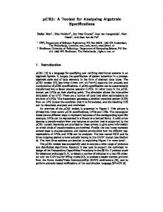
During the deployment of large European grid infrastructures, it became evident that the MPI support is lacking. In a report of the MPI Task Force of the EGEE user community [90], scientific communities “reported that only 7 sites from 26 supporting both MPI and its virtual organization ran their applications without errors”. In the course of the EU-funded project Int.EU.Grid [86] we developed mechanisms to improve the support for running MPI applications on grid infrastructures. The approach to resolving technical issues in a grid depends on its design. From our experience, grids can be organized in various ways, and one central aspect is the level of software and hardware heterogeneity in a grid infrastructure. Int.EU.Grid supported a substantial level of heterogeneity at each of its compute sites. To keep the process of booking resources and running MPI-parallel jobs transparent, it was necessary to introduce an abstraction layer into the middleware. In Int.EU.Grid, this was achieved with the help of two software components: • The CrossBroker [37], a job management service, was developed in the course of multiple grid projects, including Int.EU.Grid. • A set of modular scripts (MPI-Start) was developed for Int.EU.Grid. 17

18

CHAPTER 3. MPI SUPPORT ON A GRID Core

MPI

Scheduler

Hooks User-Defined Scripts

File Distribution

SGE

LSF

PBS

PACX-MPI

Lam/MPI

MPICH2

MPICH

Open MPI

Figure 3.1: MPI-Start architecture The CrossBroker communicates some settings to MPI-Start through environment variables; other settings can be found automatically. MPI-Start [27] was developed as a framework to support a number of heterogeneous components in a transparent way for the end user. The architecture of MPI-Start is shown in Fig. 3.1. The three core modules are job schedulers, hooks for file systems, and MPI implementations: • The supported job schedulers include Platform LSF, Torque PBS, SGE. • File systems using Network File System (NFS), and non-shared file systems, are supported. • As intra-site MPI implementations, both Open MPI and MPICH are supported. For inter-site MPI jobs, PACX-MPI is supported. For site administrators, this leads to a larger degree of freedom in the installed schedulers or MPI libraries. For the end users, this enables the transparent execution of MPI jobs. For example, in the presence of CrossBroker and MPI-Start, an end user can submit an MPI-parallel job within Int.EU.Grid sites as follows: Executable = "mpi-test"; JobType = "Parallel"; SubJobType = "openmpi"; NodeNumber = 16; StdOutput = "mpi-test.out"; StdError = "mpi-test.err"; InputSandbox = "mpi-test"; OutputSandbox = {"mpi-test.err","mpi-test.out"};

To understand how this process abstracts away technical details, we summarize how parallel job submission was done on standard EGEE sites. One option was for the user to write a set of complex and very error-prone shell scripts for running MPI applications. Alternatively, the user could manually inject MPI-Start for each parallel job. This was not necessary in the given example submission file since the CrossBroker automatically calls the installed MPI-Start package for parallel jobs. Apart from this basic functionality for running MPI applications, the support extends to more advanced concepts. As an example, the hooks framework in MPI-Start

3.2. RESOLVING LOW-LEVEL PERFORMANCE ISSUES

19

can be used to inject user-defined scripts before, during, or after execution of MPI applications on sites. These scripts enable features like application compilation, or use of advanced tools (e.g. profiling tools) to understand application performance. Other advanced concepts include cross-site execution of MPI applications; this has been enabled once again through an orchestrated effort of the CrossBroker, MPI-Start, and PACX-MPI. For more recent grid platforms like Grid’5000 [16], the overall software design is different: Grid’5000 offers less autonomy to local sites. For example, all sites universally agree on using a standardized job scheduler called OARSub, and all efforts on inter- or intra-site job reservation are part of its functionality. Other components can not be standardized, e.g. the MPI library, or the file system. In such cases, an abstraction layer like MPI-Start is still relevant and useful.

3.2

Resolving Low-Level Performance Issues

So far we have discussed a number of technical issues when using grids for MPIparallel jobs. When these issues are resolved, MPI applications can be run successfully. However, important performance issues exist with MPI applications across grid platforms. Some of these issues are quite fundamental, and are relevant both to Pointto-Point (P2P) and collective communication. From our experience, one major issue is the proper configuration of TCP and MPI settings for long-haul connections. [49] describes an important optimization on the TCP level, which applies to all MPI connections using links with high BandwidthDelay Product (BDP) (as is the case for Grid’5000). The authors introduce a reconfiguration as follows: • As administrator, increase the TCP window size. • Increase the Eager/Rendezvous threshold within the MPI library. Both of these steps are necessary for the optimization, and the idea behind is to avoid synchronization messages for as much as possible, since latency is high. The impact of the proposed optimizations for MPI and TCP can be very significant: The authors report an MPI P2P bandwidth of around 100 Mbps before, and around 950 Mbps after the optimization. In our experimental work, we made similar observations. We describe a very different approach to achieve a comparable optimization in the following section.

3.2.1

Implementing MPI P2P Communication Using Two-Phase Linear Scatter/Gather

In [2], an extension to GridFTP called “Globus Striped GridFTP” is described. Striping data segments at both ends of the network is just one of the interesting features. More importantly for us, multiple TCP streams are also tested, on a single node at each end of a network. The authors experimentally show that using multiple streams leads to increase in performance for a number of settings: Local Area Network (LAN), Metropolitan Area Network (MAN) and Wide Area Network (WAN). While the reasons behind the performance gains are not analyzed, it is noted that “up to five streams seem to make a difference in all cases, after which little additional benefit is gained”.

20

CHAPTER 3. MPI SUPPORT ON A GRID

Figure 3.2: Illustration of proposed MPI P2P implementation as linear scatter-gather across sites. For another setting, it is also noted that “parallel streams are more effective with higher Round-Trip Delay Time (RTT) and with higher packet loss”. In [29], we propose a related optimization of MPI P2P communication. We look for possible optimizations of cross-site MPI communication based on following observation: The achievable bandwidth of long-haul MPI connections was extremely low (70-80 Mbps) compared to the bandwidth provided by TCP connections, which approached 900 Mbps. These bandwidth numbers result from measurements with NetPIPE [109] using MPI and TCP, respectively. Our approach was to design an original MPI P2P implementation on top of MPI. After failing to show improvement of P2P communication by using multiple threads (a hybrid OpenMP/MPI approach), we decided to implement the same idea with MPI processes instead. At the initialization of the program, we spawn a fixed number of additional MPI processes per node. We also create a global communicator that includes all processes after this phase. Since this overhead is only at startup, it is not taken into account in our benchmarks. The original P2P communication between processes P0 and P1 is divided into two phases – a scatter phase and a gather phase (Fig. 3.2). Each phase is implemented as a linear sequence of P2P calls for the different message chunks of the original message. To exploit the parallelism of P2P calls, we cannot reuse the scatter and gather operations provided by the MPI library. The default implementation for scatter/gather is often based on the binomial tree algorithm, which transfers messages along a binomial tree. This algorithm is not suitable for exploiting a parallelization of transfer along a single link, since each link is always used once. The proposed linear scatter/gather implementation is a linear sequence of MPI P2P calls. The experiments with different combinations of P2P calls (non-blocking standard send or blocking standard or eager send) show that a sequence of non-blocking sends for phase 1 and a sequence of non-blocking receives for phase 2 perform the best. For example, if we spawn 2 additional processes at each of two nodes at the initialization, a P2P communication between process P0 on the sender node and P1 on the receiver node will proceed as follows: • P2-P5 are chosen from the global communicator to participate in this message exchange based on the host information for P0 and P1; no extra communicators need to be created. • Processes P2-P5 are notified to participate in each subsequent P2P communication. • A message of size M is fragmented into (n − 1) pieces; each helper process now

0.12

1.2

0.1

1

0.08

0.8

Time (secs)

Time (secs)


0.06 0.04 0.02

21

0.6 0.4 0.2

0

0 0

0.1 0.2 0.3 0.4 0.5 0.6 0.7 0.8 0.9 Message size (Mbytes) Point-to-point (standard) 4 added procs at both peers 8 added procs at both peers

1

0

1

2

3 4 5 6 7 Message size (Mbytes)

8

9

10

Point-to-point (standard) 4 added procs at both peers 8 added procs at both peers

(a) Message size 100 KB-1 MB.

(b) Message size 1 MB-10MB.

Figure 3.3: Comparison of non-optimized long-haul MPI P2P communication and scatter-gather based P2P communication. deals with a message of size process count.

M n−1 ,

with M being the message size, and n the new

• Processes P0-P5 call the linear scatter implementation using MPI_Isend and MPI_Recv calls; processes P0-P5 call the linear gather implementation using MPI_Irecv and MPI_Send calls. • This delays the switch point of each MPI process from the eager to the rendezvous protocol by a factor (n − 1). • At the switch point, all MPI sender processes exchange acknowledgments with the MPI receivers in parallel, i.e. the acknowledgments are pipelined in the network.

3.2.2

Experimental Results and Interpretation

The proposed scatter/gather implementation of P2P was implemented within the MPIBlib benchmarking library (Details in Ch. 6). We display the performance and pattern experiments in Fig. 3.3. If we consider the timings in Fig. 3.3a, we realize that each jump for increasing message size corresponds to a synchronization message. This is reaffirmed by the fact that the height of each jump approximately corresponds to the round-trip time. The jumps can be either caused by ACK messages during the transfer of a TCP data window, or during the MPI-specific rendezvous protocol, which asks if the receiver has issued an MPI_Recv call. There is a distinct offset in the point of jump when using 1+4 MPI processes at each end of the network instead of 1. This offset happens to be 5 times, which is not a coincidence. The jump is still of the same height, and we explain it with an acknowledgment message as explained above. But there is another important observation here – the acknowledgments of the 5 processes at each side of the long-haul connection are pipelined. If the acknowledgments were serialized, there would be no factor of improvement in the new implementation; we would only observe a shifted timing curve.

22


match(F1) matched(F1)

Sender buffer

Receiver buffer

F1

F1

match(F1)+match(F2) matched(F1)+matched(F2)

Sender buffer

F1

F2

Receiver buffer

Figure 3.4: Optimizing MPI communication across long-haul connections. Top: standard MPI point-to-point. Middle: Reconfigured MPI/TCP. Bottom: proposed optimized MPI point-to-point. Let us compare the transfer times of the original MPI implementations without modifications, the reconfigured MPI library of [49], and our version: • The original MPI implementation would have a transfer time T (M ) = α + β ∗ M + tc ∗ b

M c mc

(3.1)

In our cross-site experiments, a synch message is tc = 0.02s for each fragment mc = 128KB. This results in a much higher cost than the bandwidth-related value β. • The reconfigured MPI library would have T (M ) = α + β ∗ M . However, the receiver buffer may overflow when transferring large messages with the eager protocol. • Our modified communication has the transfer time T (M ) = α + β ∗ M + tc ∗ b

M c (n − 1) ∗ mc

(3.2)

when using a total of n MPI processes (after spawning helper processes) for the communication. The rendezvous protocol is employed, and no restrictions exist on the receiver buffer. M The term b (n−1)∗m c makes clear that the number of spawned MPI processes c (which is (n − 2)) can be limited if we know in advance the message range of the deployed MPI application. As an example, in the used test cases, if message sizes do not exceed 256 KB (which was 2 ∗ mc for the tested settings), spawning only 1


23

additional MPI processes (either at sender or receiver side) is sufficient for the best achievable speedup. In this case, we deal with fragment size of 128 KB in scatter and gather, which is the borderline of employing the rendezvous protocol. However, as we discuss in the following section, the proposed solution can also significantly help in cases of applications with unknown message ranges, and limited receiver buffers.

3.2.3

Future Work

We analyze the advantages and disadvantages of this pipelined acknowledgments solution as compared to the proposed optimal configuration at TCP/MPI level described in [49]. If the additional MPI processes are spawned only on the source and target nodes, the proposed solution adds a layer of complexity, and potentially scalability issues, to the standard MPI P2P communication, and requires spawning additional MPI processes. On the other hand, its primary advantage is that it improves performance without the need for administrator privileges or MPI reconfiguration. Significant advantages of the proposed approach can be expected in some scenarios. Let us observe the producer-consumer problem, in particular with a producer which, for a limited period, quickly produces large volumes of data, i.e. in the presence of bursty traffic. If the receiver can not match the speed of receiving and storing this data in an unexpected message queue, the eager protocol is not useful. We are forced to use the rendezvous protocol due to limitations in the receiver’s buffer. This excludes the configuration proposed by related work. But in this case a producer might produce more data than is available in its sender buffer. If we employ the proposed P2P implementation launching the additional MPI processes on different nodes, the available buffer space increases proportionally, since the aggregate memory of all nodes can be used as a larger distributed buffer until the receiver is ready to receive the data. In this sense, the proposed MPI P2P implementation can increase the tolerance for bursty traffic, and at the same time maintain high bandwidth, across links with high BDP. This is an interesting area if stream processing systems communicate via MPI, since in stream processing bursty traffic is common and buffer space is a scarce resource [3].

24


Chapter 4

A New Performance Measurement Technique Using Adaptive Communication In this chapter, we experiment with various collective communication mechanisms. This includes MPI collectives, which are an example of sender-initiated communication, but also receiver-initiated communication like the BitTorrent protocol. We show that adaptive receiver-initiated multicasts can be very efficient not only in wide-area networks, but also in non-trivial local-area networks. Based on this observation, we develop a new measurement technique for the data flow through the network, which proves efficient and reliable both in LANs and geographically distributed networks. The measurement technique builds the first phase of a two-phase reconstruction of network properties; the second phase, which is the reconstruction phase, is presented in the following chapter.

4.1

Performance of Adaptive Receiver-Initiated Multicasts

In the HPC domain, collective communication is traditionally implemented as a fixed schedule of point-to-point communications. This introduces high requirements on the selected communication schedule. In general, we have to explore a wide range of algorithms, and evaluate them based both on analytical and experimental observations [98]. These principles apply even before we have considered the network performance. There are alternatives to this difficult optimization task; instead of a fixed schedule of collective communication, there is the option of an adaptive schedule of communication. In such a schedule, messages can be delivered to the receivers in more than one route. The topic has been largely ignored in the HPC domain; yet there are indications that adaptive communication schedules can perform as good as static schedules, and are therefore a viable alternative for collective operations on a number of platforms. An important research effort in demonstrating the good performance of adaptive protocols is [23]. The author examines carefully two types of adaptive multicasting, namely sender-initiated and receiver-initiated adaptive multicasting. The sender-initiated version faces a significant number of challenges like deadlocks, duplicates, and an expo25

26

CHAPTER 4. A NEW PERFORMANCE MEASUREMENT TECHNIQUE

nential number of routes for forwarding data. Receiver-initiated multicasts solve most of these issues, and this is demonstrated in detail with two such solutions called MOB and Robber. Robber [24] is the most recent of a series of such adaptive multicast implementations. Like all its predecessors, Robber incorporates topology information in terms of intra- and inter-cluster communication in order to prevent unnecessary data transfers across wide area links. This is a major difference to topology-oblivious protocols like BitTorrent; still, Robber is the most adaptive of the presented protocols of this work. Similarly to BitTorrent, the protocol adapts to the network conditions, both on local and global level. Most of the experimental settings use highly heterogeneous networks. The emulated scenarios use links with differences in capacity in the factor of 5 to 10. Experiments confirm that Robber provides comparable performance to sender-initiated approaches, without any performance-related information through network monitoring. This is encouraging, and poses the question if the good performance of adaptive multicasts is observed also in other scenarios.

4.2

Introduction to BitTorrent

The measurement technique that we propose in this chapter is based on BitTorrent. BitTorrent [19] is a peer-to-peer protocol for the decentralized distribution of large data. One of the most popular private file sharing tools [84], recent years have seen the introduction of BitTorrent and its derivatives also as official platforms for operating system releases and the transmission of multimedia stream data (e.g., in [100]). There are compelling reasons to use BitTorrent for our purposes. The protocol is known to very well leverage a network’s capacity for file transmission [106]. Related work [33] has shown the convergence of the protocol; while protocols with faster convergence exist, the download rate of each peer converges to the upload capacity. This is demonstrated for heterogeneous peer settings, which are similar to ours. Also, the scalability of the protocol is excellent; numerous experiments [30, 59] observe linear download time O(n) with n peers even for up to thousands of nodes. This motivates the use of the proposed approach for larger and more complex settings. From the point of view of application development, BitTorrent also offers a large degree of freedom and adaptation to different scenarios. Only the messages exchanged between BitTorrent applications are clearly defined, while the protocol logic is mostly consensus and best-practice based [111, 19]. The general behavior of a BitTorrent swarm is the following. An initial uploader creates a meta information file about the content to be shared and publishes it. This file, amongst other information, contains a sub-division of the shared content into a continuous stream of small pieces. A central entity (the tracker) then distributes the IP addresses of those interested in the shared content (the leechers) and those already having it (the seeders). Leecher clients based on this information then establish individual connections with other clients and exchange information about the availability of pieces on their side of the connection. Afterwards, they decide which pieces shall be requested from which of the known remote peers. Upon the reception of a piece request, a client does not directly send over the data. Instead, peers are choked and not allowed to request or download any data until a client has decided to explicitly unchoke a peer and to inform this peer about this decision. The decision of a client to unchoke a part of the interested peers is usually based on the observed download rate. Typically, only a handful of peers per client are unchoked (including a randomly chosen peer to avoid deadlock situations – the so called

4.2. INTRODUCTION TO BITTORRENT

27

optimistic unchoking) and the choking operation is regularly repeated to reward topperforming uploaders with download slots. This tit-for-tat unchoking scheme is one of the core principles of BitTorrent. The notion of unchoking in combination with the relatively small size of the individual exchanged pieces makes BitTorrent well-suited for our cause, as it establishes both long-lived, high-bandwidth data exchanges as well as seldom-used low-bandwidth links.

4.2.1

Experimental Work in Hierarchical LANs

In [25], we extend the knowledge of adaptive dynamic protocols to study complex but less heterogeneous settings, including both the established variety of sender-initiated MPI broadcasts and a receiver-initiated broadcast (BitTorrent). We perform many experiments using not WAN settings, but LAN settings, which involve switched Ethernet clusters building a trivial or less trivial hierarchy. It is therefore interesting if in less heterogeneous settings like hierarchically switched LANs, receiver-initiated multicasts can compete with sender-initiated multicasts. We examine the performance of the fastest MPI broadcast algorithms (all of which are sender-initiated) for a hierarchical switched Ethernet network. Many studies exist for broadcast implementations in the context of Ethernet networks. The most popular broadcast implementations in MPI are flat tree, linear tree or binomial tree algorithms, and pipelined versions thereof (An introduction to MPI broadcast algorithms can be found e.g. in [123]). [97] studies in particular large message broadcasts for various Ethernet clusters, and which pipelined implementations are most efficient. For small to medium sized messages, binomial tree broadcasts or scatter/allgather implementations are common; for large messages, pipelined algorithms for broadcasts are common; studies on Ethernet switched clusters show that for sufficiently large messages, the message size, rather than the process count, dominates the runtime. Then the theoretical lower limit for a broadcast of a message is the transfer time of this message only between two nodes, since in a pipeline many nodes can overlap their message transfer to each other. The authors of [97] perform a simple analysis finding that a pipelined linear tree broadcast without contention and with good segment size comes close to the theoretical lower limit for large messages on single-switch clusters, as well as on multiswitch clusters with fully homogeneous network. The theoretical proof is trivial, and observes that on Ethernet, every node should only have one child, since a fork of multiple children is a serialization point (serial transfer to each child). The good performance of the linear tree algorithm is also experimentally confirmed for the given settings. This is indeed the default algorithm for large-message broadcasts in Open MPI; for MPICH2, the default algorithm is based on scatter/allgather. In principle, this leaves limited room for improvement: When broadcasting very large messages (Megabytes) across 10s to 100s of processes, efficient algorithms like the linear tree algorithm in MPI have a time complexity of O(M) with M being the message size. With the BitTorrent-based approach, we are not aware of a closed-form estimation of complexity, and we can only hope to reduce the complexity of senderinitiated broadcasts by a constant factor. Inspired by recent observations on sender- and receiver-initiated multicasts, and some knowledge gaps summarized in Table 4.1, we here build a bridge between the algorithms used in the high-performance computing domain and the algorithms used in the distributed computing domain for large message broadcasts. In particular, we examine if both sender- and receiver-initiated multicasts have their justification when using homogeneous or less homogeneous hierarchical networks.

28

CHAPTER 4. A NEW PERFORMANCE MEASUREMENT TECHNIQUE Underlying network Very homogeneous Very heterogeneous Some level of heterogeneity

Optimal broadcast algorithm Linear tree algorithm (static) topology-aware pipelined trees (static) or receiver-initiated multicasts (dynamic) Unknown

Table 4.1: Optimal large-message broadcast algorithms for the two extremes of homogeneous or heterogeneous networks according to recent research

4.2.2

Experimental Setup

The network for our experimental setup is a hierarchy of Ethernet clusters (details are provided in in Sect. 5.4). The used setting has significantly less heterogeneous network properties than settings usually used in the distributed computing domain, but we do not consider this a disadvantage. On the contrary, this moderately heterogeneous setting is more typical for high-performance computing. The original Python-based BitTorrent client by Bram Cohen is used, with following minor modifications: • File I/O was removed. Instead, dummy data strings are generated on-the-fly and transferred over the network. • The wall clock time is taken at initiation of the class StorageWrapper and at download completion in the same class. The time difference is used as reference. For discovering the runtime algorithm and fragment size for pipelining in Open MPI we used PERUSE [68]. The decision making process in Open MPI is very complex and runtime checks with PERUSE are a reliable way to find which algorithm is used for particular process number and message size. For MPICH2, we use related work and the source code to find which algorithm is being used.

4.2.3

Timing Mechanism Used in BitTorrent and MPI

In this section, we give a detailed explanation of the timing methodology used consistently both in BitTorrent and MPI experiments. This is important since BitTorrent originally does not provide such timing, while MPI supports timing calls and logical operations with the collective call MPI Reduce. The runtime setup for BitTorrent involves starting a BitTorrent tracker and then launching BitTorrent clients simultaneously identically to MPI program startup. The execution time of a BitTorrent program is then taken as the wall clock time between the start of a StorageWrapper instance and the moment download completion is registered. A BitTorrent client then has to be explicitly terminated since it has no concept of completing a collective communication. In MPI, a barrier call is made, and then the wall clock time is taken before and after the broadcast operation. Then, timing mechanism is as follows: • In each run and for both types of broadcasts, 64 processes are run, and each of them provides a different wall clock time to finish. As a reference, we take the maximum time between all processes both for BitTorrent and MPI. • We also perform a number of iterations for each run. As a reference, we take the average of all iterations - again, both for BitTorrent and MPI.

4.2. INTRODUCTION TO BITTORRENT 30

30

MPICH2 64 procs broadcast Open MPI 64 procs broadcast BitTorrent 64 procs broadcast

25


25

20

Runtime (secs)

Runtime (secs)

29

15

10

5

20

15

10

5

0

0 1

10

100

1000

1

Message size (MB)

(a) Using single cluster Bordereau.

10

100

1000

Message size (MB)

(b) Using clusters Bordereau and Borderline.

Figure 4.1: 64 node broadcasts without the main bottleneck link. On this homogeneous setting, the linear tree algorithm performs best as expected for very large messages, but BitTorrent also performs well. For each message size and each setting, we perform 5 iterations for MPI and BitTorrent.

4.2.4

Benchmarks on a Homogeneous Setting

In the first setting, we test the performance of the presented broadcast algorithms without involving the main bottleneck link. We first use 64 nodes on the Ethernet cluster Bordereau (Fig. 4.1a). Then we use 55 nodes on Bordereau and 9 nodes on Borderline (Fig. 4.1b). We benchmark three broadcast versions - MPICH2, Open MPI and BitTorrent. The used message sizes are 1, 5, 10, 50, 100 and 239 MB. The results for both runs are similar. They demonstrate that for the message sizes 5 MB and 10 MB, MPICH2 marginally outperforms Open MPI, but Open MPI and the linear tree algorithm is most efficient for the rest of message sizes. However, the broadcasts with BitTorrent come very close to the Open MPI broadcasts and even outperform MPICH2 for large messages. This result is unexpected, since the initial assumption is that BitTorrent-based broadcasts are not suitable for homogeneous clusters – however, BitTorrent performs excellent for both settings. The difference to the linear tree broadcast is even minimal for the second run. We interpret this with the fact that this run involves the Nortel-HP link as well and this introduces an increase in network heterogeneity.

4.2.5

Benchmarks on More Heterogeneous Settings

In the second setting, we involve the main bottleneck link in two different runs. First, we use 32 Bordeplage nodes and 32 Bordereau nodes (Fig. 4.2a). Then, we involve 32 Bordeplage nodes, 25 Bordereau nodes and 7 Borderline nodes (Fig. 4.2b). For the MPI runs, processes are started in the way they are listed. We consider this the most efficient process-to-node assignment for the linear tree algorithm. Inter-cluster communication is minimized, and intra-cluster communication has been proved to be efficient anyway. For MPICH2, there is no simple solution for providing an optimal file for the scatter/allgather algorithm, and we provide the same process-to-node mapping. We use the same broadcast implementations and message sizes as before. The benchmarks show that on both settings, for message sizes of 50 MB and larger BitTorrent

30

CHAPTER 4. A NEW PERFORMANCE MEASUREMENT TECHNIQUE 35

40


30

30 Runtime (secs)

25 Runtime (secs)


35

20 15 10

25 20 15 10

5

5

0

0 1

10

100

1000

Message size (MB)

(a) Clusters Bordeplage and Bordereau.

1

10

100

1000

Message size (MB)

(b) Clusters Bordeplage, Bordereau and Borderline.

Figure 4.2: 64 node broadcasts with main bottleneck link. This setting has some level of heterogeneity, and BitTorrent performs better than MPI for large messages. (which is oblivious of the topology) outperforms both MPICH2 and Open MPI. A secondary result is that for the same large message range, the scatter-allgather algorithm used by MPICH2 outperforms the linear tree algorithm used by Open MPI.

4.2.6

Interpreting the Results

The performance of the linear tree algorithm of Open MPI decreases significantly with the introduction of a bottleneck link; the throughput decreases by around 50 %. On the other hand, the binomial tree and particularly the BitTorrent algorithm perform excellent. The total amount of received data at all processes does not differ between the different broadcast algorithms. However, the schedule of point-to-point communication differs between the three algorithms. The MPI tree-based algorithms are fixed, and data flows in one direction – e.g. the linear tree algorithm only transfers the exact message size once across the bottleneck link. On the other hand, BitTorrent can use a larger number of parallel point-to-point connections to dynamically schedule the broadcast. This allows the protocol to utilize the network better. A more detailed analysis confirms that data is broadcast in different ways for BitTorrent and MPI. In Fig. 4.3, we display a ”profile“ of a 239 MB broadcast with Open MPI and BitTorrent. The dynamics of data movement in a broadcast is difficult to visualize. We choose a view representing the amount of data passing through all switches in any direction during the broadcast. For this purpose we do not use monitoring on the switch level, but a different approach depending on the library we use. For MPI, we know the underlying broadcast algorithm (linear tree) and placement of processes, and we can determine the data movement a-priori. For BitTorrent, as explained in this work, this is not possible, so we measure traffic through additional profiling at each peer instead. Fig. 4.3 displays the BitTorrent switch traffic in blue, and the MPI switch traffic in green. It reveals that inter-cluster communication is more intense with BitTorrent than with MPI – a typical 239 MB broadcast with the setting of Fig. 4.2b transfers around 3,4 GB across the bottleneck switch (in any direction) with BitTorrent, and only the minimal 239 MB with Open MPI. Within clusters however, data exchange with BitTorrent is less intense than with the linear tree algorithm. This behavior can be partially explained with the fact that BitTorrent is topology-unaware. However, the protocol observes topology to some extent, since the intra-cluster communication is still more intense than intercluster communication. Fig. 4.3 suggests that rather than ignore topology, BitTorrent

4.3. BANDWIDTH MEASUREMENT TECHNIQUES: RELATED WORK

Bordeplage

3,87GB 5,59GB

Borderline

BitTorrent MPI

31

2,8 GB 5,34GB 7,22GB

3,4GB 239MB

1,96GB 239MB

319MB 1,4GB

Bordereau

614MB 239MB

Figure 4.3: Data flow in a 239 MB broadcast with BitTorrent and MPI on three Bordeaux clusters. BitTorrent transfers are adaptive and follow a different ratio and direction from the fixed MPI schedule. uses a different ratio between intra- and inter-cluster communication. We conclude that in the presence of bottleneck links, BitTorrent dynamically finds a more efficient schedule for a broadcast than a good tree-based algorithm. As an interesting direction for future work, this schedule could possibly be used as input to sender-initiated multicast algorithms. For example, the more intense data transfer through the bottleneck link seems to improve, rather than reduce performance for BitTorrent. Therefore, the use of multiple spanning trees in parallel in the MPI library could be explored.

4.3

Bandwidth Measurement Techniques: Related Work

There are good introductions to bandwidth and capacity estimation methods [101, 23]. Among others, they include important definitions on properties like capacity, available bandwidth, and Bulk Transfer Capacity (BTC), and describe methods to measure them. These are fundamental and important properties in computer networks; however, they do not describe the throughput of applications; rather, network properties are measured under some strong assumptions. We do not strive for completeness here, and only mention a few examples to illustrate the different goals and assumptions made by network-centric approaches. One technique called packet pair technique [17] efficiently measures link capacity; however, a common assumption when measuring capacity is the absence of cross traffic when probing the network. A more recent technique called packet tailgating [74] also measures link bandwidth; however, if there are more than a few hops between sender and receiver, the technique is inaccurate. We do not wish to make assumptions on the network, and follow an approach which is not concerned with a generic network model under ideal conditions; instead, we are focusing on measuring the bandwidth achieved by end applications. This can include cross traffic and hardware or software failures. Our measurement tools are either benchmarking suites, or applications like peer-to-peer clients [30, 31]. We are measuring network properties from an application-centric perspective, mostly interested in

32


achievable bandwidth or throughput, and use these terms in agreement with related work like [23].

4.3.1

Exhaustive Bandwidth Measurements

NetPIPE [109] is among the most popular tools for measuring the maximum bandwidth along a link. The design of NetPIPE is ”motivated by the need to assess the performance of communication bound applications“. The tool is protocol independent; it attempts to find the saturation point after which no increase in throughput is observed. The nature of such benchmarks is quite exhaustive. Another tool employing similarly costly measurements, but with the option of using multiple parallel streams, is iperf [119]. These tools measure the throughput along a link. For measuring the throughput for entire networks, it is possible to measure the maximum bandwidth step by step for each link. However, this approach will not account for links sharing a bottleneck link. To also be able to identify bottleneck links, similar measurement procedures can be employed, but using multiple links or paths in parallel. Two essential steps are generally involved when trying to identify both maximum bandwidth and bottleneck links: • In the first step, an intense communication is established along a path until its capacity is reached. • In subsequent steps, in addition to the first step, an intense communication is established along another path, until its capacity is reached; the capacity of the previous path is reexamined. If no change in bandwidth is observed, then the links are probably independent – more pairs communicating in parallel could unveil a bottleneck at a later point. But if the bandwidth of the node pairs under examination decreases, then it is clear that they share the same physical (and logical) link. Following this procedure, experiments are performed until the entire network is reconstructed. While intuitive, this approach is very expensive. The measurement procedures have polynomial complexity, even after some optimizations using heuristics or parallelism. Related work [11, 80] following these techniques to reconstruct large topologies belongs to the area of network tomography. While [80] infers a qualitative view of the network, [11] infers a more quantitative view, including labeling of actual achievable bandwidth. The most time-consuming phase in these approaches is the bandwidth measurement.

4.3.2

Measuring Achievable Bandwidth Based on Dynamic Parallel Access

Our measurements differ from the above techniques. Early work [106] uses the term ”dynamic parallel access“ and experimentally verifies that a client using a number of parallel TCP connections to different servers will download a file with a rate approaching the upload rate of the fastest server. When using a number of parallel connections, more data will be naturally transferred through the links with higher bandwidth. Indeed, the BitTorrent protocol, which will be introduced in detail shortly, uses a number of parallel connections to exploit this network feature.

4.4. FORMAL DEFINITION OF PROPOSED MEASUREMENT

33

Few efforts have explored the use of dynamic parallel access and BitTorrent for network measurements. A notable example is BitProbes [58], which layers a set of instrumented BitTorrent clients (an overlay swarm) on top of existing BitTorrent swarms. These clients are guaranteed to participate with the rest of the peers due to the optimistic unchoking in the tit-for-tat strategy. To infer capacity, the clients of the overlay swarm record the arrival times of packets. These arrival times serve as input to a capacity measurement tool called MultiQ [66]. The tool requires ”a significant number of packets“ to reliably estimate a path capacity; the measurement period in BitProbes is 1 week. The authors claim that BitProbes provides sufficient input to MultiQ for reliable capacity estimation.

4.4

Formal Definition of Proposed Measurement

In general, the BitTorrent protocol distributes data without requiring the availability of all peers. In contrast to this common scenario, we use fully synchronized instrumented execution of BitTorrent clients until all clients have downloaded a file, which we naturally call BitTorrent broadcasts. The used metric in all reconstruction methods is derived from these broadcasts and is bandwidth-related. We observe the communiM cation network as a directed graph G = (V,E). A file of size M is distributed as 16KB fragments of 16KB to all nodes v ∈ V using BitTorrent broadcasts (The actual fragment size is irrelevant for the metric – the 16 KB are simply the observed fragment size when using the original BitTorrent client). If v1 →i v2 denotes the number of fragments sent directly from v1 to v2 within broadcast operation i, then we define the metric w per edge e for one run as w(e) = v1 →1 v2 + v2 →1 v1

(4.1)

with e = (v1 , v2 ). Since performing more iterations significantly increases the accuracy of the metric, for n iterations we simply aggregate the individual runs into Pn v1 → i v2 + v2 → i v1 wn (e) = i=1 (4.2) n with e = (v1 , v2 ). We have instrumented the original Python version of the BitTorrent client written by Bram Cohen and available in most Linux distributions. We introduce simple and efficient profiling of the arriving data as follows: At the reception of each data fragment, a counter is incremented associated with the sending peer using a hash table of counters. At the end of a run, all peers have a record of the source peers and the number of fragments they received from each peer. As an example, in a broadcast operation involving 64 nodes on two clusters on one geographical site, we display measurements for a randomly chosen node in Fig. 4.4. The bars represent the metric as defined above for 36 iterations for all edges which include the fixed node. Since the results involve many iterations, the chosen node exchanges fragments with all 63 peers. For clarity, we have grouped on the left side the metric values for the 31 peers in the local cluster, and grouped the values for the 32 remote nodes on the right side. While we see a high level of noise, it is also evident that the metric converges to levels correlated to the achievable bandwidth. The higher bars roughly correspond to the edges to local nodes, and the lower bars – to edges to remote nodes.

34

CHAPTER 4. A NEW PERFORMANCE MEASUREMENT TECHNIQUE 1400

Exchanged fragments (averaged over 36 iterations)

1200 1000 800 600 400 200 0 Peers from local cluster

Peers from remote clusters

Figure 4.4: w36 (e) as measured for all edges e to a randomly fixed node (36 iterations). On the left are edges to local cluster nodes, on the right are edges to remote nodes.

4.5

Efficiency of the Metric

The main strength of our method is that it takes only a single broadcast of a large message per run to collect data on a large subset of all possible peer-to-peer connections. In our setup, the observed complexity of BitTorrent broadcasts is O(M) – linear in the message size M. We verified experimentally that as we alter the number of nodes, the BitTorrent broadcast requires nearly constant time. According to practices from highperformance computing, our reference time for the completion of a BitTorrent broadcast is the maximum download completion time of all the BitTorrent clients, which we start synchronously. For 32, 64 and 128 nodes, the broadcast of a large message (here: 239 MB) always takes about 20 seconds on the Grid’5000 infrastructure, even when the nodes are spread across 4 geographically distributed sites. Related work [59] also suggests that a high download rate can be sustained for very large peer numbers; the number of participating peers in such experiments typically does not alter the estimated time of O(M) for all peers to download the file. Other work [129] also demonstrates that the BitTorrent protocol is competitive with client/server architectures in its peak download rate. Each step in the algorithms of related work is very time consuming. First, every link has to be saturated until the maximum bandwidth on that link is reached. This is a costly operation which incurs heavy network overhead. The second challenge consists of probing the link bandwidth in parallel for multiple links. This process is repeated until all nodes have been sufficiently tested. For example, [11] performs such tests only with at most triplets of nodes. It is stated that triplets are sufficient as long as the single-link experiments can reach the maximum capacity. Even with this assumption, all possible triplets need to be tested in the worst case. This step is performed since it is assumed that there is no a priori knowledge of the topology of the network. The observed complexity of the algorithm in this case is O(N 3 ), where N is the number of nodes. The algorithm proposed by [80], on the other hand, tests pairs incrementally, fully in parallel and without limiting the maximum number of tested links at a time. In specific cases, where no interference of links is observed, the complexity is estimated

15 5 0

Frequency

4.6. LEVEL OF RANDOMNESS WITH SINGLE RUNS USING THE METRIC 35

0

1000

2000

3000

4000

5000

6000

Exchanged fragments between peers

Figure 4.5: Distribution of measured metric w(e) for a fixed edge e and 36 independent iterations. at O(N 2 ). The only empirical experiments performed are for networks of 20 nodes, and these take about one hour to complete. This complexity makes it infeasible to perform such bandwidth-related network tomography on large-scale computer networks. Related work details this issue and resorts to running simulations.

4.6

Level of Randomness With Single Runs Using the Metric

If we examine the volume of exchanged data shown in Fig. 4.4 over a number of iterations, we notice that a total of 22533 fragments are exchanged with local cluster nodes, and 6337 fragments are exchanged with remote nodes. This is a clear indication that with BitTorrent broadcasts, data flows with a preference for high bandwidth links. Furthermore, we observe this phenomenon quite reliably in our experimental data. We have previously defined a single run of our metric as transmitting a single file which takes approximately 20 seconds. As the operation of the BitTorrent protocol is stochastic, and the data transferred across each link varies from run to run, it is important to attempt to characterize the accuracy of the metric we have defined for a single run. Thus, we now observe how the metric fluctuates using one Grid’5000 site (Bordeaux). We focus on an edge between 2 nodes randomly chosen from within a cluster. Each run measures the metric w(e) independently (no aggregation is used). Fig. 4.5 shows the distribution of w(e) along the fixed edge over 36 runs. In 13 of the 36 runs, the two peers do not exchange any data with each other. In the other 23 runs, the exchanged data varies between 3 and 6304 fragments. This distribution shows that the variance is very high. For comparison, when running the well known NetPIPE tool [109] to establish the maximum achievable bandwidth along the link between two peer nodes on the same compute cluster used above, the variance is very low and the distribution is dense around 890 Mbps. Fig. 4.5 suggests that while inexpensive to compute, the metric is very variable for single runs. With this level of measurement noise and randomness, a good analysis technique will be needed to extract meaningful data from these measurements.Yet one important consideration is that our analysis method does not consider each link’s bandwidth in isolation, as is the case for more quantitative methods looking for achievable bandwidth, and this to some extent is a relaxation on the part of measurements. We briefly list the BitTorrent properties which are responsible for the variance and

36


high degree of randomness between single runs of the metric: • Initially, BitTorrent clients randomly choose their initial peers (adjustments in the peer selection are part of the protocol for longer runs). • By default, BitTorrent internally limits the number of parallel uploads to 5, and this indirectly limits the number of parallel downloads. • Another protocol feature is that the number of total peers to store is by default limited to 35. This means that for larger numbers of nodes and a single broadcast, measurements using this protocol will not provide a complete graph - only a subset of possible connections will be measured. One solution to this problem is to aggregate the measurements over a number of BitTorrent broadcasts, as we shall see. • Using a BitTorrent broadcast operation means that nodes which are better connected to the ‘root node’ are more likely to receive more fragments from the root. This is simply due to the asymmetric way data flows in a broadcast operation as compared to, for example, an all-to-all transmission. However, in our experiments this was never an issue during the reconstruction and analysis of our networks. If this affects results in some cases, a simple solution is using different root nodes over a number of runs. These are characteristics of the protocol, which, while important for transmission efficiency and reliability, increase the variance of our measurements, and could make the reconstruction process hard. Iteration significantly improves the quality of the metric.

4.7

Iteration of BitTorrent Broadcasts and Convergence

While a single broadcast measurement has a high level of noise and randomness, aggregating data over a number of iterations resolves these issues. The BitTorrent protocol converges to download rates reflecting the upload capacity of links; this has been demonstrated in [33]. In our experiments, we assume that the upload/download capacity of links is identical. This means that for the metric w(e) we expect: wn (e1 ) bw(e1 ) ∀e1 , e2 : w → bw(e for n → ∞. n (e2 ) 2) In order to quantify the number of iterations needed to sufficiently improve accuracy, the key questions are: • How close is the single run data to an “ideal” representation of the peer-to-peer bandwidth when performing bulk data transfers? • How fast does the aggregated data over a number of runs converge to the “ideal” representation? These questions could be addressed by an analytical approach, which quantifies the deviation of the proposed metric from an exact solution. However, we follow a more holistic approach: Instead of an isolated analysis of the measurement procedure, we use its output as input to reconstruction techniques, which are presented in Ch. 5. The accuracy of the measurements is then evaluated based on the outcome of the reconstruction techniques.

NMI

4.8. FURTHER ISSUES WITH BITTORRENT AND EXPERIMENTAL SETUP 37 1.2 1 0.8 0.6 0.4 0.2 0

60-Second unchoke interval 5-Second unchoke interval

1

2

3

4 Iterations

5

6

7

Figure 4.6: A shorter choke/unchoke period negatively impacts the quality of our method. This is an indication that the tit-for-tat strategy should be removed from peerto-peer protocols for efficient bandwidth measurements. The accuracy is measured with Normalized Mutual Information (NMI) along the y-axis. This measure compares the results of a reconstructed clustering to the (accurate) ground truth clustering. In other words, we address the question of accuracy in an end-to-end manner, by quantitatively evaluating the performance of the entire system which uses these measurements.

4.8

Further Issues with BitTorrent and Experimental Setup

We already presented a number of issues with the noise and randomness intrinsic to BitTorrent. In this section, we present some further issues. On the one hand, we find that the tit-for-tat strategy of the BitTorrent protocol to some extent obstructs the proposed measurements. On the other hand, we discuss an alternative experimental setup with passive and non-controlled mechanisms for measuring bandwidth, which would allow an easier deployment on a large scale.

4.8.1

Tit-for-Tat Strategy

One important implication of the tit-for-tat policy, which plays an important role with the longer running simulated BitTorrent downloads, is that clients become more adaptive. Towards the end of each run, faster uploaders are preferred. In experimental work with a simulator, we found that this adaptiveness obstructs the accuracy of the measurement procedures. We performed simulated tomography with a complex network (network N2 of Ch. 5). We compared how BitTorrent clients perform with 5-second vs 60-seconds choke/unchoke period (One run completes within 5 minutes of simulated runtime). We expect the tit-for-tat policy to manifest itself better in the shorter 5-second choke/unchoke period. For this policy, the accuracy of the simulated tomography method is significantly lower in the first few iterations (Fig. 4.6). Our interpretation is that a more adaptive client does not provide a broad enough metric w to various peers, since it prefers faster ones; as a consequence, it can produce less reliable results. This is significant: The tit-for-tat strategy is at the core of BitTorrent protocol, but some of its aspects like the tit-for-tat policy should be redesigned if possible for the purposes of our measurements.

38


4.8.2

Number of Active Connections

Another aspect which can influence the measurement procedures is the number of simultaneously active connections. There is a fine balance between keeping too few and too many active connections. Having few connections results in a less dense graph per BitTorrent measurement, and potentially larger number of iterations before convergence. However, having too many active connections can lead to congestion and TCP-specific congestion control. The BitTorrent specification is rather generic, stating that an algorithm “should cap the number of simultaneous uploads for good TCP performance”. The default number of active peer connections is set to 5.

4.8.3

Shortcomings of Proposed Setup

In its current design, the proposed measurement belongs to the active network tomography area; it assumes that all BitTorrent clients are part of a controlled environment. They are instrumented, and can be started and stopped at will, which requires minor modification of the clients, and administrator privileges at the nodes participating in the measurements. Most real-life environments do not offer such level of control. Furthermore, due to the controlled execution entirely for the purpose of traffic measurements, dummy data is transferred. While these measurements are efficient, they are quite unusual compared to the common scenario in a swarm. In real-life scenarios, the swarm distributes useful data, and clients can join and leave at any time without any control mechanism. Therefore, the BitTorrent protocol seems much more suitable for a different measurement setup. We see two possible approaches to passive measurements with BitTorrent in real large-scale settings, and present them in Fig. 4.7. One possibility is the introduction of an overlay swarm of instrumented clients as described in [58]. This has advantages for the proposed measurements: it allows for more extensive measurement modifications or changes in protocol to be introduced into the overlay swarm without affecting the non-instrumented peers in any way. The main disadvantage is in the performance loss. Optimistic unchoking is the main mechanism of involving the overlay swarm into the overall data exchange, and this only can happen gradually. An efficient measurement procedure is unlikely in such a scenario. An alternative to this approach, which is likely to be much faster in gathering measurement data, is to instrument the entire swarm of BitTorrent peers. Then, a measurement log can be taken at any time with a high degree of accuracy. Technically, this is possible without any overhead, or loss of anonymity for the peers; some authors [82] argue that in practice an instrumented BitTorrent client is unlikely to be adopted by a large user community.

1

2

3

4

M

ea s

O sw ver ar lay m

ur em

en t

4.8. FURTHER ISSUES WITH BITTORRENT AND EXPERIMENTAL SETUP 39

5

6

7

8

9

10

M

ea su

re m

en t

(a) Launch overlay swarm, wait until all peers are involved in data exchange, take measurement.

1

2

3

4

5

6

7

8

9

10

(b) The swarm is instrumented, take measurement at any time.

Figure 4.7: Two approaches to passive BitTorrent measurements. (a) Introduction of an overlay swarm. (b) A fully instrumented swarm.

40


Chapter 5

Performance-Based Reconstruction of Networks The presented measurement technique in previous chapter provides raw bandwidth data, which in principle can provide input to performance-aware collective communication. In search for ways to transform the performance data into more meaningful representations, we first introduce some useful tools for tracing, analyzing and visualizing measurement data. We then focus on topology, and design two topology generation methods. One method is based on a clustering method called modularity-based clustering. We first successfully apply it for recognizing bandwidth clusters. Then we proceed to develop a hierarchical clustering algorithm, which generates a bandwidth-based hierarchy. The hierarchy can be seen as another representation of topology. Another method is based on the classical spanning tree algorithm for graphs, and generates a topology as a tree.

5.1

Useful Tools for Visualization and Analysis

In this section, we present some of the tools we used in our work. First we introduce the Paraver toolkit, which we extend to trace and visualize socket communication with BitTorrent. Then we introduce Graphviz, which gives us important hints about the suitability of modularity clustering methods.

5.1.1

Tracing BitTorrent Communication Using the Paraver Toolkit

The metric w provides a count of the exchanged data fragments between peers. We described how to collect this metric – we introduce counters to the BitTorrent clients. In effect, this type of measurement is a profiling technique. One of the main advantages of profiling is that it does not introduce a great overhead to the profiled application. Its main disadvantage is that sometimes profiling is not sufficient for detailed analysis. When it comes to performance measurements, the main alternative to profiling is tracing. Tracing provides great detail for analysis, since it allows to timestamp each event of interest during execution. This means that execution can be analyzed with runtime in mind, and with an understanding of the corresponding dynamics of the application during execution.

41

42

CHAPTER 5. RECONSTRUCTION OF NETWORKS

Usually, an application is being traced, the traces are then visualized and analyzed, performance bottlenecks are identified, and the application is modified. This is an iterative process, which is continued until the performance of the application is satisfactory. Our scenario for tracing, however, is rather different. Instead of analyzing an application, we wish to perform measurements as proposed in Ch. 4, and design efficient performance-aware collective communication. This unusual scenario, in which the underlying communication library rather than the application is being analyzed, is sometimes referred to as introspective performance analysis. There is related work in the HPC community; some efforts instrument events within the Open MPI library [68, 67], and use the Paraver toolkit to extend their knowledge beyond the application level and into the MPI communication middleware. The Paraver toolkit [61] belongs to the most popular tools for tracing, visualizing and analyzing applications. Some of the supported programming interfaces include MPI, OpenMP, POSIX Threads (Pthreads), OmpSs and Compute Unified Device Architecture (CUDA), but user-defined events enable any types of events to be traced. Some of our goals in tracing BitTorrent communication are: • to provide automatic and more flexible mechanisms to gather and process the measurement metric w. • to provide a visualization for the dynamics of data traffic during communication between peers. • to generally have a powerful visualization and analysis tool at hand for BitTorrent communication. We used the original Python client written by Bram Cohen [19]. The instrumentation with Paraver was achieved with following steps: • Trace calls from the user API were added to all socket communication calls. • Some calls were “borrowed” from the MPI library. This included initialization and finalization of the tracing component of Paraver called Extrae (through MPI calls intercepted by Extrae), as well as a barrier call for a synchronized termination of the clients. We demonstrate some of the new capabilities of this approach by tracing a small 10 MB BitTorrent broadcast. As experimental setting, 32 nodes are run on the site Bordeaux, 16 on the Bordeplage cluster, and 16 on the Bordereau cluster (see Sect. 5.4 for details). The received or sent bytes from/to each peer can immediately be visualized, and an additive view of both 1 would represent a measure equivalent to the measurement metric w we introduced earlier. Fig. 5.1 visualizes such a histogram which shows in a matrix how much data is received by a peer from each other peer, varying from 0 to nearly 4 MB per peer. This view shows how data can be distributed with dynamic and adaptive receiver-initiated protocols. It can be observed that there is no symmetry in the data exchange between clusters. For example, the top-right half of the plot shows that little data is received from Bordeplage by Bordereau. The bottomright half shows that much more data is received from local Bordereau nodes. Since data exchange is adaptive, this can hint at issues of inter-cluster communication. 1 Such

a view is not currently available in Paraver.

5.1. USEFUL TOOLS FOR VISUALIZATION AND ANALYSIS

43

Figure 5.1: A histogram showing the received data in a 10 MB broadcast between 32 BitTorrent peers. The x axis stands for peers 1 to 32, and the y axis for peers 1 to 32 with count starting from the top. For clarity we encode the received data in a colour scheme. Bright yellow is the minimum of received data (here: 0 bytes), dark blue is the maximum received data (here: 3,7 MB) from a single peer, and linear gradients are used in between. Peer 0 (leftmost column) is the seeder, so it does not receive data. Every other peer receives varying amounts of data from its peers. For such a metric, however, we could have also used profiling rather than tracing. To demonstrate the capabilities of tracing, we choose to display as an example the “messages in transit” at each peer during the same experiment described above. The messages in transit are messages being sent, or being received, where the point-topoint communication is not complete yet. Fig. 5.2 shows a runtime with this metric. A careful observation shows that the Bordeplage nodes (upper 16 timelines) have many messages in transit for longer periods than the Bordereau nodes (bottom 16 timelines). This could be an indication of a slower network on Bordeplage than on Bordereau. Based on such observation, we can see hints for possible performance-based models using the Paraver toolkit in conjunction with BitTorrent clients. It is likely that more intuitive and meaningful views can be generated, depending on the interest of the developer. Further methods are the subject of future work. However, it should be noted that powerful performance tools like Paraver offer possibilities, but no answers; ultimately, the application or middleware developer is responsible for designing meaningful views to detect issues, and to find solutions.

5.1.2

Cluster Visualization with GraphViz

In order to investigate the potential for an algorithmic clustering method to deduce the ground truth clusters from the measured network, we first visualize the measured network data using a network layout algorithm. On each layout visualization, we use nodes of different shapes to represent different ground truth clusters. (The exact details of how the ground truth is produced from the physical network topology will be discussed in Section 5.4). As is shown visually in Figures 5.3, 5.4, 5.5, 5.6 and 5.7, the application of a layout algorithm to the measured networks allows us to visually observe groups of nodes the layout places close to each other. These groups clearly correspond to the ‘ground truth’ logical clusters of the underlying computer network. For these visualizations, we layout the networks using the implementation of the Kamada-Kawai spring weighted graph layout algorithm [62] from the ‘Graphviz’ software package [34], in which we make the length of edges between nodes inversely

44


Figure 5.2: A timeline (x axis) of messages in transit for a 10 MB broadcast between 32 BitTorrent peers (y axis). For clarity we use a colour scheme. Green is the minimum messages in transit (here: 0), orange is the maximum messages in transit (here: 18), and linear gradients are used in between. This view shows the dynamics of data distribution during runtime. The nodes on Bordeplage (top 16) have many messages in transit for longer than the nodes on Bordereau (bottom 16).

172.16.0.46

172.16.0.45

172.16.0.48

172.16.0.33

172.16.0.43

172.16.0.41 172.16.0.49

172.16.0.4

172.16.0.8

172.16.0.42

172.16.0.36

172.16.0.6

172.16.0.32

172.16.0.9

172.16.0.50

172.16.0.3

172.16.1.77

172.16.0.39

172.16.0.40

172.16.0.7

172.16.0.5

172.16.0.35 172.16.0.37

172.16.0.29 172.16.0.38

172.16.1.93

172.16.0.30

172.16.0.24

172.16.0.34

172.16.0.23

172.16.0.26

172.16.1.71

172.16.0.25

172.16.1.69

172.16.0.27

172.16.2.4 172.16.0.28

172.16.1.7

172.16.1.86

172.16.1.91

172.16.1.85

172.16.1.70 172.16.1.72

172.16.1.9

172.16.1.90

172.16.1.74

172.16.1.87

172.16.1.84

172.16.1.8 172.16.1.83

172.16.2.6

172.16.1.68

172.16.2.8

172.16.2.9 172.16.1.76 172.16.1.81

172.16.1.82

172.16.1.92 172.16.1.89 172.16.1.78

172.16.2.7

172.16.1.75

172.16.1.73

172.16.1.80

Figure 5.3: Applying Kamada-Kawai layout (using the Graphviz’ ‘Neato’ tool) to the weighted graph of experiments using Bordeaux site. The configuration has 64 nodes, divided between 3 physical compute clusters. These 3 physical compute clusters give rise to only 2 logical network clusters, as there is a fast link between the ‘Bordereau’ and ‘Borderline’ physical clusters. The shape and color of each node rendered reflects the labeling of the ground truth cluster it is in. We render only the edges in the top half of all edges, by weight. While the graph is too dense to visually make out any structure due to edge weight, it is clear that the layout algorithm is grouping nodes corresponding to their ground truth. This provides grounds for expecting a graph clustering algorithm to find these clusters.

5.1. USEFUL TOOLS FOR VISUALIZATION AND ANALYSIS

45

172.16.113.3

172.16.113.50

172.16.113.18

172.16.113.126 172.16.113.135

172.16.113.117

172.16.113.16

172.16.113.139

172.16.113.38

172.16.113.19

172.16.113.26

172.16.113.123

172.16.113.124 172.16.113.49

172.16.113.56 172.16.113.36

172.16.113.92 172.16.113.76

172.16.113.140

172.16.113.33

172.16.113.51

172.16.113.133

172.16.113.95

172.16.113.35 172.16.113.28

172.16.113.98

172.16.1.12 172.16.1.10

172.16.113.134

172.16.113.9

172.16.113.136

172.16.113.138

172.16.113.52

172.16.113.57

172.16.2.9 172.16.0.6

172.16.2.7

172.16.0.51 172.16.0.5

172.16.0.9

172.16.2.3

172.16.0.50

172.16.2.4

172.16.0.34

172.16.0.28 172.16.0.49

172.16.2.1 172.16.0.42

172.16.1.11

172.16.0.47

172.16.0.4

172.16.0.46 172.16.0.3

172.16.0.37

172.16.0.32

172.16.0.33

172.16.0.36

172.16.0.35 172.16.0.44

172.16.0.48

172.16.0.8

172.16.0.39 172.16.0.30

Figure 5.4: Applying Kamada-Kawai layout to weighted graph of experiments using 64 nodes on Bordeaux and Toulouse sites, and the same rendering options as for Figure 5.3. Toulouse is represented here by diamonds; the ground truth clusters represented by circles and triangles both belong to Bordeaux. Our non-hierarchical clustering method does not recover this ground truth; it finds only two clusters, one for Toulouse and one for Bordeaux. The third ground truth cluster is distinct in the visualization, however, showing that the BitTorrent measurements do reflect it.

172.16.113.38

172.16.113.35

172.16.113.140

172.16.113.133

172.16.113.33

172.16.113.28

172.16.113.19 172.16.113.126

172.16.113.3

172.16.113.139

172.16.113.134

172.16.113.136

172.16.113.95

172.16.113.26

172.16.113.123

172.16.113.135

172.16.113.36

172.16.113.9

172.16.113.117 172.16.113.98 172.16.113.76

172.16.113.18

172.16.113.138

172.16.113.50

172.16.16.56

172.16.113.124

172.16.113.51

172.16.113.56

172.16.113.57

172.16.16.28

172.16.113.52

172.16.16.71

172.16.16.24 172.16.113.49

172.16.113.16 172.16.16.9

172.16.16.8

172.16.113.92 172.16.16.29 172.16.16.79

172.16.16.13

172.16.16.32 172.16.16.30

172.16.16.7

172.16.16.75 172.16.16.12 172.16.16.14

172.16.16.3 172.16.16.5 172.16.16.1

172.16.16.27

172.16.16.120

172.16.16.2

172.16.16.34

172.16.16.25

172.16.16.16

172.16.16.4

172.16.16.26 172.16.16.23

172.16.16.22

172.16.16.33

172.16.16.74

172.16.16.58

172.16.16.107

Figure 5.5: Applying Kamada-Kawai layout to weighted graph of experiments using 64 nodes on Grenoble and Toulouse sites, and the same rendering options as for Figure 5.3.

46


172.16.113.38

172.16.113.140

172.16.113.52

172.16.113.133

172.16.113.134

172.16.113.50 172.16.113.18 172.16.113.120

172.16.113.139

172.16.113.135

172.16.16.133

172.16.113.16

172.16.113.33

172.16.113.49 172.16.113.76

172.16.113.3 172.16.113.126

172.16.113.9

172.16.113.136

172.16.113.124

172.16.113.26

172.16.113.138

172.16.16.14

172.16.113.95

172.16.113.92

172.16.113.28

172.16.113.57

172.16.113.51

172.16.16.131

172.16.113.56 172.16.16.139

172.16.16.27

172.16.113.35

172.16.16.68 172.16.113.98

172.16.16.12

172.16.113.36

172.16.16.53

172.16.113.19

172.16.16.25

172.16.113.117

172.16.16.8 172.16.16.32 172.16.16.11 172.16.16.34

172.16.16.1 172.16.16.52

172.16.16.7

172.16.16.9 172.16.16.28

172.16.16.30

172.16.16.132

172.16.16.26 172.16.16.23

172.16.16.88

172.16.16.24 172.16.16.4

172.16.16.5

172.16.16.13

172.16.16.31

172.16.16.3 172.16.16.2 172.16.16.33

172.16.16.29

172.16.1.67

172.16.1.73

172.16.1.85

172.16.1.9 172.16.1.91 172.16.1.7 172.16.1.89

172.16.1.83

172.16.1.81

172.16.1.8

172.16.1.86

172.16.1.75

172.16.1.90

172.16.1.66

172.16.1.82

172.16.1.80 172.16.1.72

172.16.1.70

172.16.2.3

172.16.1.84 172.16.1.71

172.16.1.77

172.16.2.2 172.16.1.74

172.16.1.68

172.16.1.87

172.16.1.92 172.16.1.69

172.16.1.76

172.16.2.10

172.16.1.93

172.16.1.78

Figure 5.6: Applying Kamada-Kawai layout to weighted graph of experiments on Bordeaux, Grenoble and Toulouse, and the same rendering options as for Figure 5.3.

172.16.2.1

172.16.2.9

172.16.2.7

172.16.2.4 172.16.1.86

172.16.1.85

172.16.2.3

172.16.1.91

172.16.1.93

172.16.1.83

172.16.1.90

172.16.1.89 172.16.1.87

172.16.1.92

172.16.1.84

172.16.16.52

172.16.16.75 172.16.1.9

172.16.16.74

172.16.16.77

172.16.16.64

172.16.16.139

172.16.16.63

172.16.16.62

10.69.1.72

172.16.16.78

172.16.16.69

172.16.16.65 10.69.1.10 10.69.1.9

172.16.16.60

10.69.1.15 172.16.16.68

172.16.16.138 10.69.1.74

172.16.16.66

172.16.16.67

10.69.1.1 10.69.0.21

10.69.1.13

10.69.1.71

10.69.1.14

10.69.1.17

10.69.0.36

10.69.1.24

10.69.1.11

10.69.1.12

10.69.1.16

172.16.113.9

172.16.113.95

172.16.113.38

172.16.113.35

172.16.113.49

172.16.113.33

172.16.113.92 172.16.113.50 172.16.113.52

172.16.113.76

172.16.113.36

172.16.113.57 172.16.113.56

172.16.113.3

172.16.113.51

172.16.113.98

Figure 5.7: Applying Kamada-Kawai layout to weighted graph of experiments using the 4 sites Bordeaux, Grenoble, Toulouse and Lyon, and the same rendering options as for Figure 5.3. The ground truth clusters in this rendering appear to be visually less distinctly laid out than the other examples; however, we note that the algorithmic clustering method still achieves perfect accuracy – see Figure 5.13.

5.2. MODULARITY-BASED CLUSTERING

47

proportional to the measured edge weight (which in turn corresponds to the presented metric w(e) – the exchanged fragments between two nodes). While we use all of the measured edges in our layout algorithms, for clarity of presentation in these diagrams we only render the edges which are in the top 50% of network edges by weight. It can be clearly seen that the ground truth clusters correspond to visually identifiable groups of nodes formed by the spring weighted layout. The fact that clear groupings are present in the layout visualizations is strong evidence that the BitTorrent measurement process is working correctly, and that the randomness in the data gathering process is not a problem when detecting groups. That the groupings correspond well to the ground truth clusters indicates that algorithmic clustering approaches will be successful on this problem. Another visualization and analysis tool for graphs, which supports a wide variety of layout algorithms and clustering algorithms, is Gephi [5]. In our efforts for hierarchical clustering, we increasingly used Gephi; among many other features, it is interactive, and provides spring weighted layout, and implementations of useful clustering algorithms.

5.2

Modularity-Based Clustering

We have an indication that the measurement technique is meaningful – the layout visualizations of Graphviz show a relationship between the ground truth partitions and the groups of the nodes in the measured network. However, visual inspection of observed clusters is not a robust means of evaluating performance. In addition, we want to be able to automate our tomography technique and to deploy it on networks too large to visualize. Thus we need an algorithmic clustering technique that finds clusters of nodes like those groups apparent on the layout visualizations. Clustering is an actively researched area, in which experimental validation of a clustering method is extremely important. In our work [30, 31], we chose a technique from modern network analysis. We use the modularity function of Newman and Girvan [93] to identify sets of nodes which are more densely interconnected than the general level of interconnection in the network. The modularity method is defined by the following objective: X

(5.1) Q= eii − a2i = T r(e) − e2 i

Q compares, for a given clustering, the proportion of network edges that are intracluster eii , for each cluster i, against the proportion that would be intra-cluster in a randomized model of the same network. As described by Newman and Girvan: “This quantity measures the fraction of the edges in the network that connect vertices of the same type (i.e., within community edges) minus the expected value of the same quantity in a network with the same community divisions but random connections between the vertices.” All modularity clustering implementations strive to find a clustering that maximizes Q. We use a weighted version of this same objective, which will have a high value for clusters of nodes that have a high internal weight. This objective has been applied in a wide range of domains, including finding communities of users in social networks, finding highly connected communication groups in telecoms networks, and many other related application problems. As our objective is to find a partition of the network into dense non-overlapping clusters, and in particular as we do not wish to specify

48


beforehand the number of logical clusters to find, this objective function is appropriate. In addition, our empirical results show it is effective at recovering the ground truth clusters as part of our tomography approach. As an alternative, we also attempted to perform experiments with another modern clustering algorithm – Infomap [107] – which is based on compressing random walks through the network, and finds communities which correspond to the areas of a network that a random walk would get ‘stuck’ in. However, we find Infomap does not perform as well as modularity-based clustering on this particular problem.

5.2.1

Fast Louvain Method

The worst-case of a naive implementation of modularity clustering has an impractical complexity O(kEk2 ∗ V ). Many different algorithms have been developed to optimize the modularity objective function. These algorithms improve on the original methods provided and are designed to work in practical settings and on large scale networks. One of the most successful and widely used methods is that of Blondel et al. [10], known as the Louvain method. This algorithm was originally developed and applied to large mobile telecommunications networks, in order to uncover clusters of frequently communicating users, and social communities; the authors found that they could uncover many levels of hierarchical organizational structure within the communications network. While no meaningful close form complexity of this heuristic implementation is currently available, its fast runtime in practice and ability to scale to large datasets, such as telecoms networks with millions of nodes, make this modularity optimization algorithm suitable for our purposes. This algorithm produces a dendrogram of hierarchical clusters by default. We do not use this dendrogram for now; instead, we take the cut of the dendrogram at the point that yields the highest modularity value of the resulting partitions. This results in only a single level of partitioning. To uncover a structure of a more hierarchical nature, we present a hierarchical clustering algorithm in Sect. 5.10. There are additional reasons to use the modularity maximization method. The work of Noack [95] has shown an equivalence between modularity-based network partitioning approaches and particular types of force directed network layout algorithms. This does not include the Kamada-Kawai algorithm we use, but does provide motivation for trying the modularity-based methods in domains where graph layout algorithms successfully lay out nodes corresponding to their ground truth clusters. Modularity maximization is not without its problems: Good et al. [44] performed analysis of the modularity objective function in a variety of practical contexts, and concluded that the optimization surface is often bumpy, and often lacks a clear global maximum in empirical settings. However, we find that this widely used community finding algorithm produces results that work well in this particular application domain. Further, we find that repeated iterations of the optimization algorithm find results that are consistent with those presented in this paper; on the experimental networks we have examined, the algorithm seems to consistently converge to results that are in high agreement with our ground truth.

5.3. COMPARISON OF NETWORK CLUSTERING

49

Figure 5.8: Grid’5000 sites, interconnected with Renater network [45].

5.3

Comparison of Network Clustering

In order to quantitatively evaluate the performance of our method a numerical measure of clustering accuracy is necessary. Various methods for comparing set assignments exist. In the domain of network community finding, a frequently used measure of comparison between a ground truth clustering, and an algorithmically provided clustering, is the Normalized Mutual Information (NMI) between the two. For convenience, and to enable the future extension of our work to situations where the ground truth overlaps, we use the overlapping NMI implementation of [75]. This method is capable of calculating the NMI between sets of communities which overlap, as well as sets of network partitions. This widely used measure enables us to compare our clustering against the ground truth. It ranges from 0 to 1, where 1 denotes perfect agreement of the found clustering with the ground truth. We note that there are several improvements on this NMI method. We have also investigated the results of some of these, and observed consistent results. As such we report scores only for the popular NMI method of [75].

5.4

Ground Truth of Real-Life Experiments

The purpose of a network reconstruction method is to correctly uncover the properties of interest. In this particular work, the described algorithm performs well if the reconstruction is correct with regard to the dynamic bandwidth properties of the network. In practice, the relationship between these dynamic properties and the physical structure of the network topology is often complex. However, in order to evaluate our method, we use the physical structure of the network topology, including information about how network hardware connects compute clusters within physical sites, and information on the speed of the inter-site links, to form a ground truth dataset. We perform our real-life experiments on Grid’5000 [16], a large and geographically distributed grid infrastructure in France. It is highly configurable, free and accessible;

50


Figure 5.9: Ethernet network on Bordeaux site. 10G denotes a single 10 Gigabit link; x1, x10 and x93 denotes Ethernet bonding of 1, 10 or 93 1 Gigabit connections. The Dell–Cisco link is a major bottleneck during intense collective communication between Bordeplage and Borderline or Bordeplage and Bordereau for these reasons, it is very attractive to the research community. Currently, it consists of 10 functional compute sites in France, all of them interconnected through a fast optic fiber backbone called Renater. The Renater backbone and all sites throughout France are shown in Fig. 5.8. Within each site, there are differing technologies, hierarchies and clusters. For this work, only the Ethernet network within sites as well as the Renater network between sites are used. For one-site experiments, we often used the site Bordeaux in Grid’5000 as experimental platform. It had the 3 clusters Bordereau, Borderline and Bordeplage. Figure 5.9 shows the Ethernet network between the clusters 2 . Here, isolated point-to-point bandwidth between any two nodes across the clusters is 1 Gbps (limited by the network interface). However, when intense collective communication is used, the point-to-point throughput decreases significantly across the Dell ProConnect – Cisco connection , because only a single 1 Gbit link connects the two switches. In addition, we measure an increased latency along this link – easily explained with the traversal of more switches. This is the main potential bottleneck. To a lesser extent, the Nortel-HP link also can turn into a bottleneck link for collective communication. One important realization is that even when provided with an explicit diagram of the network, it still is not obvious where the bottlenecks and the strong links are in terms of achievable bandwidth. The site administrator clarified the significant bottlenecks, which manifests itself mostly during intense bulk data transfers. Grid’5000 is constantly evolving. One of the side effects of this process is that some of the local clusters and settings are disappearing, while others are being introduced. Whenever we need the properties of a local site in our experiments, we describe that in the corresponding experimental work section. Our description may not reflect the current state of the Grid’5000 platform, but rather the available network at the time of experiments. The a priori knowledge of the network, which is independent of the network tomography algorithm, is very important in this work. This knowledge provides our ground truth which we use to evaluate the found clustering. We have ground truth information about multiple aspects of the system: • The communication between sites has similar properties - it uses the Renater infrastructure. While it provides very high inter-site bandwidth, it is reasonable 2 All of the above 3 clusters were closed for general usage in mid 2013 due to the difficulty “to keep online lately, due to their age”.

5.5. MOTIVATION FOR USING A SIMULATOR

51

to assume that when Ethernet nodes across different sites connect through Renater, their throughput will not outperform local Ethernet communication. Experiments using NetPIPE confirm this assumption - for example, the maximum bandwidth achieved between nodes on Bordeaux and Toulouse is around 787 Mbps - compared to 890 Mbps achieved within Ethernet clusters. • Within a Grid’5000 site, intra-site communication is complex. Physical hardware information is typically provided by online documentation available at [45]. However, transient network anomalies can arise when observing the network behavior (e.g. bandwidth bottlenecks, availability of multiple Ethernet interfaces, hardware changes), and so the authoritative ground truth clustering is generally best provided by the site administrator. When we use a setup spanning multiple sites, we assume the clustering should subdivide the network into separate logical clusters, each cluster corresponding to a single site. If we evaluate our method on a single site – which we do for the Bordeaux network – we generate our ground truth using the available information about the structure of the physical topology in that site. We discuss these specifics in each of our experiments in turn.

5.5

Motivation for Using a Simulator

During our experimental work it became evident that more flexibility in the network settings is needed. The experimental test bed Grid’5000 offers a good level of heterogeneity, but has its limitations. On one hand, the scale of experiments is limited. A few hundred nodes can be booked at most, and reservations of this scale across multiple sites is difficult. On the other hand, the hierarchy level of the network is limited. The hierarchy is relatively flat, consisting of two network layers at most – the optic fiber backbone being the top layer, and the local networks being the bottom layer. Any reconfiguration of the network hierarchy or the bandwidth and connectivity between nodes to explore deeper hierarchies can only be done through emulation software on Grid’5000. To broaden the applicability of our approach to multilayer hierarchical settings, we decided to introduce a network simulation approach. Our original experimental bandwidth tomography method consists of two clearly separated phases – a measurement phase, and an off-line reconstruction phase (Fig. 5.10). Without modifying the reconstruction phase, a simulated BitTorrent network would allow us to seamlessly conduct experiments under conditions not available using a real-life test bed. There are several good simulators for BitTorrent swarms. Models for well-known packet-based simulators include [65, 36] for OMNeT++ and VODSim [125] for ns3. There are also special-purpose simulators for peer-to-peer like GPS [127], and a BitTorrent simulator by Microsoft [7]. While a large scale simulator is generally desirable for our experiments, simulators of tens of thousands of peers use too simplistic abstractions of the low-level communication. We favor a packet-based simulator because we prioritize accuracy in reproducing behavior at the lower levels of the network stack. The proposed bandwidth tomography targets bottlenecks and achievable bandwidth under heavy traffic, and these properties need to be well reflected in complex settings. Delay, resource sharing, and fragmentation, are some of the network parameters that can be modeled more accurately with packet-based simulators. Both OMNeT++ and ns-3 provide sophisticated

52


Figure 5.10: Bandwidth tomography: Real-life tomography and the proposed simulated tomography differ only in the measurement procedures (Phase 1). models for the simulation of such parameters. Preliminary evaluations in previous work [125] show that an ns-3 model sufficiently recreates BitTorrent swarms with respect to messaging behavior, but that further evaluation of the file distribution behavior is needed.

5.6

VODSim: A Modular ns-3 Based BitTorrent Simulator

ns-3 [52], which is the basis of the VODSim simulation model, was specifically created with realism in its models in mind and hence features bit-level recreations of packets traversing the network and implementations of protocols of varying layers (like Ethernet, IP, TCP) adhering to the known standards. Standardized interfaces often resembling those of the Linux kernel (like the Sockets API) are then used to glue the different parts together. In this layered model, the application-level logic is completely decoupled from the underlying network technology. This opens up the possibility to test our method on arbitrary networks; in particular, we can start with the reproduction of our original test bed settings to align the results of the simulator with those in the real world. The client implementation within the employed BitTorrent framework resembles the modular structure of ns-3 by providing several independent “strategy” classes, such as for piece selection and choking (cf. Sect. 4.2). The classes are interconnected via a centralized callback distribution mechanism. For our purposes, minor modifications of the model code were sufficient; indeed, we needed to introduce profiling of the metric w at each peer. We also increased the (hard-coded) choking interval (details in App. A). While ns-3 is able to simulate arbitrary networks, their creation is usually a tedious process which involves manual instantiation and configuration of the topology. Similarly, configuration of the applications in ns-3 is also commonly done manually. VODSim ships with a scenario setup module which is able to automatically configure both the simulated network as well as the behavior of the simulated clients. The client behavior is supplied in a human-readable file. Associated with this so called “story” file is another file describing the general (router-level) topology to which BitTorrent

5.7. GROUND TRUTH OF SIMULATED EXPERIMENTS

53

client nodes are then added. The only supported format for topology input is that of the BRITE topology generator [88]. For our initial “alignment” to real experiments, we set up the basic topology of the Grid’5000 subnetwork as a BRITE topology file and create a small story file in which we added the respective number of clients to the network. The original version of VODSim, however, uses a random approach of attaching client nodes to a topology. We implemented fully configurable attachment of nodes to routers as part of the story file. This enables us to accurately recreate the test bed topologies without more tedious setup. Based on our evaluation of simulated tomography, which is detailed in App. A, we are confident that the performance and reliability results obtained in the simulated experiments are either as good as the real-life experimental results or converge slower than the real-life results. Therefore, good simulated experimental results with high level of confidence will demonstrate the feasibility of the tested tomography method.

5.7

Ground Truth of Simulated Experiments

The question of ground truth, i.e. the bandwidth-induced topology we expect, requires knowledge of how link capacity can be reconstructed under resource sharing conditions, i.e. when many connections use a link simultaneously. In our real-life experiments, we presented ground truth based on measurements or information provided by system administrators (Sect. 5.4). This requires careful consideration of various components such as network hierarchy and bottleneck links. As it turns out, since simulated networks can have arbitrary complexity, a corresponding model of ground truth is needed, and is a much more challenging topic than a readily provided ground truth. Therefore, we need to detail a model which can be used to derive the ground truth for simulated networks.

5.7.1

Averaging Edge Weights after Partitioning

The proposed reconstruction method of bandwidth differs significantly from exhaustive methods. A single BitTorrent connection, unlike a NetPIPE connection, may not reach the maximum achievable bandwidth of a link. Multiple peer-to-peer connections can therefore utilize a single physical link better than a single connection. This has implications to the way we reconstruct a network if we wish to combine edge weights after partitioning. Let us consider a simple network of nodes N1 – N4 as shown in Fig. 5.11. Modularity clustering merges nodes N3 and N4 into a single partition. However, the preservation of the edges properties after partitioning is important, and needed for any further reconstruction based on partitioning. In Fig. 5.11, after the partitioning on the left we need to combine the edge weights N2 – N3 and N2 – N4. There are different possibilities for edge combination, which depend on the underlying measurement procedure: • For exhaustive measurement procedures (e.g. NetPIPE), summation is suitable, since each connection fully saturates the link capacity. • For the used BitTorrent connections, averaging is suitable, since a single BitTorrent connection does not saturate the link capacity, and each new connection across the link increases throughput.

54


N1

bw1

N2

bw2

N3

bw3

N4

N1

bw1

N2

bw2+bw3 2

N3,N4

Figure 5.11: If we wish to continue after the partitioning step (left), the individual bandwidths of BitTorrent connections may need to be combined (right). We consider averaging rather than summation suitable – otherwise the use of 2 connections across the N2-{N3,N4} link might “boost” the edge weight.

Figure 5.12: Estimating initial BitTorrent connections between node sets: At the start, more BitTorrent clients will randomly build active connections across central links (right) than across the edges of the network (left, middle). • A middle ground between these methods is also an option. As shown in Fig. 5.11 (right), we accordingly average over the 2 connections using N2 – N3,N4 link. An Estimation of Inter-Cluster BitTorrent Connections To be able to average, we need to estimate the number of active BitTorrent connections across clusters. Due to the short runtime of our experiments (few minutes), we here ignore the effects of tit-for-tat strategy. Following factors are specific to the BitTorrent protocol: • Every BitTorrent client limits the number of active connections to a hard-coded number (usually 5). • Before the popular tit-for-tat strategy adapts the active connections, the choice of peers is random. Let us consider any two sets of BitTorrent peers divided by some physical link, as visualized in Fig. 5.12. Due to the random choice of a peer at the start, links at the edges of a network are used by significantly less active connections, since the hosts on a small partition are unlikely to be initially randomly matched together with any of the hosts of a large partition. On the other side, links dividing the network into evenlysized partitions have the most active connections, since peers on both sides are more likely to randomly match each other as communication partners. We estimate the number of active inter-cluster connections as: conn(A, B) =

min(|A|, |B|) |A| + |B| ∗( ) max(|A|, |B|) 2

(5.2)

This equation is based on random pairing of peers between partitions of different size. The estimation is specific to the benchmarks based on BitTorrent clients before the tit-for-tat strategy adapts the active connections. After the tit-for-tat strategy runs for sufficiently long, the equation is inaccurate since the choice of active connections is then based on upload capacity. We will use this estimation for our model of ground truth in hierarchical clustering.

5.8. EXPERIMENTAL RESULTS ON FLAT CLUSTERING

5.7.2

55

Model of Simultaneous and Non-Simultaneous Communication in ns-3 Simulator

We also model two types of media – those supporting simultaneous communication, and those not supporting simultaneous communication. For details how communication media are modeled within ns-3, documentation is available at [92]. • The clusters are modeled using a simplified Carrier Sense Multiple Access (CSMA) model. A global state shared between all channel devices indicates when it is ready for transmission, so that ”[physical] collisions in the sense of Ethernet never happen” . We consider the intra-cluster communication bandwidth as simultaneous. • The links between routers are modeled using a point-to-point model. This medium only supports non simultaneous communication, and is therefore shared by a number of active connections across the link. Since the TCP protocol attempts to guarantee fairness when many connections simultaneously use a link, we expect each connection to get an equal share of the link bandwidth. For any two clusters C1 and C2 , we model the achievable bandwidth between peers p1 ∈ C1 and p2 ∈ C2 as: bw(p1 , p2 ) =

capacity(C1 , C2 ) conn(C1 , C2 )

(5.3)

where conn is approximated using Eq. 5.2. This means that in contrast to the link capacity, which is constant, we now calculate the achievable bandwidth per connection. This results in a number of differing bandwidths for different peer connections, which do not depend only on the link capacity, but on how many connections share a link. Even so, the model for bandwidth per connection is not sufficient for determining an ultimate ground truth. This is not related to the modeling we propose, but to the clustering algorithm of choice; different algorithms might partition the network into different numbers of partitions. Therefore, a number of possible ground truths can be established. A ground truth can be seen as a function of threshold – all nodes p1 , p2 with bw(p1 , p2 ) higher than the given threshold are grouped together, and the rest are separated. When discussing experimental results, for each set of simulation experiments we analyze the expected bandwidth per connection. Then we choose the threshold that gives us the most intuitive and natural ground truth. Sometimes, there may be several equally good candidates. In this case, the ground truth is defined as a set of all acceptable solutions. We consider such a set of solutions reasonable in real-life scenarios, which often do not have clear bottlenecks, and are therefore more unlikely to be partitioned into the same number of bandwidth clusters by different clustering algorithms. The results of partitioning or hierarchical clustering are analyzed against the ground truth or the set of ground truths.

5.8

Experimental Results on Flat Clustering

All our experiments on flat clustering are run using real-life tomography on Grid’5000.

56

5.8.1


One Site Experiments

We use the Bordeaux site on Grid’5000 for our one site experiments. We provided a detailed description of that site in Section 5.4. 2x2 nodes We start with a small experiment within the Bordeaux site with 2 nodes on the Bordeplage compute cluster and 2 nodes on the Borderline compute cluster. We ran 30 iterations and aggregated the measured data. The measurements provide very similar metrics for all links. For such a small setting, the link connecting Bordeplage and Borderline is not a bottleneck. In agreement with this observation, the used method identified a single logical cluster containing all four nodes. 32x32 nodes In another experiment we use 64 nodes - 32 nodes on Bordeplage, 5 nodes on Borderline and 27 nodes on Bordereau. We performed 36 BitTorrent iterations. Fig. 5.3 shows the visualization of the results, which produce a perfect match to the real topology. The two clusters Bordereau and Borderline (in circles) are merged together since they do not have a bottleneck link between them. However, the Bordeplage cluster (in diamonds) forms a different logical cluster, since it communicates to Borderline and Bordereau on a bottleneck 1 Gigabit link. We also present the NMI between the specified ground truth clustering and the clustering produced by our tomography technique. Fig. 5.13 shows that after only 2 BitTorrent measurement iterations, the clustering is completely in accordance with the ground truth, and remains so during all additional iterations.

5.8.2

Two Site Experiments

In the next step we extend the experiments to include nodes from two sites – Bordeaux and Toulouse. We still use 64 nodes in total – 32 nodes per site. For inter-site connections between sites on Grid’5000, the optic fiber Renater network is used. This connection provides very good bandwidth (10 Gbps) for inter-site communication, but overall the observed inter-site bandwidth is slightly lower than the intra-site bandwidth as described in Section 5.4. With the aggregated metric data, the clustering algorithm identifies two logical clusters, one corresponding to each of the two different sites. Figure 5.13 shows that after 4 iterations, the clustering converges to a steady state. However, we note that the NMI with the ground truth, while high, is imperfect – approximately 0.7. On investigation, we observed that this is because we have provided a ground truth within which there are 3 different partitions: for the ground truth, the network was partitioned into the Bordeaux and Toulouse sites, and then the Bordeaux site was partitioned into two separate logical clusters (as discussed in the previous section), giving a total of three separate clusters. The best way to represent this physical setup is with the hierarchical representation of the clusters, as presented later in this chapter. Fig. 5.4 shows that the Kamada-Kawai layout appears to correctly group Bordeaux and Toulouse, but also seems to layout two groups within the Bordeaux cluster. That the visualization makes visible the two separate sites within the Bordeaux cluster once again suggests that the hierarchical version of our algorithm is needed to identify individual clusters within sites, and makes clear the reason for the lower NMI in this case.

5.9. REPRESENTATION OF HIERARCHY AS A HASSE DIAGRAM

57

In another two site experiment, we used the sites Grenoble and Toulouse, again using 64 nodes and 30 runs. Unlike Bordeaux, Grenoble and Toulouse both have a flat bottom layer of the hierarchy since interconnected with an Ethernet network. As such, neither Grenoble nor Toulouse are further subdivided in our ground truth. The aggregated measurement data of our tomography method on Grenoble and Toulouse was sufficient for the clustering algorithm to identify two clusters with 100% accuracy within the first 2 iterations (Figure 5.13), and this is in agreement with the used visualization (Figure 5.5).

5.8.3

Three and Four Site Experiments

In the following experiments, we use only intra-site nodes which are not separated by bottlenecks within their site (e.g. in the case of Bordeaux, all nodes used are in the well connected Borderline and Bordereau physical clusters). First, we perform a three-site experiment, using the sites Grenoble, Bordeaux and Toulouse (32 nodes per site). Again, we perform 30 iterations, but only 2 iterations are sufficient for perfect accuracy (Fig. 5.13) of the modularity clustering. Three clusters are identified, which are also apparent in the visualization (Fig. 5.6). In the experiment which spans most sites, we use 16 nodes for each of the sites Grenoble, Bordeaux, Toulouse and Lyon. Again, we perform 30 iterations. Modularity clustering of our BitTorrent tomography measurements correctly identifies the 4 logical clusters, which are also apparent in the visualization (Fig. 5.7). One interesting observation is that in this visualization, the central cluster of nodes represents the Lyon site, which is also positioned centrally in the star-like geographical topology of Figure 5.8. Also interesting is that in this four-site experiment we need around 15 iterations (Fig. 5.13) to achieve perfect accuracy. While this is still very few, it is the largest number of iterations needed of any flat clustering setting. This is not surprising as this is the setting with the largest number of logical clusters. Figure 5.13 shows the NMI values for all the flat clustering experiments. Overall, it demonstrates that for various settings data aggregation converges to the ideal representation in a few iterations.

5.9

Representation of Hierarchy as a Hasse Diagram

When a topology does not need to be accurately labeled at each level, a partial order might be useful instead of a total order. Some work [11] then chooses a representation of a network topology as a Hasse diagram. In a Hasse diagram, a partially ordered set S, ≥ is displayed with the vertical positioning representing the partial order between elements. This representation is suitable for our measurement method, since the used metric w is not fully accurate for each communication link. We have seen promise in the provided bandwidth clustering, and here we detail how it seems to be suitably represented through a Hasse diagram. For our purposes, we use the proposed bandwidth-related metric to define the partial order: X ≥bw Y ≡ “achievable bandwidth within the set X is higher than achievable bandwidth within Y”. As an example, consider two clusters X and Y, which are interconnected (Fig. 5.14). It is common for inter-cluster bandwidth to be lower than the intra-cluster bandwidth. In this respect, we can often produce a relation {X} ≥bw {X, Y }, and {Y } ≥bw {X, Y }. However, the relation between {X} and {Y } might not be defined.

58


1.0 0.8 0.6

NMI

B B-G-T B-G-T-L B-T G-T

0.4 0.2 0.0

0

5

10

15 20 Iterations

25

30

Figure 5.13: Comparison of the clustering found using our tomography method, against the ground truth clustering provided. The results are shown in terms of Normalized Mutual Information [75]. We observe that, in general, the NMI improves as the number of measurement iterations performed increases, converging on a stable value. The convergence occurs quickly on the simpler topologies. The NMI frequently converges to 1 – perfect agreement with the ground truth. In the case where NMI does not converge to 1, visualized in Figure 5.4, we see a strong motivation for a hierarchical ground truth, and a hierarchical clustering approach. Details of the topologies between the four sites used – Bordeaux, Grenoble, Toulouse and Lyon – are provided in Section 5.4.

5.10. HIERARCHICAL CLUSTERING

59

{X, Y } {X}

{Y }

Figure 5.14: Use of Hasse diagram for achievable bandwidth. For example, the vertically connected nodes {X} and {X,Y} are in relation {X} ≥bw {X, Y } with each other: The achievable bandwidth within the nodes in {X} is higher than that within {X,Y} In our tomography method, this is due to efficiency considerations – we need to perform many BitTorrent measurements to be able to establish a total order. We find the use of a partial order suitable and efficient. We design a hierarchical clustering algorithm, which finds a suitable representation through a Hasse diagram with the defined partial order.

5.10

Hierarchical Clustering

Hierarchical clustering algorithms can generally be subdivided into agglomerative (bottomup) or divisive (top-down). In each case, they rely on some flat clustering algorithm as a building block. Initially, we experimented with the popular hierarchical clustering method of Ward [124]. While the method produces a hierarchical clustering, the initial results are not as expected even for simple settings (see App. B). On the other hand, modularity clustering provides good results for flat clustering [30, 31]. We proceeded to implement a bottom-up clustering, using Louvain’s method as a flat clustering method; our motivation is in the excellent accuracy that Louvain’s method has provided. We first introduce merging of edge weights through averaging, since each time we apply the flat clustering, partitions of nodes are merged to nodes. This leads to following two-phase algorithm: • We apply modularity-based clustering to reconstruct the basic bandwidth partitions. • We then average the edge weights between the partitions (see Sect. 5.7.1) as P w((v1 , v2 )) w((V1 , V2 )) =

∀v1 ∈V1 ,∀v2 ∈V2

connh (V1 , V2 )

with connh (V1 , V2 ) =

min(V1 , V2 ) max(V1 , V2 )

(5.4)

(5.5)

Eq. 5.4 essentially averages the edge weight between newly constructed partitions of nodes: because the link is shared, the average exchanged fragments are the summed up exchanged fragments of all connections, divided by the number of connections along that link. A similar formula is used when calculating the bandwidth per connection in Eq. 5.3. One major difference in Eq. 5.4 is the used heuristic connh instead of a more accurate estimation (as conn in Eq 5.2). Since the tree is being reconstructed, we can not accurately state the number of active connections across a link; only the partitions forming the link V1 and V2 are known. For this reason, we choose the heuristic

60


connh , which only observes the elements of these two partitions, but ignores any active connections using this link for routing traffic of further partitions. This formulation is driven by empirical observations; we find in the experiments that Eq. 5.4 does a good job in topology and hierarchy inference. Then the recursive algorithm is as follows: • Partition and generate new nodes and edge weights as described above to build this hierarchy level. • If more than two partitions are generated, repeat recursively. We need to motivate why we use Louvain’s method as a building block for hierarchical clustering, rather than use Louvain’s method “as is”. Louvain’s implementation builds a hierarchy of clusters, starting out with many small communities, and gradually building few larger communities until the objective is maximized. In our bottom-up algorithm, we are not really interested in the intermediate partitions, since we accept the optimal partition, and then look for larger, “post-optimal” step partitions. These larger partitions are not calculated by the original algorithm. In addition to that, after each partitioning we re-scale the weights (according to Formula 5.4), which would require further modifications of the original implementation. We should note that we are in uncharted territory when using Louvain’s method for hierarchical clustering. As Blondel states “the accuracy of the intermediate partitions has still to be shown” [10]. As we will see, our experimental results are encouraging.

5.11

Hierarchical Clustering with Simulated Tomography

We experiment with two networks, both part of the proposed simulated tomography, since the experimental platform was incapable of providing comparable hierarchies. One of the networks builds a more balanced tree with distinct bottlenecks, and we will refer to it as N1. The other network builds a more unbalanced tree, with gradually decreasing capacity, and we will refer to it as N2.

5.11.1

N1

As first test case, we construct a hierarchical network N1 as shown in Fig. 5.15. The distinct feature of this network is that while it consists of 15 interconnected routers, only the 8 routers building the leafs of the hierarchy tree have cooperative hosts attached to them. The main advantage of such a test case is that we can configure bandwidth and/or latency of the backbone (i.e. routers R9-R15) in any way. In addition to that, this setting is very relevant to tomography methods, where a significant part of the backbone structure might not have cooperative end nodes. We choose a low latency between routers (100 microseconds), which is comparable to intra-cluster latency. This latency is more typical of LANs rather than distributed networks. We justify such decision with out primary interest in dealing with bandwidth heterogeneity rather than latency heterogeneity. Any increase of the inter-router latency will further strengthen the algorithms in identifying trees and hierarchies between the routers, due to the message fragmentation which is latency-bound. In terms of bandwidth heterogeneity, we choose to interconnect the routers with 1 Gbps bandwidth,

5.11. HIERARCHICAL CLUSTERING WITH SIMULATED TOMOGRAPHY 61 R12 100Mbps

100Mbps

R15

R11 1Gbps R10 1Gbps

100Mbps R9 1Gbps R1

R3 1Gbps R2

1Gbps

1Gbps

R4

R14

1Gbps R5

R8 1Gbps

100Mbps R13

1Gbps

R7 1Gbps R6

Figure 5.15: N1: This topology has 4 clear bottlenecks. Link capacity is colored from blue (high) to red (low). We attach 64-node clusters at the leaf routers R1-R8, totalling 512 nodes. with exception of the 4 bottleneck links (marked in red), which provide 100 Mbps. We attach 64 hosts as 1 Gigabit Ethernet clusters to each leaf router (R1 to R8), totaling 512 hosts. Let us consider the ground truth we expect for the given network in Fig. 5.15. Within each Ethernet cluster, there is bidirectional 1 Gbps bandwidth for intra-cluster traffic. However, all the inter-cluster traffic travels through shared links – some with 1 Gbps bandwidth (in blue), others with 100 Mbps bandwidth (in red). For them, the ground truth depends on the number of active connections.

5.11.2

Ground Truth and Initial Partitioning for N1

The results according to the bandwidth per connection for N1, and the chosen threshold, are all shown in Fig. 5.16. It is evident that the equal capacity of links does not translate into equal bandwidth per connection after the number of connections across links are considered. Still, the intentionally introduced bottlenecks are reflected clearly, and the chosen threshold for the ground truth observes exactly these bottlenecks. Let us proceed to the simulated tomography and the resulting partitioning. The modularity clustering of the simulated benchmarks produces 4 partitions – {R1,R2}, {R3,R4}, {R5,R6}, and {R7,R8} – which can be seen in the lowest hierarchy level of Fig. 5.19. This corresponds to a ground truth for the threshold shown in Fig. 5.16. In this cut, nodes across higher bandwidth links are merged, and nodes across lower bandwidth links are separated into different partitions. The latter correspond to the four bottleneck links of N1. Thus, the partitioning is consistent with the ground truth of the network.

5.11.3

N2

For the second set of simulation experiments, we use the simulated network N2 shown in Fig. 5.17. In contrast to the previous experimental setup, there are no backbone routers; we attach Ethernet clusters to each router. Again, each cluster consists of 64 nodes, and the entire setup consists of 9 routers, totalling 576 nodes. Each 64-node

62


-R 14 R 15

-R 13 R 14

-R 15 R 12

-R 12

R 10

R 11

-R 11

10 R 9R

Pe r Liiphe nk r s al

R I ou n te tra r -

10 9 8 7 6 5 4 3 2 1 0

Figure 5.16: N1: Model of expected bandwidth per connection for different links. The y-axis represents the bandwidth per connection values of Eq. 5.3. The values are useful for finding a ground truth, and are not used otherwise. The horizontal line shows the threshold between merging or not in the initial partitioning.

R2 10Gbps

10Gbps R3

R1 5Gbps

5Gbps

R4

R5 2.5Gbps

2.5Gbps R7

R6 1Gbps R8

1Gbps R9

Figure 5.17: N2: The backbone capacity of this topology is gradually decreasing, with high capacity links at the top of the tree. Link capacity is colored from blue (high) to red (low). Each dotted router represents a 64 nodes Ethernet cluster. Every router R has 64 Ethernet nodes with 1Gbps up/downlink, totalling 576 hosts.

5.11. HIERARCHICAL CLUSTERING WITH SIMULATED TOMOGRAPHY 63

9 R R 7-

8 R R 7-

7 R R 5-

6 R R 5-

5 R R 3-

4 R R 3-

3 R R 2-

2 R R 1-

R I ou n te tra r -

100 90 80 70 60 50 40 30 20 10 0

Figure 5.18: N2: Model of expected bandwidth per connection for different links. The y-axis represents the bandwidth per connection values of Eq. 5.3. The values are useful for finding a ground truth, and are not used otherwise. The horizontal line shows the threshold between grouping or not grouping in the initial partitioning. setting is modeled as a 1 Gigabit Ethernet cluster. We assign differing bandwidths between 1 and 10 Gbps to the router links, without introducing distinct bottlenecks as we did in the previous case. The high inter-cluster bandwidth used in this simulated network is a common feature of many modern HPC platforms; for example, the optic fiber backbone usually provides a 10 Gpbs bandwidth. We set 20 ms latency along the R1-R2 and R2-R3 links, on similar scale to some backbone measurements from real experiments. For all other router connections, we set low latency of 100 microseconds, same as the intra-cluster latency, to increase the heterogeneity of this setting; we also gradually decreased the bandwidth down to 1 Gbps, as labeled in Fig. 5.17.

5.11.4

Ground Truth and Initial Partitioning for N2

Since the network N2 has no clear bottlenecks, but has rather gradually changing link capacities, the question of ground truth in this case is not trivial. On the other hand, this case is quite representative for real-life topologies, which do not usually build clearly cut partitions. Again, the results for the bandwidth per connection are shown in Fig. 5.18. As in the previous setup, they demonstrate the importance of how intensely a link is used by active connections. For example, while some of the links (R1-R2 and R2-R3) have identical capacity, the bandwidth per connection across R2-R3 is significantly lower, since more connections are established across this link. Overall, a set of ground truths can be established according to the displayed bandwidth per connection. The threshold determining the ground truth could be the bandwidth per connection between the links R3-R4, R2-R3, or R5-R6. Modularity clustering builds 7 partitions out of the 9 clusters, merging R1 and R2, and R3 and R4, as shown in Fig. 5.20. This partitioning corresponds to the second listed threshold, where nodes with a bandwidth per connection higher than R2-R3 are grouped together, and the rest are separated, as shown in the lowest hierarchy level of Fig. 5.18. It is hard to say why there is no preference for another threshold instead; this is likely a property of the modularity clustering algorithm.

64

CHAPTER 5. RECONSTRUCTION OF NETWORKS {1,2,3,4,5,6,7,8} {1,2,3,4}

{5,6,7,8}

{1,2} {3,4} {5,6} {7,8}

Figure 5.19: N1: Reconstruction of hierarchy as Hasse diagram (lower position means higher achievable bandwidth). {1,2,3,4,5,6,7,8,9} {1,2,3,4}

{5,6,7,8,9}

{1,2} {3,4} {5} {6} {7} {8} {9}

Figure 5.20: N2: Reconstruction of hierarchy as Hasse diagram (lower position means higher achievable bandwidth).

5.11.5

Experimental Results

The hierarchy of bandwidth clusters for the network N1 is accurately reconstructed by our BitTorrent-based method as shown in Fig. 5.19. The lowest level of hierarchy consists of the 1 Gbps Ethernet clusters. The next level includes the clusters sharing the bottlenecks 9-10 and 13-14. Finally, the bottleneck 11-12-15 is the most significant bottleneck, since it is shared by most connections. The hierarchical clustering for the network N2 produces a hierarchy as shown in Fig. 5.20. The initial partitioning corresponds to the leaf nodes in the hierarchy tree, and we expect a sustained 1 Gbps bandwidth for traffic within that level. On the next higher level, routers 1,2,3 and 4 (and their cluster nodes) are merged together; the rest of the routers build another partition. This partitioning corresponds to a threshold in which the R3-R5 links has somewhat lower bandwidth per connection than the R5R7 link. While these two links are by far the lowest bandwidth per connection links, this reconstruction is not consistent with our bandwidth per connection, which gives 30 % higher bandwidth for the R3-R5 than the R5-R7 link. This suggests that our approximation could be improved. However, the following discussion on convergence proves that the approximation is reasonable; these two links both compete for a number of iterations for determining the higher level of hierarchy. Each of these links could be used to provide a good second level of partitioning into low-bandwidth clusters. It is more challenging to demonstrate a ground truth in a hierarchical clustering algorithm, since it consists of multiple phases. For simplicity, we show the NMI as box height for each of two hierarchy levels: • The NMI for level 1 reflects the accuracy of the partitioning algorithm. • The NMI for level 2 represents the accuracy of the hierarchical clustering. In Fig. 5.21, we visualize the convergence of hierarchy reconstruction for the networks N1 and N2. Within the performed iterations, NMI of level 1 is around 0.85 for N1 and nearly 1.0 for N2. This index is extremely high in community finding;

NMI

5.12. TOPOLOGY AS A TREE 1.4 1.2 1 0.8 0.6 0.4 0.2 0

NMI (Level 1)

0

NMI

65

1

2

3

4

1.4 1.2 1 0.8 0.6 0.4 0.2 0

5 Iterations

6

NMI (Level 2)

7

NMI (Level 1)

0

5

10 Iterations

8

9

10

NMI (Level 2)

15

20

Figure 5.21: Convergence of hierarchy clustering for N1 (above) and N2 (below). The bar height represents the accuracy in terms of L1 and L2 hierarchy (using NMI). 0.85 is not related to percentage, and corresponds to less than 6 misplaced nodes per 128 node cluster, and 1.0 corresponding to perfect reconstruction. The NMI levels are achieved within less than 10 iterations in both cases. This clearly indicates that the used partitioning algorithm is efficient even for larger and more complex networks than previously tested. We now turn our attention to the convergence of hierarchical clustering. The convergence for N1 is impressive. Within 2 iterations, an accurate hierarchy is reconstructed. The network N2 is more challenging; it takes 14 iterations until the algorithm converges to a hierarchy. It is interesting to note that the two alternating hierarchies in iterations 4 to 14 have near identical bandwidth per connection in our model. It is therefore not surprising that the two alternating hierarchies are determined by alternating between the two near identical lowest bandwidths, and that convergence is more challenging in this case. We can translate the simulated convergence within 10-15 iterations into a real-life runtime estimation. In our comparison between real-life and simulated tomography, the simulated runtime was overly pessimistic; 20-second runs for 64 nodes could result in 1 minute, and for some cases in 2-3 minutes of simulated runtime. We are not entirely sure what causes this pessimistic simulated runtime; we suspect that the metadata exchange with the tracker is slow in some runs. The simulated runtime of a single iteration for the experimental settings of this section was less than 5 minutes. If we accept that overly pessimistic estimation, we reach an upper bound of 10-15 minutes for the hierarchical network, and just over 1 hour for the tree-like network, before we reliably reconstruct the hierarchy and topology of these networks.

5.12

Topology As a Tree

In this section, we introduce a method of topology inference based on our graph-level measurements and graph-centric input. We first demonstrate that large settings can be simplified by prepending the familiar partitioning and generation of new nodes and edges introduced in previous section. Then we introduce a spanning tree algorithm,

66


which produces a topology as a tree. It is in the nature of network tomography to only partially recover the underlying network. Even the most exhaustive benchmarks can not uncover uncooperative network elements – e.g. switches which are not configured to respond to ICMP packets. But apart from these limitations, network tomography often makes assumptions on the inferred structure. For example, it is common to assume the underlying topology to be a tree, even if in complex networks this might not be the case. Recent work [104] claims that reconstructing delay or bandwidth trees even for complex networks is realistic. Some sources [14] state that for some scenarios single trees are not sufficient. In this work, we adopt the view that a simplified tree representation is sufficient even for complex networks, and develop an algorithm which produces such a tree. This poses no restriction at all in the topology to uncover; this topology can have arbitrary complexity, and does not need to be a tree. Since the input to our algorithm is an arbitrary network in the form of a complete graph, we can use classical graph algorithms for tree reconstruction.

5.12.1

Prepending Partitioning for Large-Cluster Experiments

A central part of this work is scaling up experiments to many hosts. One common observation for cloud and grid-based settings is that they consist of clusters with efficient intra-communication, which are then loosely interconnected with a possibly heterogeneous backbone network. It is possible to apply a spanning tree algorithm on the graph as a whole, but this application seems inappropriate for where many nodes at the bottom layer build a homogeneous setting. For example, an Ethernet cluster can sustain 1 Gbps bandwidth for all its nodes. The elements of such a cluster do not build any multilevel hierarchy, and the generation of a spanning tree for such a cluster, which implies a complex hierarchy, is misleading. Instead, we propose to prepend modularity-based clustering to the presented algorithm. In previous work [30], we have used it to successfully identify bandwidth clusters. We can use it to merge the components of the network that are tightly connected, like Ethernet clusters. We can then proceed to identify the heterogeneous structure of the network using a maximum spanning tree algorithm. Apart from the logical motivation in prepending the partitioning phase, it also significantly reduces the complexity of the maximum spanning tree phase by merging together a potentially large number of hosts. Since the complexity of the spanning tree algorithm is O(N 2 ), we achieve a significant speedup with N being the number of bandwidth clusters instead of a total node count.

5.12.2

Using Maximum Spanning Trees for Topology Inference

The initial partitioning to simplify an initial complex topology follows the exact same steps as described in Sect. 5.10. Then, the maximum spanning tree algorithm can be applied on the new graph. The tree generation algorithm for large networks is therefore as follows: • Use flat clustering to generate partitions, and generate new nodes and new edges as described in the hierarchical clustering algorithm. • Generate the maximum spanning tree using this new graph.

5.12. TOPOLOGY AS A TREE

67

R2 800Mbps

1Gbps

R3

R1

500Mbps

500Mbps

R5

R4 250Mbps

250Mbps

R6 R7 100Mbps

100Mbps

R8 R9

Accuracy of Topology Inference

1.4 1.2 1 0.8 0.6 0.4 0.2 0 0

10

20 30 Iterations

40

50

Figure 5.22: Left: A small topology (one node per router attached) with heterogeneous bandwidths for each router link. Right: Convergence to accurate topology inference with (small) 10 MB broadcasts. 1.0 is accurate, lower level is inaccurate inference. The correctness of the algorithm is easy to show. The algorithm is correct if it reconstructs an accurate bandwidth-induced topology after sufficient number of iterations. Consider that (i) the graph is complete, (ii) every subtree of a maximum spanning tree is a maximum spanning tree, and (iii) the metric is determined by BitTorrent data exchange, which has been proved to converge exactly to the achievable bandwidth along links. Then the algorithm converges to an accurate representation. If we compare the algorithm to other topology inference techniques, we recognize that it is surprisingly simple, and it poses no requirements on the tree to reconstruct. Some topology inference algorithms make assumptions on the structure of the inferred tree. E.g. some delay-based algorithms assume a binary tree [18], which can then be transformed into a more generic tree. The proposed algorithm can reconstruct an arbitrary tree – ranging from a linked tree to a fat tree, or anything in between. We also avoid another difficulty common in both delay- and bandwidth-based measurements – path-level measurement procedures have designated sources and receivers of measurements. The proposed graph-level measurements do not require a designated source or receiver. We first demonstrate the topology inference method on a setting with a small number of hosts. The topology is visualized in Fig. 5.22. We attach varying bandwidth to each router link, and a single node is attached to each router with a 1 Gbps connection. We randomly choose the node attached to R1 to be the seeder (but have also placed the seeder at opposing routers with similar outcome). To better visualize the convergence of the maximum spanning tree algorithm, we choose to distribute a (small) file of 10 MB per iterations. Within 30 iterations, the topology is accurately reconstructed, despite the potential difficulty of using heterogeneous links and no a-priori knowledge of the topology. When using larger files, the convergence is significantly faster. From practical point of view, the maximum spanning tree algorithm is not without its challenges. Consider the nodes A,B and C, with links A-B and B-C, which need to be reconstructed. If the bandwidth βBC is significantly higher than βAB , then we might have very similar w(A, B) ∼ w(A, C). Then, the algorithm might not converge as quickly. Our experiments may reflect that difficulty in the increased number of iterations before converging to an accurate topology inference, but no scenario diverged from the correct topology.

68


R1

R2

R3

R4

R7

R8

R1

R2

R3

R4

R5

R6 R5

R6

R7 R9

R8 (a) N1.

(b) N2.

Figure 5.23: Reconstruction of topology as a tree using partitioning to simplify network, and maximum spanning tree algorithm.

5.12.3


For our experimental work, all of the topology trees are generated using the tool NetworkX [50], which provides implementations for spanning tree algorithms on graphs. For tree reconstruction, in contrast to the use of NMI for clustering, we take a simplistic approach: the topology is either inaccurately or accurately reconstructed as a tree. Since we prepend the partitioning algorithm, the tree topology reconstruction method will generate not a tree of hundreds of hosts, but a tree of few bandwidth clusters formed by the partitioning method. The tree is accurate if the edges connecting bandwidth clusters in our reconstructed tree can be mapped to the physical links between nodes. The reconstructed tree for the network N1 is shown in Fig. 5.23a. The partitioning step successfully simplifies the network, and the generated tree based on the simplified network fully corresponds to the tree topology of network N1. For the tree reconstruction of network N2, we again prepend the partitioning phase. Once again, we then apply the spanning tree algorithm on the simplified network. This produces the topology shown in Fig. 5.23b, with edges connecting the partitions. They perfectly match the topology of N2. Therefore, the proposed partitioning phase and associated maximum spanning tree reliably discovers the expected topology for the tested settings. The convergence of the tree reconstruction is very quick – it needs 2 iterations to reconstruct the expected tree of network N1, and 5 iterations to reconstruct the expected tree of network N2.

Chapter 6

Software Design Considerations for Topology- and Performance-Aware MPI Collectives In this chapter, we detail the software considerations and good software design practices for topology- and performance-aware MPI collectives. As an example of good design for topology-aware MPI collectives, we give an overview of MPICH-G2, which introduced a now widely recognized hierarchical design. As an example of good design of performance-aware MPI collectives, we give an overview of our software tools MPIBlib and CPM. We introduce model-based builders of communication trees as part of our software design. In particular, we demonstrate how this supports the implementation of irregular scatter/gather communication.

6.1

Good Practices for Topology-Aware MPI Collectives

Some grid implementations of MPI like MPICH-G2 [63] can serve as early examples of good software design of topology-aware MPI collectives; they recognize the importance of hierarchy and use multiple levels of communicators for MPI collectives. It is not surprising that such good design practices have seen a revival in recent years [73, 117] in the HPC domain. After all, the introduction of additional hierarchy levels for many-core nodes in recent years have strengthened this hierarchy-based approach. Some of the widely accepted principles used in topology-aware implementations of collectives are as follows: • Hierarchy is at the center of designing topology-aware collectives. The used hierarchy levels do not need to reflect the physical hierarchy levels, but most often do. • For different hierarchy levels, different (overlapping) communicators are defined. The overlapping processes are leaders of one or more hierarchy levels.

69

70CHAPTER 6. USING PERFORMANCE MODELS TO DESIGN COLLECTIVES L0 L1 0

1

2

3

8

9

10

11

4

5

6

7

12

13

14

15

L2 L3 16

17

20

21

24

25

28

29

18

19

22

23

26

27

30

31

L4

Figure 6.1: An example of a multilayer hierarchy, and topology-aware broadcast as proposed in MPICH-G2. • A collective operation for a hierarchy is broken down into a sequence of collective calls across different communicators. The leaders usually act as root processes of such collective calls. We detail the implementation of such a hierarchical collective algorithm on the example of the broadcast operation proposed by the MPICH-G2 developers; a similar approach is also taken for a hierarchy of Infiniband networks in [117]. Consider the hierarchy displayed in Fig. 6.1. For a hierarchical broadcast, a first step is to create a hierarchy of communicators from the global communicator. For the given example hierarchy, this can be done as follows: • Create one L2 communicator: L21 = {0, 8, 16} • Create three L3 communicators: – L31 = {0, 1, 2, 3, 4, 5, 6, 7} – L32 = {8, 9, 10, 11, 12, 13, 14, 15} – L33 = {16, 20, 24, 28} • Create four L4 communicators: – L41 = {16, 17, 18, 19} – L42 = {20, 21, 22, 23} – L43 = {24, 25, 26, 27} – L44 = {28, 29, 30, 31} A broadcast can then be executed as a sequence of broadcasts at each hierarchy level, starting from higher levels and proceeding to lower levels. For brevity, let B(comm,root) denote the broadcast of a message in communicator comm with root root. Let MPI_COMM_WORLD be the global MPI communicator. Then, a broadcast can be split into hierarchical levels as follows: B(M P I COM M W ORLD, 0) =B(L21 , 0); B(L31 , 0); B(L32 , 8); B(L33 , 16); B(L41 , 16); B(L42 , 20); B(L43 , 24); B(L44 , 28); As an optimization, all broadcasts at the same level can be fully parallelized. In addition, a number of general optimizations for a broadcast operation can be implemented without any topology and hierarchy considerations. Such general optimizations include optimizations for a network technology, the best algorithm of choice, and

6.2. GOOD PRACTICES FOR PERFORMANCE-AWARE MPI COLLECTIVES 71 the segmentation of large messages. As demonstrated in related work [118, 98], these optimizations in themselves are very difficult; they do not need to be concerned with a hierarchy of different network layers. We haven chosen the broadcast operation simply as a convenient example; the same ideas can be employed for other operations like gather, by reversing the order of the given operations, starting from the bottom layer, and progressing to the upper layers of hierarchy. In the context of our work, there is a significant advantage to this generic design of topology-aware communication – the topology generation algorithm we designed in previous chapters can be directly employed. A typical and general scenario is a large and complex network setting, in which a user needs to perform a large-message MPI broadcast. Since the network typically involves multiple network technologies (e.g. optic fiber, Infiniband, Ethernet), no unified API can statically supply topology information. We propose following work flow: • Efficiently benchmark the network with our proposed bandwidth measurement technique (Ch. 4). • Generate a hierarchical representation of the network as proposed with hierarchical modularity-clustering method (Ch. 5). • Use hierarchy as input topology to topology-aware algorithms like the algorithm described above. This general work flow can be universally applied to topology-aware collective communication on arbitrary and large networks. The main assumption is that the same underlying communication protocol is used by both the measurement technique and the communication library (i.e. MPI). This assumption holds for heterogeneous networks like grid infrastructures, where MPI uses TCP/IP. Whenever other protocols are employed, as is the case in lower hierarchy layers like shared memory communication, the measurement technique needs to employ these same protocols for a realistic performance model. This is the subject of further research. It is hoped that employing alternative protocols for measurements should be possible within reasonable effort.

6.2

Good Practices for Performance-Aware MPI Collectives

Performance-aware communication faces different challenges to topology-aware communication. While a topology restricts the way communication is scheduled, there are no restrictions in performance models characterizing each edge of the network. We can choose various schedules of communication, ranging from minimum spanning trees to binomial trees or other schedules. In this section, we describe some of the choices of communication trees of related work. Then we present our tools MPIBlib and CPM, which provide performance-aware MPI collective communication. On the example of the irregular scatter and gather operations, it is shown how these libraries can be combined to implement model-based binomial trees or a more flexible tree structure.

6.2.1

The Choice of Tree Shape

We have introduced early examples of using a model to generate minimum spanning trees for communication. These spanning trees can adopt any shape; anything between

72CHAPTER 6. USING PERFORMANCE MODELS TO DESIGN COLLECTIVES

(a)

(b)

Figure 6.2: Communication overlap in a trivial binomial tree for a broadcast. (a) The root communicates to its right child. (b) Two independent point-to-point exchanges can be performed in parallel to complete the operation. the two extremes of a flat tree or linear tree is possible. This method is indeed centered around a network model, but it ignores aspects of communication which also have a strong impact. For example, pipelining of large messages or maximizing communication overlap are ignored in such cases. In high-performance computing, tree structures are usually selected with consideration of message size or process count. For example, binomial trees are widely used across all popular MPI libraries for small to medium size message broadcasts. Their recursive definition introduces a symmetry in shape, which utilizes communication overlap, as shown in Fig. 6.2. Notable examples of looking for a good tree shape in performance-aware MPI collectives include [70, 120]. In both cases, a tree shape with positive properties serves as a template, and performance models are used to introduce some variations of the shape or process mapping. A common consideration is to limit the height of the communication tree. For this purpose, [120] uses binomial trees as a template, and shows “that the trees constructed can be no worse than the binomial trees” in the sense that the depth of the tree, or the maximum number of children, does not exceed that of a binomial tree. We follow a similar method in our model-based implementation of collectives.

6.2.2

MPIBlib: A Benchmarking Library for Point-to-Point and Collective Operations

Benchmarking is central in all communication experiments, but designing accurate measurement procedures is a very challenging engineering effort. All good benchmarks need to provide a good variety of benchmarks (ideally both for point-to-point and collectives), non-trivial time measurement methods, and a minimum of statistical methods to reduce measurement errors. A number of popular MPI benchmarking tools have been implemented with their own objectives in the past: mpptest [46], NetPIPE [109], IMB [57], MPIBench [48], and SkaMPI [126]. We refrain from a detailed description of each tool here, but refer to related work giving a detailed overview [96]. Our solution called MPIBlib [78] is implemented in C/C++ on top of MPI. The overall design of MPIBlib is displayed in Fig. 6.3. The package consists of libraries, and tools. The libraries of MPIBlib are: • mpiblib: Extensive benchmarking functionality, used both in MPIBlib and CPM package • mpiblib p2p: Algorithms for point-to-point communication • mpiblib coll: Algorithms for collective communication

6.2. GOOD PRACTICES FOR PERFORMANCE-AWARE MPI COLLECTIVES 73

Benchmarks library: libmpib

Point-to-point library: libmpib p2p Libraries

Collectives library: libmpib coll

External application or library

Tools Figure 6.3: MPIBlib design

The tools verify algorithms and perform benchmarks. They are run as standalone programs, and accept a number of user input arguments. Their output includes the results of measurements and communication trees (for tree-based algorithms of collective operations). The design of the MPIBlib libraries shows a major difference to existing benchmarking tools. They are not only linked into standalone benchmarking tools; these libraries can also be conveniently extended and used in existing MPI applications.

6.2.3

Orthogonal Concepts: Trees and Semantics of Collectives

MPIBlib currently offers implementations for following MPI collectives: MPI_Bcast, MPI_Reduce, MPI_Scatter(v), MPI_Gather(v) (see [38] for details). For each of these collective operations, a number of possible implementations exists. To reduce complexity and code repetition, we identified two important orthogonal concepts in implementing MPI collectives: • Communication trees: In MPI, each collective operation can be implemented as a sequence of point-to-point calls. This sequence can be represented by a communication tree. Typical examples of communication trees are linear, or binomial communication trees. • Semantics of communication call: In MPI, different calls have different semantics. MPI collectives, like a broadcast and a scatter, differ from each other in their semantics, as described in the MPI standard. We exemplify the orthogonality between trees and the semantics of the communication call, and how we directly translate this orthogonality into the design of MPIBlib collectives. Consider implementing the MPI_Scatterv operation using a binomial tree algorithm. As illustrated in Fig. 6.4, MPIBlib implements this concept in following steps: • The function MPIB_Scatterv_tree_algorithm accepts all MPI_Scatterv specific parameters, and implements the message exchange of scatterv based on a generic communication tree. • The communication tree is generated by a binomial tree builder. This builder is implemented within MPIBlib, and relies on Boost Graph [108] for fast prototyping.


Figure 6.4: Orthogonality between communication trees and collective calls on the example of MPIB_Scatterv_binomial operation. The tree builder is passed as a template parameter. The advantages of this design extend beyond the clean and compact code when combining arbitrary tree builders and collective calls. In following section, we demonstrate how the design of performanceaware collectives can be simplified significantly with the help of this design.

6.2.4

CPM: A Library for Communication Performance Models

CPM [79] is a software tool that automates the estimation of parameters of both traditional and advanced heterogeneous communication performance models. CPM consists of command-line tools, and libraries. The overall design is shown in Fig. 6.5. Two libraries with different functionality are implemented: • libcpm implements communication performance models • libcpm coll implements collective operations relying on performance models The implemented communication performance models are heterogeneous Hockney model, LMO, and heterogeneous PLogP. Similarly to MPIBlib, the CPM libraries can be linked to external tools and libraries. In following sections, we describe the software approach to performance-aware collective operations with the help of CPM [28]. We implement multiple performanceaware versions of two algorithms of the MPI standard – MPI_Scatterv and MPI_Gatherv. While implementing such algorithms in general can be very complex, CPM simplifies our task by allowing us to focus on the design of performance-aware communication trees. The rest of the functionality is already provided in the framework. One way to construct communication trees is to follow a prescribed tree shape (e.g. binomial tree), and to only perform remapping of communicating processes to the tree nodes. Another possibility is to modify the tree shape altogether, while still observing some restrictions. We implement both of these options; in each case, we use


Communication performance models: libcpm

Tools

Libraries

Model-based algorithms of collectives: libcpm coll

External application or library Figure 6.5: CPM design

the Hockney model as performance model. The model provides a prediction function t(i, j, m), which predicts the point-to-point runtime of sending a message of size m from sender i to receiver j. The choice of the simple Hockney model, rather than e.g. the PLogP model, is determined by the ease of estimation of model parameters. This ease of estimation makes the Hockney model suitable for prototyping purposes, and for initial evaluation of algorithms. As we will see in following section, due to the two-layer heterogeneity of the used experimental settings (intra-cluster and inter-cluster), the simple Hockney model proves sufficiently accurate. For cases where the prototyped model-based collective algorithm lacks in accuracy, it is logical to consider using the PLogP model. This model can provide more accurate results, but is significantly more expensive to estimate.

6.2.5

Model-Based Binomial Tree Scatterv/Gatherv

In this algorithm we use point-to-point predictions to map processes to a binomial tree. The binomial tree is constructed in a depth-first traversal, starting with the lowest-order subtrees (We also provide implementations of breadth-first traversal). Each new tree node receives the process number i from the set of free processes that has minimal (minimum-first) or maximal (maximum-first) predicted communication time t(parent, i, mi ), where mi is the message size assigned to process i. A good choice of mapping may sometimes depend on the experimental platform, and may be subject to experiments. In heterogeneous and hierarchical networks, minimum-first mapping is suitable because processes that are close to each other in terms of topology are likely to be mapped to the same communication subtree. To confirm this hypothesis, we also implemented logging of the generated communication tree. As an example, in Fig. 6.6 we visualize the generated communication tree using the above binomial tree algorithm for a scatter operation across two sites on Grid’5000. It can be seen that the communication schedule minimizes communication across slow links based on the model parameters provided by the Hockney model for each link. This process is fully automated and requires no manual input of topology by the user.

6.2.6

Model-Based Träff Algorithm for Scatterv/Gatherv

We will significantly modify an algorithm [120] which targets irregular scatter/gather operations when constructing a communication tree. The author considers the message size assigned to each process and assumes identical links between all nodes; instead, we consider both the message size and the characteristics of the links between nodes

76CHAPTER 6. USING PERFORMANCE MODELS TO DESIGN COLLECTIVES 0

5

4

2

3

1

6

11

7

12

8

26

25

18

13

9

14

22

16

10

24

23

29

28

19

15

17

20

21

27

Figure 6.6: Example of minimum-first, depth-first binomial tree with Hockney model for communication. We generate this tree for a scatter operation with 30 MPI processes, running on 30 nodes (15 on Bordeaux site, 15 on Lyon site). Processes in blue are placed on Bordeaux nodes, processes in red on Lyon nodes. by using the prediction function t(i, j, m). Even for a fixed node count, the original algorithm can generate different trees depending on the message sizes at the node level. We have the additional link costs, but that introduces a significant complexity. Finding optimal communication trees is NP-complete under the given conditions, and we propose an algorithm using a heuristic, instead of looking for a globally optimal algorithm. Since our modified algorithm observes the weight of the links instead, both the process mapping as well as the tree structure can differ from the original algorithm. We partition the children of any tree node to build relatively “balanced” subsets in terms of the overall communication cost. The algorithm is as follows: Starting from a set of nodes to build a tree with a given root (Fig. 6.7a), we construct this tree from the set step by step. First, we sort and partition the given set into subsets by taking both the message size and the link properties into account (6.7b). We sort processes with messages which take longer to send to the left and processes with messages which take less time to send to the right and then partition in subsets in a relatively “balanced” tree, i.e. the left subtrees have less nodes with slower transfer times while the right subtrees have more nodes with faster transfer times. Each of these subsets will find a root which will have the roots of the subsets as its children (6.7c). We build the root by observing the sum of message sizes associated to a given subset of processes and finding the node which is predicted to transfer this sum to/from the parent of the whole subset the fastest. The motivation for this is that the link between the parent of the subset and the root of the subset (to become a tree) will be used to transfer the aggregated messages from/to all subset nodes anyway, so we choose for this the node that provides the fastest link. We continue the algorithm for all subsequent subsets until the tree is fully constructed. Phases b) and c) have to be repeated for each next subset as the links change their predicted properties from step to step. A tree with such construction is not deeper, and often has a smaller number of children per node (smaller fan-in) than a binomial tree. A formal proof is given in [120]. The communication efficiency of the constructed tree is not necessarily optimal, but good enough based on the heuristic. It takes into account the underlying communication network at each step. The pseudo-code for the proposed algorithm is presented in Alg. 1.


Figure 6.7: Building balanced subtrees in modified algorithm of Träff.

Input: Set of nodes S with corresponding sendcounts/recvcounts mi defined predictor t(i, j, m) Result: A communication tree S := S \ root; create edge root – S; parent(S) := root; while S 6= ∅ do Svec = pop(S); sort ranks in Svec so that i < j → t(i, parent(Svec ), mi ) > t(j, parent(Svec ), mj ); partition the vector Pi−1 Svec into n minimal size subsets so that t(Svec [i]) ≥ j=1 t(Svec [j]) P and t(S) := i∈S t(parent(S), i, mi ); for i ← 1 to n do Find rank r ∈ Svec [i] with minimal t(r, parent(Svec ), mr ); Svec [i] := Svec [i] \ r; create edge r – parent(Svec ); parent(Svec [i]) := r; push(Svec [i]) into S; end end Algorithm 1: A performance-aware communication tree builder for irregular scatter and gather.


6.2.7

Design of Performance-Aware Collectives in CPM

In the presence of a performance model of the underlying network, the central application is to implement a performance-aware collective operation. The interplay between CPM and MPIBlib allows such an implementation in following steps: • Implement a performance model of the network • Implement a model-based tree builder • Pass the model-based tree builder as argument to a generic implementation of a collective within MPIBlib This design is robust and flexible. The two presented model-based algorithms differ significantly in their complexity, but both of them are implemented simply by implementing two model-based tree builders. Furthermore, there is no need for reimplementing the irregular scatter or gather operations, since it is implemented in a generic way within the MPIBlib library. We describe as an example how we have implemented the MPI_Scatterv operation, using a depth-first and minimum-first binomial tree, and the Hockney model. First, we call a generic model-based routine, in which we pass a Hockney-based predictor (which uses Hockney parameters α and β). int Hockney_Scatterv_dfs_binomial_min() { ... return CPM_Scatterv_dfs_binomial( &Hockney_model_instance->predictor, MIN, ); }

This function is implemented as follows: int CPM_Scatterv_dfs_binomial( CPM_predictor* predictor, CPM_next_node_strategy next_node, ) { return MPIB_Scatterv_tree_algorithm( DFS_binomial_builder(predictor, next_node), R2L, ); }

The novelty here is in the use of a model-based tree builder, instead of a generic tree builder. The tree builder is parametrized to either pick a minimum or a maximum element at each next step. Also, since the binomial tree is not symmetric, we need to specify if we build it from left to right (L2R), or right to left (R2L). The entire logic of performance-aware collective communication is embedded within the model-based tree builder, and none of the performance logic is needed anywhere else in the code. Both the builder and the communication algorithm use the Boost Graph library. To better visualize the interaction between the generic MPIBlib components, and the model-based CPM components, we once again show a scheme of implementing Hockney_Scatterv_dfs_binomial_min in Fig. 6.8. The generic components are shown in black, and the model-based components are shown in red. The exact same design is used for the model-based Träff algorithm. In both algorithms, the heterogeneous Hockney model is used, and its prediction is accessed through the predictor t. The functionality of estimating parameters of the heterogeneous Hockney model is implemented in CPM with the support of MPIBlib for benchmarks.


Figure 6.8: Example of implementing scatterv operation with a binomial communication tree, and based on the Hockney performance model. Model-based components are highlighted in red.

6.2.8


We performed all experiments on Grid’5000, which offers sufficient heterogeneity in communication links. Since MPI_Scatterv and MPI_Gatherv deal with varying message sizes per process, we needed to provide a message size distribution to the benchmarking library. We only used one distribution, based on the processor speeds of the participating nodes. To approximate the processor speeds, we used trivial microbenchmarks performing matrix multiplication. The experiments involved 39 nodes from 5 clusters (bordeplage, bordereau, chicon, chti, chuque) located on 2 sites (Bordeaux, Lille). MPICH2 (version 1.2.1) was used with TCP/IP as communication layer. We remark here that for these experiments, no reconfiguration of TCP/MPI for longhaul connections was performed. Consequently, the cross-site communication with MPI is not optimal. The results are shown in Fig. 6.9 and demonstrate that on heterogeneous platforms like Grid’5000, the model-based modifications of Träff’s and the binomial tree algorithm clearly outperform their non model-based counterparts. Another observation is that even though the model-based Träff algorithm is more complex, the simpler model-based binomial algorithm showed similar performance. These results are in agreement with early work on performance-aware collectives [8], where relatively simple heuristics can be close to the optimal performance. App. C contains more detailed experimental results.


Gatherv

Scatterv 2.5 Execution time (sec)

Execution time (sec)

2.5 2 1.5 1 0.5 0 0

40

80 120 160 Message size (kb)

bad-mapping binomial model-based binomial traff model-based traff

2 1.5 1 0.5 0 200 0

40


200

bad-mapping binomial model-based binomial traff model-based traff

Figure 6.9: Experimental results for modified MPI_Scatterv and MPI_Gatherv algorithms on Grid’5000

Chapter 7

Conclusion In this thesis, we have investigated how to design efficient collective communication for complex networks. Without exception, this goal can only be achieved by first abstracting into a model the important properties of the underlying communication network. This model can be incorporated into the implementation of collective operations, which leads to significantly faster completion time, as established by numerous research efforts. We have found little evidence of network model classification for optimizing collective communication in related work. However, we found it important in our work to differentiate between two possibilities – topology-based models, or performance-based models. Each of these leads to its own set of collective communication algorithms: topology-aware collectives, or performance-aware collectives. We have used achievable bandwidth as a starting point towards a new performancebased model of the network. Inspired by dynamic parallel access, we have developed a new measurement technique, which traces the flow of data through the network in the presence of multiple open connections per node. For our experiments, we have conveniently used the BitTorrent protocol, in which the peers use this technique to download more data across faster links. We have shown two important properties of this measurement procedure: First, it is very efficient in comparison to traditional methods which measure achievable bandwidth in an exhaustive manner. Second, the raw data contains more noise and randomness than exhaustive techniques, which poses a challenge for any further processing. In addition, we have also found that some of the core design decisions of BitTorrent, like the tit-for-tat strategy, are problematic for the accuracy of our measurements. Despite these challenges, we have used a number of data analysis techniques to generate a useful representation of the network from this raw measurement data. We have first demonstrated the suitability of modularity-based clustering to detect bandwidth clusters, and bottlenecks between such clusters. The approach proved efficient and reliable for various settings, outperforming by orders of magnitude existing bandwidth tomography measurements. We have then extended this technique into a hierarchical clustering mechanism, which also efficiently generates a multilayer hierarchy of complex networks. The hierarchy can be seen as a topology, and can be directly plugged into existing implementations of topology-aware MPI collectives. In addition to our hierarchy-generating method, we have also designed a method for generating a topology tree, based on graph algorithms. These findings show that performance can be used for universal and automated topology generation for complex networks. Also, due 81

82

CHAPTER 7. CONCLUSION

to their efficiency and scalability, such methods can be employed to dynamically find metric-induced topologies, which are likely to differ from statically provided topologies in the presence of heavy cross-traffic, or partial hardware failures in the network. This can have implications in the domain of high-performance computing, where hierarchy levels of topologies are increasing, but their generation is limited, and based on APIs provided by network vendors or grid middleware components. In our work, we have also designed flexible and modular components within our software tools MPIBlib and CPM for the purpose of performance-aware collective communication. The main lessons learned in the context of this thesis have not been in the use of elaborate performance models, but rather in the use of self-contained software components interacting with each other. Our implementation uses a modelbased tree builder, which separates the performance of the network from the underlying implementation of a collective operation. In this way, both traditional performance models as well as new performance models can be seamlessly used for evaluating performance-based collective operations. We have also dedicated significant effort into resolving technical issues in our experimental work. Some of it has resulted into an abstraction layer for successfully running MPI applications on grid platforms. Other efforts have led to optimizations of MPI point-to-point communication across long-haul connections, which is a prerequisite to optimizing collective communication. In the course of our work, we have also made contributions to tools for better assessing the performance of BitTorrent. The Paraver toolkit now provides very detailed communication measurements of instrumented BitTorrent clients. Also, a new ns-3 based network simulator was evaluated and its accuracy has been analyzed and found satisfactory. This simulator was subsequently used for a range of experiments on hierarchical and large networks.

7.1

Future Work

We have seen promising results from the cross-over between distributed systems and high-performance computing, and see further opportunities in this area. One important area is the modification of the proposed measurements in a number of ways. In terms of the BitTorrent protocol, we have shown that some of its core principles, like the tit-for-tat strategy, while guaranteeing the convergence to link capacity, also generally obstruct the accuracy of our measurements. It is therefore worthwhile to consider alternative versions of peer-to-peer protocols for similar measurements. There is also a lot of potential for implementing a more realistic measurement setup for distributed environments with BitTorrent, in which the swarm is not controlled by the administrator for measurements, but passively provides logs of useful data exchange between real peers. Technically, this is realistic, since the measurements are implemented easily, are very efficient, and fully anonymous. Data mining techniques, in particular clustering algorithms, are also an active area of research. Since our clustering and topology generation methods depend on these techniques, they would benefit from more efficient and accurate clustering algorithms. Another challenging field is to demonstrate that a performance model based on dynamic communication schedules like BitTorrent can be used to educate static communication schedules like MPI in HPC platforms. This includes a challenging extension to our work – the re-design of the measurement procedures on HPC platforms. This might require the support for native low-level protocols for measurement purposes. For example, many high-speed networks like Infiniband have their own efficient protocols,

7.1. FUTURE WORK

83

which should be used for realistic performance assessment. Similar considerations are required for intra-node communication.

84

CHAPTER 7. CONCLUSION

Bibliography [1] A. Alexandrov, M. F. Ionescu, K. E. Schauser, and C. Scheiman. LogGP: incorporating long messages into the LogP model – one step closer towards a realistic model for parallel computation. In Proceedings of the seventh annual ACM symposium on parallel algorithms and architectures, pages 95–105. ACM, 1995. [2] W. Allcock, J. Bresnahan, R. Kettimuthu, and M. Link. The globus striped gridftp framework and server. In Proc. ACM/IEEE SC 2005 Conf. Supercomputing, 2005. [3] L. Amini, N. Jain, Anshul Sehgal, J. Silber, and O. Verscheure. Adaptive control of extreme-scale stream processing systems. In Distributed Computing Systems, 2006. ICDCS 2006. 26th IEEE International Conference on, pages 71–71, 2006. [4] M. Banikazemi, J. Sampathkumar, S. Prabhu, D. K. Panda, and P. Sadayappan. Communication modeling of heterogeneous networks of workstations for performance characterization of collective operations. In Eighth Heterogeneous Computing Workshop, pages 125–133. IEEE Computer Society, 1999. [5] M. Bastian, S. Heymann, and M. Jacomy. Gephi: An open source software for exploring and manipulating networks. In International AAAI Conference on Weblogs and Social Media, 2009. [6] A. Bestavros, J. W. Byers, and K. A. Harfoush. Inference and labeling of metricinduced network topologies. Parallel and Distributed Systems, IEEE Transactions on, 16(11):1053–1065, 2005. [7] A. R. Bharambe, C. Herley, and V. N. Padmanabhan. Analyzing and improving BitTorrent performance. Microsoft Research, Microsoft Corporation One Microsoft Way Redmond, WA, 98052:2005–03, 2005. [8] P. B. Bhat, C. S. Raghavendra, and V. K. Prasanna. Efficient collective communication in distributed heterogeneous systems. Journal of Parallel and Distributed Computing, 63:251 – 263, 2003. [9] L. S. Blackford, J. Choi, A. Cleary, E. D’Azevedo, J. Demmel, I. Dhillon, J. Dongarra, S. Hammarling, G. Henry, and A. etc Petitet. ScaLAPACK Users’ Guide, volume 4. Society for Industrial and Applied Mathematics, 1987. [10] V. D. Blondel, J. L. Guillaume, R. Lambiotte, and E. Lefebvre. Fast unfolding of communities in large networks. Journal of Statistical Mechanics: Theory and Experiment, 2008:P10008, 2008.

85

86

BIBLIOGRAPHY

[11] L. Bobelin and T. Muntean. Algorithms for network topology discovery using end-to-end measurements. In Parallel and Distributed Computing, 2008. ISPDC ’08. International Symposium on, pages 267 –274, july 2008. [12] U. Brandes, D. Delling, M. Gaertler, R. Gorke, M. Hoefer, Z. Nikoloski, and D. Wagner. On modularity clustering. Knowledge and Data Engineering, IEEE Transactions on, 20:172–188, 2008. [13] F. Broquedis, J. Clet-Ortega, S. Moreaud, N. Furmento, B. Goglin, G. Mercier, S. Thibault, and R. Namyst. hwloc: A generic framework for managing hardware affinities in HPC applications. In Euromicro International Conference on Parallel, Distributed and Network-Based Processing. PDP2010, pages 180– 186, 2010. [14] T. Bu, N. Duffield, F. L. Presti, and D. Towsley. Network tomography on general topologies. In Proceedings of ACM SIGMETRICS’2002, pages 21–30. ACM, 2002. [15] R. Caceres, N.G. Duffield, J. Horowitz, and D.F. Towsley. Multicast-based inference of network-internal loss characteristics. Information Theory, IEEE Transactions on, 45:2462–2480, 1999. [16] F Cappello. Grid’5000: A large scale and highly reconfigurable grid experimental testbed. In Proceedings of the 6th IEEE/ACM International Workshop on Grid Computing, GRID ’05, pages 99–106. IEEE Computer Society, 2005. [17] Robert L. Carter and Mark E. Crovella. Measuring bottleneck link speed in packet-switched networks. Performance Evaluation, 27 – 28:297 – 318, 1996. [18] M. Coates, A. O. Hero, R. Nowak, and B. Yu. Internet tomography. Signal Processing Magazine, IEEE, 19(3):47–65, 2002. [19] B. Cohen. Incentives build robustness in BitTorrent. In 1st Workshop on Economics of Peer-to-Peer Systems, 2003. [20] D. Culler, R. Karp, D. Patterson, A. Sahay, K. E. Schauser, E. Santos, R. Subramonian, and T. von Eicken. LogP: Towards a realistic model of parallel computation. Fourth ACM SIGPLAN symposium on principles in practices of parallel programming, 28:1–12, 1993. [21] C. Dana, D. Li, D. Harrison, and C-N Chuah. Bass: Bittorrent assisted streaming system for video-on-demand. In Multimedia Signal Processing, 2005 IEEE 7th Workshop on, pages 1–4. IEEE, 2005. [22] J. Dean and S. Ghemawat. MapReduce: simplified data processing on large clusters. Communications of the ACM, 51(1):107–113, 2008. [23] M. den Burger. High-throughput multicast communication for grid applications. PhD thesis, Vrije Universiteit Amsterdam, 2009. [24] M. den Burger and T. Kielmann. Collective receiver-initiated multicast for grid applications. IEEE Transactions on Parallel and Distributed Systems, 22:231 –244, 2011.

BIBLIOGRAPHY

87

[25] K. Dichev and A. Lastovetsky. MPI vs BitTorrent : Switching between largemessage broadcast algorithms in the presence of bottleneck links. In Proceedings of HeteroPar’2012, pages 185–195. LNCS, 7640, Springer, August 2012. [26] K. Dichev and A. Lastovetsky. Optimization of collective communication for heterogeneous HPC platforms. Wiley Series on Parallel and Distributed Computing. Wiley-Interscience, 2013. [27] K. Dichev, S. Stork, R. Keller, and E. Fernández. MPI support on the grid. Computing and Informatics, 27(2):213–222, 2008. [28] K. Dichev, V. Rychkov, and A. Lastovetsky. Two Algorithms of Irregular Scatter/Gather Operations for Heterogeneous Platforms. In EuroMPI 2012, volume 6305 of LNCS, pages 289–293, Stuttgart, Germany, September 2010. [29] K. Dichev, A. Lastovetsky, and V. Rychkov. Improvement of the bandwidth of cross-site MPI communication using optical fiber. In EuroMPI 2011, volume 6960 of LNCS, Santorini, Greece, September 18-21 2011. Springer, Springer. [30] K. Dichev, F. Reid, and A. Lastovetsky. Efficient and reliable network tomography in heterogeneous networks using BitTorrent broadcasts and clustering algorithms. In ACM/IEEE International Conference on High Performance Computing, Networking, Storage and Analysis. SC’12, Salt Lake City, UT, USA, 2012. [31] K. Dichev, F. Reid, and A. Lastovetsky. Efficient and reliable network tomography in heterogeneous networks using BitTorrent broadcasts and clustering algorithms. Scientific Programming, 21:79–92, 12/2013 2013. [32] N. G. Duffield, J. Horowitz, F. Lo Presti, and D. Towsley. Multicast topology inference from measured end-to-end loss. Information Theory, IEEE Transactions on, 48(1):26–45, 2002. [33] K. Eger and U. Killat. Bandwidth trading in BitTorrent-like P2P networks for content distribution. Computer Communications, 31(2):201–211, 2008. [34] J. Ellson, E. R. Gansner, E. Koutsofios, S. C. North, and G. Woodhull. Graphviz and dynagraph static and dynamic graph drawing tools. Graph Drawing Software, pages 127–148, 2004. [35] B. Eriksson, G. Dasarathy, P. Barford, and R. Nowak. Efficient network tomography for internet topology discovery. Networking, IEEE/ACM Transactions on, 20:931–943, 2012. [36] P. Evangelista. Ebitsim: An enhanced BitTorrent simulation using OMNeT++ 4. In Modeling, Analysis Simulation of Computer and Telecommunication Systems (MASCOTS), 2011 IEEE 19th International Symposium on, pages 437– 440, 2011. [37] E. Fernández, A. Cencerrado, E. Heymann, and M. Senar. Crossbroker: a grid metascheduler for interactive and parallel jobs. Computing and Informatics, 27 (2):187–197, 2012. [38] MPI Forum. MPI: A message-passing interface standard. http://www. mpi-forum.org/docs/docs.html, 1995.

88

BIBLIOGRAPHY

[39] I. Foster and C. Kesselman. The Grid 2: Blueprint for a new computing infrastructure. Access Online via Elsevier, 2003. [40] I. Foster, C. Kesselman, and S. Tuecke. The nexus approach to integrating multithreading and communication. Journal of Parallel and Distributed Computing, 37(1):70–82, 1996. [41] M. Frigo and S. G. Johnson. The design and implementation of FFTW3. Proceedings of the IEEE, 93(2):216–231, 2005. [42] E. Gabriel, M. Resch, T. Beisel, and R. Keller. Distributed computing in a heterogeneous computing environment. In Recent Advances in PVM and MPI, volume 1497 of LNCS, pages 180–187. Springer Berlin / Heidelberg, 1998. [43] E. Gabriel, G. E. Fagg, G. Bosilca, T. Angskun, J. Dongarra, J. M. Squyres, V. Sahay, P. Kambadur, B. Barrett, A. Lumsdaine, R. H. Castain, D. J. Daniel, R. L. Graham, and T. S. Woodall. Open MPI: Goals, concept, and design of a next generation MPI implementation. In Proceedings, 11th European PVM/MPI Users’ Group Meeting, pages 97–104, 2004. [44] B. H. Good, Y. A. de Montjoye, and A. Clauset. Performance of modularity maximization in practical contexts. Physical Review E, 81(4):046106, 2010. [45] Grid5000 Network Wiki. Grid’5000 network wiki. Website, 2012. https:// www.grid5000.fr/mediawiki/index.php/Grid5000:Network. [46] W. Gropp and E. L. Lusk. Reproducible measurements of MPI performance characteristics. In Proceedings of PVM and MPI, pages 11–18. Springer-Verlag, 1999. [47] W. Gropp, E. Lusk, and A. Skjellum. Using MPI: portable parallel programming with the message passing interface, volume 1. MIT press, 1999. [48] D. Grove and Coddington. P. Precise MPI performance measurement using MPIBench. In In Proceedings of HPC Asia, 2001. [49] L. Hablot, O. Gluck, J.-C. Mignot, S. Genaud, and P.V.-B. Primet. Comparison and tuning of MPI implementations in a grid context. In IEEE International Conference on Cluster Computing, pages 458 –463, September 2007. [50] A. A. Hagberg, D. A. Schult, and P. J. Swart. Exploring network structure, dynamics, and function using NetworkX. In Proceedings of the 7th Python in Science Conference (SciPy2008), pages 11–15, 2008. [51] J. Hatta and S. Shibusawa. Scheduling algorithms for efficient gather operations in distributed heterogeneous systems. In International Conference on Parallel Processing Workshops. ICPPW 2000, pages 173–180, 2000. [52] T. R. Henderson, S. Roy, S. Floyd, and G. F. Riley. ns-3 project goals. In Proceeding from the 2006 workshop on ns-2: the IP network simulator, WNS2 ’06. ACM, 2006. [53] R. W. Hockney. The communication challenge for MPP: Intel Paragon and Meiko CS-2. Parallel Computing, 20:389–398, 1994.

BIBLIOGRAPHY

89

[54] T. Hoefler, L. Cerquetti, T. Mehlan, F. Mietke, and W. Rehm. A practical approach to the rating of barrier algorithms using the LogP model and Open-MPI. In ICPPW 2005, pages 562–569, 2005. [55] T. Hoefler, C. Siebert, and W. Rehm. A practically constant-time MPI broadcast algorithm for large-scale InfiniBand clusters with multicast. In International Parallel and Distributed Processing Symposium. IPDPS 2007, pages 1 –8, March 2007. [56] T. Imamura, Y. Tsujita, H. Koide, and H. Takemiya. An architecture of Stampi: MPI library on a cluster of parallel computers. In Recent Advances in PVM and MPI, pages 200–207. Springer, 2000. [57] MPI Intel. Intel MPI benchmarks, 2013. URL http://software.intel. com/en-us/articles/intel-mpi-benchmarks/. [58] T. Isdal, M. Piatek, A. Krishnamurthy, and T. Anderson. Leveraging BitTorrent for end host measurements. In Passive and Active Network Measurement, volume 4427 of LNCS, pages 32–41. Springer Berlin Heidelberg, 2007. [59] M. Izal, G. Urvoy-Keller, E. Biersack, P. Felber, A. Al Hamra, and L. GarcésErice. Dissecting BitTorrent: Five months in a Torrent’s lifetime. In Passive and Active Network Measurement, volume 3015 of LNCS, pages 1–11. Springer Berlin / Heidelberg, 2004. [60] E. Jones, T. Oliphant, and P. Peterson. Scipy: Open source scientific tools for python. http://www. scipy. org/, 2001. [61] G. Jost, H. Jin, J. Labarta, J. Gimenez, and J. Caubet. Performance analysis of multilevel parallel applications on shared memory architectures. In Proceedings of IPDPS’2003, pages 10–pp. IEEE, 2003. [62] T. Kamada and S. Kawai. An algorithm for drawing general undirected graphs. Information processing letters, 31(1):7–15, 1989. [63] N.T. Karonis, B.R. De Supinski, I. Foster, W. Gropp, E. Lusk, and J. Bresnahan. Exploiting hierarchy in parallel computer networks to optimize collective operation performance. In Parallel and Distributed Processing Symposium, 2000. IPDPS 2000. Proceedings. 14th International, pages 377–384, 2000. [64] N.T. Karonis, B. Toonen, and I. Foster. MPICH-G2: A grid-enabled implementation of the Message Passing Interface. Journal of Parallel and Distributed Computing, 63(5):551 – 563, 2003. [65] K. Katsaros, V.P. Kemerlis, C. Stais, and G. Xylomenos. A BitTorrent module for the OMNeT++ simulator. In Modeling, Analysis Simulation of Computer and Telecommunication Systems, 2009. MASCOTS ’09. IEEE International Symposium on, pages 1–10, 2009. [66] S. Katti, D. Katabi, C. Blake, E. Kohler, and J. Strauss. MultiQ: Automated detection of multiple bottleneck capacities along a path. In Proceedings of the 4th ACM SIGCOMM conference on Internet measurement, pages 245–250. ACM, 2004.

90

BIBLIOGRAPHY

[67] R. Keller and R. L. Graham. Characteristics of the unexpected message queue of MPI applications. In Recent Advances in MPI, pages 179–188. Springer, 2010. [68] R. Keller, G. Bosilca, G. Fagg, M. Resch, and J. Dongarra. Implementation and usage of the PERUSE-interface in Open MPI. In Recent Advances in PVM and MPI, volume 4192 of LNCS, pages 347–355. Springer Berlin / Heidelberg, 2006. [69] T. Kielmann, R. F. H. Hofman, H. E. Bal, A. Plaat, and R. A. F. Bhoedjang. MagPIe: MPi’s collective communication operations for clustered wide area systems. In ACM Sigplan Notices, volume 34, pages 131–140. ACM, 1999. [70] T. Kielmann, H. E. Bal, and S. Gorlatch. Bandwidth-efficient collective communication for clustered wide area systems. In Workshops of International Parallel and Distributed Processing Symposium. IPDPS 2000, pages 492–499, 2000. [71] T. Kielmann, H. E. Bal, and K. Verstoep. Fast measurement of LogP parameters for message passing platforms. Workshops on International Parallel and Distributed Processing Symposium. IPDPS 2000, pages 1176–1183, 2000. [72] Minseok Kwon and Sonia Fahmy. Topology-aware overlay networks for group communication. In 12th international workshop on network and operating systems support for digital audio and video, pages 127–136. ACM, 2002. [73] J. Ladd, M. G. Venkata, R. Graham, and P. Shamis. Analyzing the effects of multicore architectures and on-host communication characteristics on collective communications. In 40th International Conference on Parallel Processing Workshops. ICPPW 2011, pages 406–415, 2011. [74] K. Lai and M. Baker. Measuring link bandwidths using a deterministic model of packet delay. In ACM SIGCOMM Computer Communication Review, volume 30, pages 283–294. ACM, 2000. [75] A. Lancichinetti, S. Fortunato, and J. Kertész. Detecting the overlapping and hierarchical community structure in complex networks. New Journal of Physics, 11:033015, 2009. [76] A. Lastovetsky and M. O’Flynn. A performance model of many-to-one collective communications for parallel computing. In International Parallel and Distributed Processing Symposium. IPDPS 2007, pages 1–8. IEEE, 2007. [77] A. Lastovetsky and V. Rychkov. Accurate and efficient estimation of parameters of heterogeneous communication performance models. International Journal of High Performance Computing Applications, 23:123–139, 2009. [78] A. Lastovetsky, V. Rychkov, and M. O’Flynn. MPIBlib: Benchmarking MPI communications for parallel computing on homogeneous and heterogeneous clusters. In 15th European PVM/MPI User’s Group Meeting, volume 5205 of LNCS. Recent Advances in PVM/MPI, pages 227–238. Springer-Verlag Berlin Heidelberg, 2008. [79] A. Lastovetsky, V. Rychkov, and M. O’Flynn. Accurate heterogeneous communication models and a software tool for their efficient estimation. International Journal of High Performance Computing Applications, 24:34–48, 2010.

BIBLIOGRAPHY

91

[80] A. Legrand, F. Mazoit, and M. Quinson. An application-level network mapper. Technical report, LIP, 2002–09. [81] Jiuxing Liu, Jiesheng Wu, and Dhabaleswar K. Panda. High performance RDMA-based MPI implementation over InfiniBand. International Journal of Parallel Programming, 32(3):167–198, 2004. [82] Ziqian Liu and Changjia Chen. A rule-based traffic exchange matrix estimation algorithm for BitTorrent tomography. In Signal Processing, 2006 8th International Conference on, volume 4, 16-20 2006. [83] T. Ma, G. Bosilca, A. Bouteiller, and J. Dongarra. Hierknem: an adaptive framework for kernel-assisted and topology-aware collective communications on many-core clusters. In Parallel & Distributed Processing Symposium (IPDPS), 2012 IEEE 26th International, pages 970–982. IEEE, 2012. [84] G. Maier, A. Feldmann, V. Paxson, and M. Allman. On dominant characteristics of residential broadband internet traffic. In Proceedings of the 9th ACM SIGCOMM, IMC ’09, pages 90–102. ACM, 2009. [85] Amith Mamidala, Abhinav Vishnu, and Dhabaleswar Panda. Efficient shared memory and RDMA based design for MPI Allgather over InfiniBand. Recent Advances in Parallel Virtual Machine and Message Passing Interface, pages 66– 75, 2006. [86] Jesus Marco, I Campos, et al. The interactive european grid: Project objectives and achievements. Computing and Informatics, 27(2):161–171, 2012. [87] Maxime Martinasso and Jean-Francois Mehaut. A contention-aware performance model for HPC-based networks: A case study of the InfiniBand network. In 17th International European Conference on Parallel and Distributed Computing. Euro-Par 2011, pages 91–102, 2011. [88] A. Medina, A. Lakhina, I. Matta, and John Byers. BRITE: an approach to universal topology generation. In Modeling, Analysis and Simulation of Computer and Telecommunication Systems, 2001. Proceedings. Ninth International Symposium on, pages 346–353, 2001. [89] C.A. Moritz and M.I. Frank. LoGPG: Modeling network contention in messagepassing programs. IEEE Transactions on Parallel and Distributed Systems, 12 (4):404–415, 2001. [90] MPI Task Force. MPI support and improvements in gLite/EGEE - a report from the MPI Task Force. Website, 2010. http: //indico.cern.ch/contributionDisplay.py?contribId= 92&sessionId=29&confId=69338. [91] M. Müller, M. Hess, and E. Gabriel. Grid enabled MPI solutions for clusters. In Cluster Computing and the Grid, 2003. Proceedings. CCGrid 2003. 3rd IEEE/ACM International Symposium on, pages 18–25. IEEE, 2003. [92] n3-documentation. NS3 Online Documentation. org/documentation/.

http://www.nsnam.

92

BIBLIOGRAPHY

[93] M.E.J. Newman and M. Girvan. Finding and evaluating community structure in networks. Physical review E, 69(2):026113, 2004. [94] J. Ni, H. Xie, S. Tatikonda, and Y.R. Yang. Efficient and dynamic routing topology inference from end-to-end measurements. Networking, IEEE/ACM Transactions on, 18(1):123–135, 2010. [95] A. Noack. Modularity clustering is force-directed layout. Physical Review E, 79(2):026102, 2009. [96] M. O’Flynn. Communication Performance Models for Heterogeneous Computational Clusters. Phd thesis, University College Dublin, Dublin, 06/2009 2009. [97] P. Patarasuk, A. Faraj, and Xin Yuan. Pipelined broadcast on ethernet switched clusters. In Parallel and Distributed Processing Symposium, 2006. IPDPS 2006. 20th International, page 10 pp., april 2006. [98] J. Pjesivac-Grbovic. Towards Automatic and Adaptive Optimizations of MPI Collective Operations. PhD thesis, The University of Tennessee, Knoxville, 2007. [99] S. J. Plimpton and K. D. Devine. Mapreduce in MPI for large-scale graph algorithms. Parallel Computing, 37(9):610 – 632, 2011. [100] J. A. Pouwelse, P. Garbacki, J. Wang, A. Bakker, J. Yang, A. Iosup, D. H. J. Epema, M. Reinders, M. R. van Steen, and H. J. Sips. Tribler: a social-based peer-to-peer system: Research articles. Concurr. Comput. : Pract. Exper., 20 (2):127–138, 2008. [101] R. Prasad, C. Dovrolis, M. Murray, and K. Claffy. Bandwidth estimation: metrics, measurement techniques, and tools. Network, IEEE, 17(6):27–35, 2003. [102] M. Rabbat, R. Nowak, and M. Coates. Multiple source, multiple destination network tomography. In INFOCOM 2004. Twenty-third AnnualJoint Conference of the IEEE Computer and Communications Societies, volume 3, pages 1628 – 1639 vol.3, march 2004. [103] R. Rabenseifner. Automatic profiling of MPI applications with hardware performance counters. In Recent Advances in PVM and MPI, volume 1697 of LNCS, pages 35–42. Springer Berlin Heidelberg, 1999. [104] V. Ramasubramanian, D. Malkhi, F. Kuhn, M. Balakrishnan, A. Gupta, and A. Akella. On the treeness of internet latency and bandwidth. In Proceedings of the 11th international joint conference on Measurement and modeling of computer systems, pages 61–72. ACM, 2009. [105] Shansi Ren, Enhua Tan, Tian Luo, Songqing Chen, Lei Guo, and Xiaodong Zhang. TopBT: A topology-aware and infrastructure-independent BitTorrent client. In INFOCOM, 2010 Proceedings IEEE, pages 1 –9, march 2010. [106] P. Rodriguez and E. W. Biersack. Dynamic parallel access to replicated content in the Internet. IEEE/ACM Transactions on Networking, 10:455–465, 2002.

BIBLIOGRAPHY

93

[107] M. Rosvall and C.T. Bergstrom. Maps of random walks on complex networks reveal community structure. Proceedings of the National Academy of Sciences, 105(4):1118, 2008. [108] J. G. Siek, L. Lee, and A. Lumsdaine. Boost Graph Library: User Guide and Reference Manual, The. Pearson Education, 2001. [109] Quinn O. Snell, Armin R. Mikler, and John L. Gustafson. NetPIPE: A network protocol independent performance evaluator. In IASTED International Conference on Intelligent Information Management and Systems, 1996. [110] M. Snir, S. W. Otto, D. W. Walker, J. Dongarra, and S. Huss-Lederman. MPI: the complete reference. MIT press, 1995. [111] Bittorrent Protocol Specification, 2008. URL http://www.bittorrent. org/beps/bep_0003.html. [112] N. Spring, R. Mahajan, D. Wetherall, and T. Anderson. Measuring isp topologies with rocketfuel. Networking, IEEE/ACM Transactions on, 12(1):2–16, 2004. [113] L.A. Steffenel. Modeling network contention effects on all-to-all operations. In IEEE International Conference on Cluster Computing, 2006, pages 1–10. IEEE, 2006. [114] W. R. Stevens. UNIX network programming, volume 1. Addison-Wesley Professional, 2004. [115] D. Stutzbach, R. Rejaie, and S. Sen. Characterizing unstructured overlay topologies in modern p2p file-sharing systems. Networking, IEEE/ACM Transactions on, 16(2):267–280, 2008. [116] H. Subramoni, K. Kandalla, J. Vienne, S. Sur, B. Barth, K. Tomko, R. Mclay, K. Schulz, and D. K. Panda. Design and evaluation of network topology-/speedaware broadcast algorithms for InfiniBand clusters. In IEEE International Conference on Cluster Computing, pages 317–325, 2011. [117] H. Subramoni, S. Potluri, K. Kandalla, B. Barth, J. Vienne, J. Keasler, K. Tomko, K. Schulz, A. Moody, and D. K. Panda. Design of a scalable InfiniBand topology service to enable network-topology-aware placement of processes. In High Performance Computing, Networking, Storage and Analysis (SC), 2012 International Conference for, pages 1 –12, nov. 2012. [118] R. Thakur and R. Rabenseifner. Optimization of collective communication operations in MPICH. International Journal of High Performance Computing Applications, 19:49–66, 2005. [119] A. Tirumala, F. Qin, J. Dugan, J. Ferguson, and K. Gibbs. Iperf: The TCP/UDP bandwidth measurement tool. http://code.google.com/p/iperf/. [120] J. L. Traff. Hierarchical gather/scatter algorithms with graceful degradation. In Proc. 18th Int. Parallel and Distributed Processing Symp, 2004. [121] Y. Tsang, M. Coates, and R. Nowak. Passive network tomography using EM algorithms. In Proceedings of ICASSP’01, volume 3, pages 1469 –1472, 2001.

94

BIBLIOGRAPHY

[122] Y. Vardi. Network tomography: Estimating source-destination traffic intensities from link data. Journal of the American Statistical Association, 91(433):365– 377, 1996. [123] D. M. Wadsworth and Z. Chen. Performance of MPI broadcast algorithms. In International Parallel and Distributed Processing Symposium. IPDPS 2008., pages 1–7, 2008. [124] J. H. Ward. Hierarchical grouping to optimize an objective function. Journal of the American statistical association, 58(301):236–244, 1963. [125] E. Weingärtner, R. Glebke, M. Lang, and K. Wehrle. Building a modular bittorrent model for ns-3. In Proceedings of the 5th International ICST Conference on Simulation Tools and Techniques, pages 337–344. ICST, 2012. [126] T. Worsch, R. Reussner, and W. Augustin. On benchmarking collective MPI operations. In Recent Advances in Parallel Virtual Machine and Message Passing Interface, volume 2474 of Lecture Notes in Computer Science, pages 271–279. Springer Berlin Heidelberg, 2002. [127] W. Yang and N. Abu-Ghazaleh. GPS: a general peer-to-peer simulator and its use for modeling BitTorrent. In Modeling, Analysis, and Simulation of Computer and Telecommunication Systems, 2005. 13th IEEE International Symposium on, pages 425–432, 2005. [128] J. Zhu, A. Lastovetsky, S. Ali, and R. Riesen. Communication models for resource constrained hierarchical Ethernet networks. In 11th International Workshop on Algorithms, Models and Tools for Parallel Computing on Heterogeneous Platforms (HeteroPar’2013), Aachen, Germany, 26 August 2013. [129] Antonis Zissimos, Katerina Doka, Antony Chazapis, and Nectarios Koziris. GridTorrent: Optimizing data transfers in the grid with collaborative sharing. In 11th Panhellenic Conference on Informatics (PCI2007), Patras, Greece, 2007.

Appendix A: Comparison Between Simulated and Real-Life Tomography In this section, we present the results of our initial experiments with ns-3. The goal of these experiments is to estimate the level of realism the simulator can provide. Our previous work [30] is rich with experimental results and is a good starting point for our evaluation. The workflow for our experiments always consists of a translation of the real setting into a topology in BRITE format and a VODSim Story, several experiment runs and a comparison of the outcomes. Information about the internal structure of the Grid’5000 network used in the real-world experiments is publicly available, yet some structures are simplified for reasons of model clarity. This, along with the fact that the BRITE format is still limited in its expressiveness (e.g. with regard to resource sharing), means that the simulation itself is not the only possible source of deviation from real-life experiments. The simplified BRITE topology is also only an approximation of the underlying experimental platform. We visualize the comparison between simulated and real-life tomography with the help of the index of accuracy NMI in Fig. 1. For the simpler settings, the simulated tomography converges to real-life tomography within very few iterations. With more heterogeneous settings, the simulation needs longer than the real experiments for perfect reconstruction. Finally, for the most complex experimental setting consisting of 4 sites with 16 nodes per site, the simulation still recognizes 4 sites, but builds imperfect clusters of between 12 and 20 nodes within the limited number of 30 iterations. Another (somewhat visual) measure of the accuracy of the simulation is the distribution of the used metric w in simulations and real experiments. In Fig. 2, we display the distribution of w30 (i.e. after 30 iterations) for all edges and the 4-site scenario. Overall, the distribution is similar. This indicates that the simulated environment reproduces the heterogeneity of the network in agreement with the real experiments. One major difference between the BitTorrent simulator and the experiments with the original BitTorrent client is the download completion time. We found that the simulated completion time is longer. This, together with the equally set unchoke interval of simulated and real clients, leads to slower convergence of the simulated tomography. We performed some tuning (a slight increase of the choke/unchoke interval) in the simulation to come closer to the original BitTorrent client behavior. This was not an effort to remove the tit-for-tat strategy, but to better mimic the real-life BitTorrent client; the ratio between completion time and choke/unchoke intervals should be comparable between simulated and real client. In summary, the simulated tomography provides convincing results, in particular 95

96APPENDIX A: COMPARISON BETWEEN SIMULATED AND REAL-LIFE TOMOGRAPHY

1.2 Real-life NMI and simulated NMI

1 0.8 0.6

One site (real) One site (simulation) Three sites (real) Three sites (simulation) Four sites (real) Four sites (simulation)

0.4 0.2 0 0

5

10 15 20 Number of iterations

25

30

0.0020

Figure 1: Comparing simulated tomography with real tomography: The y-axis represents NMI of real or simulated tomography. For simple experiments both tomography methods converge very quickly. For a more complex setting, the simulation reaches good but not perfect reconstruction within 30 iterations.

Real experiments

0.0010 0.0000

Density

Simulation

0

500

1000

1500

2000

2500

3000

w30(e)

Figure 2: Distribution of w30 (e) for all edges e for simulation and real experiments of 4-site scenario. The x axis represents w30 (e) values, and the y axis stands for the distribution density.

97 when the difficulty of modeling topologies and the complexity of the BitTorrent protocol is considered. For complex scenarios however, the simulation needs more iterations than real-life experiments to produce the same results.

98APPENDIX A: COMPARISON BETWEEN SIMULATED AND REAL-LIFE TOMOGRAPHY

Appendix B: Remarks on Clustering Algorithms During our work with clustering algorithms we made some observations which we list here. First, when experimenting with small use cases, modularity clustering never produces single-element clusters. This is due to the nature of this method, and has been proved formally in related work like [12]. To resolve this issue for small use cases, or when using the method for agglomerative clustering which narrows down the final number of partitions, we sometimes introduced dummy duplicate nodes to each node, with an edge with high weight between original and duplicate. Another issue is that Louvain’s method has different implementations. We found that sometimes a graph is partitioned differently, and with different modularity, with different libraries. The user is advised to try out multiple implementations for tricky graphs. We also experimented using the metric w with Ward’s algorithm; our experiments are not to be seen as a guide for using or not using the algorithm in our setting. Our motivation was to find if Ward’s algorithm can quickly generate good hierarchical clustering, which can compare to the proposed hierarchical clustering using modularity. Since Ward’s algorithm gets a distance matrix as input, the intuitive idea is to invert our metric w: The more messages are exchanged between peers, the closer they are in terms of bandwidth, and the shorter the distance between them should be. However, we also passed the metric “as is” for a more complete picture. We start out with a simple example, in which we have 6 nodes, numbered from 0 to 5. 0, 1 and 2 are interconnected with weight of 100; 3, 4 and 5, are also interconnected with weight of 100. All the other weights are 5. Modularity clustering correctly builds two partitions: one with nodes 0, 1 and 2; another with nodes 3, 4 and 5. Ward’s algorithm was used with the SciPy package [60]. Results are not as expected, and displayed in Fig. 3a for the inverted metric, and in Fig. 3b for the metric “as is”.

99

100

APPENDIX B: REMARKS ON CLUSTERING ALGORITHMS

70 60 50 40 30 20 10 0

4

2

5

3

0

1

(a) Using inverted metric w as input to Ward.

(b) Using metric w “as is” as input to Ward.

Figure 3: Using Ward’s algorithm with clusters {0,1,2} and {3,4,5}.

Appendix C: Irregular Scatter/Gather Algorithms: Experimental Results In Fig. 4, we show experimental results for a range of irregular scatter/gather algorithms on multiple sites on Grid’5000. All operations with prefix MPIB are not based on models, but can still perform sorting based on message sizes. All operations with prefix Hockney are model-based, and incorporate the Hockney performance model into the construction of communication trees. This early experimental work does not use optimal configuration of point-to-point communication across long-haul connections, which we presented in detail in Ch. 3. This introduces some unexpected effects: For example, all MPI_Scatterv algorithms using a naive flat tree implementation (root sends to all receivers in sequence) perform extremely well, often outperforming all binomial tree algorithms. We believe this is related to the optimization we presented in our modified point-to-point algorithm. Both the naive flat tree algorithm and our optimization pipeline acknowledgments from the receivers across long-haul connections, which helps when the TCP buffer window has not been configured properly. Apart from that observation, the results are as expected: performance-aware algorithms, when properly used, outperform algorithms which have no network knowledge. This is evident on the example of the binomial tree algorithms.

101

102APPENDIX C: IRREGULAR SCATTER/GATHER ALGORITHMS: EXPERIMENTAL RESULTS

2.5


2

1.5

1

0.5

0 0

20

40

60


140

160

180

200

160

180

200

MPIB_Scatterv_linear MPIB_Scatterv_sorted_linear MPIB_Scatterv_sorted_linear_no Hockney_Scatterv_sorted_linear Hockney_Scatterv_sorted_linear_no MPIB_Scatterv_binomial MPIB_Scatterv_sorted_binomial Hockney_Scatterv_sorted_binomial_no Hockney_Scatterv_sorted_binomial MPIB_Scatterv_Traff Hockney_Scatterv_Traff

(a) MPI_Scatterv 3


2.5

2

1.5

1

0.5

0 0

20

40

60


MPIB_Gatherv_linear MPIB_Gatherv_sorted_linear MPIB_Gatherv_sorted_linear_no Hockney_Gatherv_sorted_linear Hockney_Gatherv_sorted_linear_no MPIB_Gatherv_binomial

140

MPIB_Gatherv_sorted_binomial Hockney_Gatherv_sorted_binomial_no Hockney_Gatherv_sorted_binomial MPIB_Gatherv_Traff Hockney_Gatherv_Traff

(b) MPI_Gatherv

Figure 4: Runtimes for a range of irregular scatter/gather algorithms on Grid’5000.