Performance Evaluation Framework (PEF) for Real

Performance Evaluation Framework (PEF) for Real-Time Embedded Control Systems

Camilo Lozoya, Pau Mart´ı, Manel Velasco, Josep M. Fuertes Automatic Control Department, Technical University of Catalonia Pau Gargallo 5, 08028 Barcelona, Spain Research Report: ESAII-RR-12-02 March 2012

Abstract This report presents a performance evaluation framework (PEF) designed to simulate and implement diverse theoretical results on control and resource performance optimization that has recently appeared in the literature. The PEF is available at http: // dcs. upc. es/ uploads/ projects/ soft/ Platform. zip .

Keywords: Embedded real-time control systems, Performance evaluation framework, feedback scheduling, Event-driven control

1

Introduction

The real-time and control communities have provided diverse theoretical results on both control and resource optimization for resource limited computing systems concurrently executing several controllers. Loosely speaking, most of these results suggest to efficiently select the controllers’ sampling periods such that controllers’ execution rates are different from those provided by the standard periodic sampling approach. 1

These results can be roughly divided into feedback scheduling (FBS) and event-driven control (EDC). Feedback scheduling refers to the problem of sampling period selection for real-time control tasks that compete for limited resources such as processor time. Its goal is to optimize the aggregated control performance achieved by all tasks by using efficiently the scarce resources. The standard FBS approach includes an optimization procedure that dictates how task periods are assigned to each control task in order to optimize the overall control performance. Examples of feedback scheduling results found in the literature are [1], [2], [3], [4], [5], [6], [7], [8], [9],[10], [11], [12], [13], [14], [15], [16], [17], [18], [19], or [20]. The execution of event-driven controllers aims at minimizing resource utilization while ensuring stability or bounding the inter-sampling dynamics of the controlled plants. This is achieved by executing controllers without periodic requirements: controllers jobs are only executed when needed. Event-driven controllers adapt the task period directly in response to the application performance [21], which is often expressed as an event condition on the plant state. Since the state is always changing, this approach generates an aperiodic sequence of control task invocations. Examples of results of event-driven control systems in processor-based platforms are [21], [22], [23], [24], [25], [26], [27], [28], [29], [30], [31], [32], [33], [34], [35], [36], [37], [38], [39], [40], [41], [42], [43], [44]. Usually FBS and EDC advances are evaluated and compared with the performance achieved by the traditional static approach considering similar circumstances. Therefore the benefits of each novel approach are measured taking the static approach as a reference. However the performance evaluation does not consider any other similar resource/performance-aware policy. Hence, it becomes very difficult to analyze and evaluate the real benefits of each new approach compared to the state-of-the-art results. Moreover, rarely implementation issues are reported. In order to analyze the implementation feasibility of these methods and evaluate state-of-the-art under fair conditions, this report presents the definition and implementation of a common framework capable to offer basic services which allow the implementation and the performance evaluation of a wide-variety of methods (FBS and EDC included). This framework must allow evaluating whether theoretical approaches can be implemented in practice, and how different strategies impact on control performance, resource utilization and computational overhead. This will provide an insight on the benefits and drawbacks of each algorithm. Apart from permitting evaluation of feedback scheduling methods and event-driven methods, it must also allow using the different control task models that can be identified when implementing control algorithms using real-time tasks abstractions (see fur2

ther information in [45]). The framework must also supporting different triggering paradigms (event-driven, time-trigger), optimization algorithms (on-line, off-line), evaluation parameters (control performance, resource utilization), and sampling patterns (static periods, varying periods, aperiodic intervals, sequences), which are the different values of the key classifying words identified in the taxonomy of FBS and EDC approaches presented in [46] The report reviews how recent state-of-the-art advances have been tested (in simulation and/or experimentation) in Section 2. Section 3 describes the PEF, which is composed by a simulation platform and by an experimental platform, and where each platform has been designed considering different functional modules. Section 4 concludes the report, and finally, appendices A and B provides details of the code for the simulation and experimental parts of the PEF, respectively.

2

Problem set-up

Partial evaluations for the listed FBS and EDC policies can be found in the literature. An evaluation of a feedback scheduling policy using a realtime kernel can be found in [47]. A first attempt to compare feedback scheduling methods can be found in [48], and a first attempt to analyze resource demands of a class of event-driven control systems is found in [49] and [50]. In [51] it is provided the first comparison between a feedback scheduling policy and an event-driven multitasking control system. Next is is reviewed how state-of-the-art FBS and EDC approaches were evaluated in terms of control performance and/or resource efficiency. The analysis of these methods focuses also in the characteristics of the different evaluation platforms used for each case. Table 1 shows a summary of the evaluation parameters and the platform characteristics for existing FBS methods. It also includes the targeted plants used during the method evaluation. For the evaluation parameters the table indicates how performance is measured and if processor load is considered. For the platform characteristics, it identifies if simulation and/or real experiments were conducted. Similarly, Table 2 shows a summary of the evaluation parameters and the platform characteristics for the reviewed EDC methods. It also includes the targeted plants used during the method evaluation. By analyzing both tables, it can be noticed that in most of the cases the proposed algorithms were only simulated using a computational tool, and only in few cases real experiments were developed in order to validate the

3

Table 1: FBS evaluation parameters and platform Method Set96 [1] Set98 [2] Eke00 [4] Reh00 [5] Hen02 [6] Cer02 [8] Pal02 [7] Cha03 [9]

Mar04 [10] Hen05 [12] Pal05 [11] Ben06 [14] Cas06 [13]

Bini08 [15] Ben09 [19] Mar09a [18] Sam09a [17]

Cer10 [20]

Plant bubble control temperature control, bubble control inverted pendulum inverted pendulum quadruple tank process inverted pendulum scalar system temperature control, bubble control, inverted pendulum inverted pendulum integrator inverted pendulum unknown ball and beam, dc motor, harmonic oscillator scalar plants inverted pendulum, dc motor inverted pendulum, ball and beam inverted pendulum, ball and beam, dc servos, harmonic oscillator double integrator

Evaluation Parameters Control Processor Performance Load Quadratic % Quadratic No

Platform Simulation Yes No

Experimental No No

Quadratic Quadratic Error Quadratic Robustness Quadratic

No No No No No No

Yes Yes Yes Yes Yes Yes

No No No No No Yes

Error Quadratic Robustness Error Quadratic

% No No No No

Yes Yes No Yes Yes

Yes No Yes No No

Quadratic Error

No Rate

Yes Yes

No Yes

Quadratic

%

Yes

No

Quadratic

Runtime

No

Yes

Quadratic

Overhead

No

Yes

proposed approach. Another important aspect is the selection of the evaluation metrics. In practically all the FBS approaches the main parameter to be measured is control performance and in most of the cases it is measured by using a quadratic cost function. Processor load for FBS is calculated only in few cases, where it is measured in terms of percentage of use, and in general the computational overhead caused by the implementation of the algorithm is not taken into consideration. For the EDC approaches the main parameter

4

Table 2: EDC evaluation parameters and platform Method Arz99 [21] Hee99 [22] Zha99 [3]

Plant double tank process electrical motor second-order plant

Ast02 [23] Vel03 [24]

integrator ball and beam

Tab07 [27] Lem07 [28]

second-order plan inverted pendulum

Joh07 [29] Hen08 [36] Ant08 [31] Ant08a [32] Hee08 [35] Wan08 [34] Wan08a [33] Ant09 [43] Mar09 [39]

first-order plant first-order plant non-linear plant jet engine compressor

Maz09 [40] Maz09a [41] Vel09 [42] Wan09 [37] Wan09a [38] Ant10 [44]

batch reactor model batch reactor model double integrator inverted pendulum inverted pendulum jet engine compressor

inverted pendulum inverted pendulum non-linear plant double integrator

Evaluation Parameters Control Processor Performance Load No % Error No Transient No response Variance No Transient % response Error No Transient No response Quadratic Jobs Quadratic Jobs Error Jobs Error Jobs Error Error No Transient response Stability Stability Quadratic Error No Error

Platform Simulation Yes No Yes

Experimental No Yes No

Yes Yes

No No

Yes Yes

No No

Yes Yes Yes Yes

No No No No

Jobs Jobs Runtime Jobs

Yes Yes Yes Yes

No No No No

Jobs Jobs % Jobs Jobs Jobs

Yes Yes No Yes Yes Yes

No No Yes No No No

to be measured is processor load, in most of the cases it is measured by counting the number of jobs executed during a specific period, and just in few cases the load is measured in terms of percentage of processor utilization or total run-time. The control performance for EDC approaches is just analyzed by observing the transient response and sometimes by measuring the deviation from the desired set-point, i.e. transient error. Given the great diversity of approaches, the framework must be generic enough to accommodate the different policies, but it also must be flexible and accurate enough to facilitate the implementation of these policies while permitting to assess their exact operation in fair/comparable scenarios.

5

Regarding the simulation tools and experimental platform for the evaluation framework, the following requirements have been placed. The simulation platform must allow co-simulation of 1) real-time control tasks executing on top of a real-time kernel and 2) plant’s dynamics. It must permit conducting extensive evaluation of different policies, considering a wide variety of scenarios. The experimental platform has as a main goal to permit proving that each method can be implemented in a real physical system. The simulation tool chosen as a basis of the simulation part of the evaluation framework is the TrueTime toolbox [52] integrated with Matlab/Simulink [53]. TrueTime has been shown to be a well accepted simulation tool among the real-time and control community as demonstrated by the large number of publications presenting the simulator and its modifications 1 , as well as for the large number of publications where TrueTime has been the tool for validating diverse theoretical results on control and realtime systems co-design. Matlab/Simulink with the TrueTime toolbox offers a computer block that simulates a computer with a flexible real-time kernel executing user-defined threads and interrupt handlers. Threads may be periodic or aperiodic and are used to simulate controller tasks, communication tasks etc. Interrupt handlers are used to serve internal and external interrupts. The kernel maintains a number of data structures commonly found in real-time kernels, including a ready queue, a time queue, and records for threads, interrupt handlers, events, monitors etc. It interfaces with other Simulink blocks. The input signals are assumed to be discrete, except the signals connected to the A/D port which may be continuous. All output signals are discrete. The Schedule and Monitors ports provide plots of the allocation of common resources (processor) during the simulation. For the experimental part of the evaluation framework, the Erika realtime kernel [54] running on top of a Full Flex board [55] equipped with a Microchip dsPIC33 micro-controller [56] has been chosen. Although being a relatively new kernel (released in its first form in 2003), it has an active development and support, and it has been shown to be a good platform for testing state-of-the-art research and educational results on embedded control systems [57]. The Erika Enterprise kernel has been developed with the idea of providing the minimal set of primitives which can be used to implement a multitasking environment. Erika kernel is a real-time operating system for small micro-controllers based on an API similar to those proposed by the OSEK/VDX Consortium [58]. The Erika kernel implements scheduling algorithms such as Fixed Priority (FP) with preemption 1

See, http://www.control.lth.se/truetime/

6

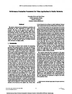
Figure 1: Full Flex board with a dsPIC33 micro-controller.

thresholds, and Earliest Deadline First (EDF) which can be used to schedule periodic tasks with real-time requirements (time-triggered schedule). In addition, it can handle the interrupts that are raised by the I/O interfaces, internal events and timers which allows linking a handler written by the user into an interrupt vector in order to schedule aperiodic tasks (eventdriven scheduling). Erika kernel consist of two layers: the Kernel Layer and the Hardware Abstraction Layer (HAL). The Kernel Layer contains a set of modules that implement task management and real-time scheduling policies. The Hardware Abstraction Layer contains the hardware dependent code that handles context switches and interrupt handling. The Microchip dsPIC33 micro-controller family is supported by the Erika kernel HAL. The Microchip dsPIC33 micro-controller is a high-performance 16-bit digital signal controller (DSC) designed for embedded systems solutions. Specifically an embedded board for dsPIC33 named Full Flex has been used as the hardware experimental platform, see Figure 1. The Full Flex board mounts a Microchip dsPIC33 micro-controller, and exports almost all the pins of the micro-controller. The Full Flex board, integrates an extra-robust power supply circuitry, which allows the usage of a wide range of power suppliers. It accepts voltage ranges between 9-36V. The power supply signal is filtered and adapted to the internal levels. Finally, it is important to stress that the surveyed results in Tables 1 7

and 2 also showed the diversity of controlled plants that have been used. For the selection of the plant, a few factors were considered. First, many standard basic and advanced controller design methods rely on the accuracy of the plant mathematical model. The more accurate the model, the more realistic the simulations, and the better the observation of the effects of the controller on the plant. Hence, the plant was selected among those for which an accurate mathematical model could easily be derived. Plants such as an inverted pendulum or a direct current motor are the defacto plants for benchmark problems in control engineering. However, their modeling is not trivial and the resulting model is often not accurate. Second, it was desired to have a plant that could directly be plugged into a micro-controller without using intermediate electronic components. That is, the transistortransistor logic (TTL) level signals provided by the micro-controller should be enough to carry out the control. Note that this is not the case, for example, for many mechanical systems. Such a simplification in terms of hardware reduces the modeling effort to study the plant and no models for actuators or sensors are required. Third, it was also desired to have a plant that can be easily reproduced, that is, it is easy and cheap to built. Regarding all this requirements, the election was an electronic circuit in the form of a double integrator. Further details will be given in Subsection 3.4.

3

Evaluation framework

This section describes the characteristics of the proposed performance evaluation framework. First, the general services provided by the framework are presented and then the evaluation parameters used in the framework for performance comparison purposes are introduced. Afterward, the design and implementation of the performance evaluation framework is presented.

3.1

Framework services

This section describes the common characteristics that both, the simulation part and the experimental part have to fulfill. To this extend, several services have been identified. Framework services refer to the functional modules that constitute the performance evaluation framework. Each functional module performs specific activities that constitute each service. They have been conceptually defined for providing a flexible and scalable evaluation platform. Framework services are baseline configuration, resource manager, task controller, optimization method and performance measurement (see Figure 2). 8

Performance Measurement Optimization Algorithms

Task Controller

Resource Manager Baseline Configuration

Figure 2: Framework functional modules.

3.1.1

Baseline configuration

The baseline configuration module is responsible for providing an interface between the plants and the other functional models. The proposed framework considers the case of a single processor with multitasking capabilities controlling several continuous plants, as showed in Figure 3 for the case of three plants. This configuration is defined in this module. However, other cases can be supported if a new configuration is defined within this module, e.g. multiple-processors controlling one plant each, or multiple-processors operating as network nodes. The module defines the connectivity between the processor and the plants, this includes analog lines, analog to digital converters, and digital to analog converters. 3.1.2

Resource manager and optimization method

The resource manager module obtains the system dynamics information in the form of kernel workload, plant error (instantaneous or finite horizon), plant measurement state or any system feedback information used to reallocate resources. Using this information, the resource manager executes the previously selected optimization algorithm (see Figure 4). The optimization method module is conformed by a repository of algorithm routines. In particular, the algorithms shown in Table ?? have been implemented. Each algorithm represent a specific FBS or EDC approach. Off-line optimization algorithms are executed just once during the system initialization process, meanwhile on-line optimization algorithms are executed periodically (mainly

9

Baseline Configuration

Processor Task 1

Task 2

Task3

Plant 1

Plant 2

Plant 3

Figure 3: Framework multitasking single processor configuration.

Algorithms

Resource Manager

Selected Algorithm

Baseline Configuration

Figure 4: Framework resource manager module.

for FBS approaches) or aperiodically (for EDC approaches). The optimization module receives the system dynamics information from the resource manager, then the optimization procedure results are sent to the task controller to indicate new settings such as new values for task periods or new controller gains. 3.1.3

Task controller

The task controller module is the responsible to create task instances according to a specific task model (see Figure 5). A set of control task models definitions are available in this module, such as naif, one-sample, split, switching and one-shot task models. Task instances support both periodic and aperiodic interruptions. Timing parameters for the task instances can also be modified on-line by the optimization method module. This module 10

Task Model

Task Controller

Task Task Task instance 1 instances instances

Baseline Configuration

Figure 5: Framework task controller module.

indicates to the baseline configuration module when the different activities within each closed loop operation must be executed, that is, when sampling, control and actuation actions must take place. 3.1.4

Performance measurement

The performance measurement module is able to obtain information from any of the other modules. Raw information such as algorithm execution time, plants’ errors and plants’ states are processed by this module in order to perform a complete assessment using proper metrics to evaluate control performance, resource utilization and computational overhead. This module allows performance evaluation of any resource/performance-aware policy under similar circumstances, providing a fair comparison among them. It can be tuned to process different system (computer and/or plant) data, and to evaluate using alternative metrics. For simulations, control performance is measured using a continuous standard quadratic cost function Z teval  T  x (t)Qx(t) + uT (t)Ru(t) dt. (1) Jcontrol = 0

where the Q and R represents the cost weighting matrices and teval the simulation period. For experiments, control performance is obtained from a discrete-time quadratic cost function d Jcontrol

=

tX eval k=0



 xT (k)Qd x(k) + 2xT (k)Nd u(k) + uT (k)Rd u(k) , 11

(2)

where the Qd ,Nd and Rd represent the discrete cost weighting matrices. Since the experimental platform uses the micro-controller to measure periodically the plant states, then a discrete cost function is required. Meanwhile the simulation platform is capable of obtaining continuous measurements directly from the plant. Resource utilization is measured as a percentage of use of the processor during each evaluation period (teval ). So the resource utilization is defined as ! n 1 X Jresource = (3) Ei ∗ 100, teval i=1

where n is the number of tasks sharing the same processor, and E corresponds to either the total processor time assigned to a specific control task during the simulation period or the total processor time measured for a specific control task during the experimentation period. Therefore, for each specific control task, the total processor time (assigned or measured) is E=

m X

Cj

(4)

j=1

where m is the number of times that a specific control task is invoked during the simulation/execution period, and C corresponds to the task execution time. Computational overhead is included in this parameter. A performance index is defined in order to incorporate control performance and the resource utilization in one metric. Therefore performance index for simulation is defined by P I = Jcontrol ∗ Jresource ,

(5)

and performance index for experiments is defined by d P I d = Jcontrol ∗ Jresource .

3.2

(6)

Framework design and implementation: simulation part

The simulation platform implementing the required services can be described from two main views. The structural view defines the static elements that integrate the platform, meanwhile the execution view defines the sequence of events or steps conducted during the simulation process. The software for the simulation platform can be found at http://dcs.upc.es/uploads/ projects/soft/Platform.zip. 12

Feedback Signal 1

Control Output 1 Control Output 2

Control Signal 1

Sy stem Output 1

Control Signal 2

Sy stem Output 2

Control Signal 3

Sy stem Output 3

Measurement In 1 Total Cost Out

TotalCost

CPU Time Out

CPUTime

Measurement In 2

Feedback Signal 2 Control Output 3 Feedback Signal 3

CPU Load Output

Controlled Plant

Processor Kernel

Measurement In 3 Load Measurement

Measurement System

Figure 6: Simulink/TrueTime model

From a structural view the simulation platform has two levels. Matlab programs running in the Matlab is the first level. Simulink blocks and the TrueTime elements running in the Simulink environment represent the second level. Matlab programs are physically and logically grouped in five main folders. The root folder contains the main program which represents the simulation starting point and it contains configuration files for timing and disturbance data, and plant model definition. The resource manager folder and task controller folder contains programs which are triggered by Simulink/TrueTime blocks. The optimization algorithms and the task models folders represents a repository of programs that implement different EDC and FBS strategies. Partial Matlab source code for main modules can be found at Appendix A. The Simulink/TrueTime model is composed by three elements: processor kernel, controlled plant and measurement system (see Figure 6 for the model in the case of three control tasks). The processor kernel sends control signals to the plants, plants send feedback information to the processor, and the measurement system is capable of obtaining metrics from the other two main blocks. The processor kernel simulates a multitasking processor with a real-time operating system (see Figure 7 for details of this block in the scenario of three control loops). Internally this block is composed by a task controller and a resource manager. The task controller is in charge of the creation of task instances based on a specific control task model. Resource manager obtains feedback information and executes a specific resource optimization algorithm and modifies tasks’s controllers timing parameters if required by the algorithm. The controlled plants group contains a Simulink space-state block for each plant being under control. Each plant can be affected by

13

1 Schedule D/A

A/D

emu

Snd Interrupts

Control Output 1 2

Schedule

Control Output 2 3

Monitors

Control Output 3

Rcv

P

Task Controller

1 Feedback Signal 1 2 Feedback Signal 2 3

A/D Interrupts

D/A

4

Snd

CPU Load Output

Schedule Monitors

Rcv

RM View

emu

P

Feedback Signal 3 Resource Manager

Figure 7: Processor kernel model

disturbance data which is feed during run-time. For the current implementation, it is assumed that plant states are available and therefore there is no need for observers. However if required, observers and estimators can be incorporated in this block. The measurement system block contains two elements, one to measure control performance and the other to measure processor load. Basically each element integrates the individual measurements using the defined cost functions and stores the results in a data structure. If there is a need for additional metrics, this module can be enhanced to support them. From an execution point of view, the simulation platform can be described with the flow diagram showed in Figure 8. Each element in the diagram has the following description: • System configuration. During this step the main configuration parameters are selected, including the control task model (naif, one-shot, one-sample, etc.), the resource optimization algorithm (static, optimal, event-driven) and the plant model. This configuration section contains the definition of the system model, the configuration is modified each time a new model is simulated. • Valid configuration. Once the parameters are selected a validation 14

Start

System Configuration

NO

valid conf ?

YES

Load Data

Execute Simulation

Generate Partial Results

Summarize results and plot

NO

more data?

YES

End

Figure 8: Simulation framework flow diagram

process is executed in order to verify that the selected parameters are correct, e.g. whether the selected task model supports the selected resource optimization algorithm. If the configuration is not valid the system execution ends. • Load data. Before the simulation execution, the timing and disturbance data must be loaded into the system. This data indicates how many execution runs will be conducted, how long each simulation will last, when and how many set-point changes or disturbances will appear during the execution time, or what the magnitude of each disturbance or new set point is. All this information should be previously generated, usually in a random procedure, and stored in a specific file. • Execute simulation. Once configuration and data is ready, the simulation is executed. The simulation consists in the upload and execution of the Simulink/TrueTime model. This model is generic for all simu15

lations. What it makes the difference is the parameters received from the system configuration and load data blocks. • Generate partial results. When a simulation run is completed partial results are stored in a data structure. This partial results include information such as tasks execution time and control performance. • More data. The system verifies if there is more data available for a next simulation. If all data loaded has been already used, then the system proceeds to summarize the results (using the plot block). If there is data available, another simulation run is executed. In this way, different simulation scenarios can be executed for the same system model, and also the same scenarios can be used later on for other models. • Summarize results and plot. Finally, the accumulated data is processed and summarized in order to provide results and plots which represents the performance of the specific system model.

3.3

Framework design and implementation: experimental part

The experimental platform environment can be divided into two main configurations: run-time and programming, as it allows easy and scalable implementation of different resource aware policies. The software for the experimental platform can be found in http://dcs.upc.es/uploads/projects/ soft/Platform.zip. The run-time configuration defines the elements used during the micro-controller execution time. This configuration provides an adequate connectivity among the hardware elements in order to execute the control tasks and extract the evaluation data from the plants through the micro-controller. The programming configuration refers to the microcontroller code generation process, it provides an adequate environment to program, compile and download the software that will run in the dsPIC33 micro-controller for the different policies. 3.3.1

Run-time configuration

In the run-time configuration the Matlab IDE (Integrated Development Environment) is used as an interactive environment that enables the user to perform computationally intensive tasks. Matlab provides key parameters

16

dsPIC33

Task Sample

ADC

Plant Control Actuate

PWM

Figure 9: A micro-controller task controlling one double integrator plant.

and receives on-line information from the micro-controller. A Matlab program (m-file) is executed in order to trigger the execution of the microcontroller program. During the micro-controller execution, Matlab is receiving raw data about control performance and processor load. This data is then processed in order to generate plots and obtain summarized information regarding the behavior of the embedded control system which is conformed by the micro-controller and the controlled plants. In the dsPIC33 micro-controller several task instances area created, each one controlling one plant. The case of one task controlling an electronic double integrator systems is illustrated in Figure 9. Each task is configured in order to be scheduled by the kernel. When a task job is executed, three activities are performed. First, the controlled plant is sampled by reading a value from the micro-controller ADC (Analog-to-Digital Converter) which is connected to the plant output, then it calculates the control signal value according to a specific algorithm, and finally it sends the control action through the microcontroller PWM (Pulse-Width-Modulator) that is connected to the plant input. The hardware for the controlled plants is implemented in the daughter board. According with the performance evaluation framework design, the performance measurement module is constituted by the Matlab IDE, the m-file, and the plots and results. Meanwhile the disPIC33 micro-controller constitutes the implementation of the baseline configuration, resource manager, task controller and optimization algorithms modules.

17

3.3.2

Programming configuration

The programming configuration is composed by the following elements: Erika kernel, source code, Eclipse/RT Druid, MPLAB IDE (Integrated Development Environment) and ICD2 (In-Circuit Debugger), and the Full Flex board. Erika and the Full Flex board equipped with the dsPIC33 Microcontroller were described in Section 2. The source code is the main part of the programming configuration and it is composed by three files embedded in a project: 1)conf.oil that contains the system configuration and the tasks, counters and alarm definition using OIL (OSEK Implementation Language); 2)code.c that represents the source code main program, contains the controller specific activities using C language; 3)setup.c contains a group of common-used functions for the Full Flex board. Main source code functions and definitions can be found at Appendix B. Additional sources files may be added to enhance system functionality. Besides, MPLAB IDE [?], that is an integrated tool-set for the development of embedded applications employing Microchip’s micro-controllers, is used to import the object file produced by the compilation of the source code in the Eclipse/RT-Druid [?] environment, and to download the program to the dsPIC33 micro-controller trough the MPLAB In-Circuit Debbuger (ICD2) interface [?]. 3.3.3

Code details

The main services implemented in the experimental platform inside of the code.c source file are described next. The generation of time in Erika is based on the Timer1 register, which is programmed to rise an interruption every tick (1ms). The interrupt handler is the CounterTick function that shoots the diverse programmed alarms. Each alarm has an associated task, which is then activated for execution. The task can be programmed to be executed just once (aperiodic task) or repeatedly (periodic task). The overall code has been divided into 5 tasks: TaskReferenceChange: periodic task that generates the reference signal by modifying the plant set-point. TaskPeriodicController: periodic task that implements a time-triggered controller. This task is used when implementing any FBS approach. TaskOnlineOptimization: periodic task that executes on-line optimization activities used for some FBS approaches.

18

Algorithm 1: int main(void) begin Clock setup() Timer1 program() Full Flex setup() SetRelAlarm(AlarmReferenceChange, 1000, 1000) SetRelAlarm(AlarmPeriodicController, 1000, 50) SetRelAlarm(AlarmOnlineOptimization, 1000, 10) SetRelAlarm(AlarmEventController, 1000, 0) SetRelAlarm(AlarmSend, 1000, 5) while(1) begin background activities (if any) should go here end end

Figure 10: Main program pseudo-code TaskEventController: aperiodic task that implements a event-driven controller. This task is used when implementing any EDC approach. TaskSend: periodic task that sends plant state information from the dsPIC33 to the PC using RS232 serial communication. The main code initializes software and hardware components (such as clock, timer, ADC), configures alarms and activate tasks, as shown in the pseudo-code of Figure 10. The SetRelAlarm primitive is used to fire an alarm which activates a task with an specific offset and periodicity value, if periodicity is zero the task is executed just once. For example the alarm AlarmEventController activates the task TaskEventController after an offset of 1000ms and it is executed once, meanwhile the alarm AlarmPeriodicController activates the task TaskPeriodicController that is periodically executed every 50ms after an offset of of 1000ms. The TaskPeriodicController implements the controller code for a periodic task (Figure 11). First, it reads the reference signal value (set-point), then it reads the plant state variables through the dsPIC33 ADC. The tracking error is calculated using the state variables and the set-point. Later, it calculates the control signal u using the controller gain L, and finally it sets the PWM duty cycle according with the control signal. The TaskOnlineOptimization executes on-line optimization activities according to the specifications given by a particular FBS approach. If re19

Algorithm 2: TASK(TaskPeriodicController) begin Read reference() Read state() Obtain tracking error() u=Calculate control signal() Apply control signal(u) end

Figure 11: Periodic controller pseudo-code Algorithm 3: TASK(TaskOnlineOptimzation) begin status=Obtain plant or processor status() new period=Optimzation process(status) if ( new period current period ) begin Update controller gain() CancelAlarm(AlarmPeriodicController) SetRelAlarm(AlarmPeriodicController, new period, new period); ActivateTask(TaskPeriodicController); end old period=current period end

Figure 12: On-line optimization pseudo-code quired, this task is capable to modify the task periodicity by canceling the current alarm and releasing the alarm with a new task activation period. The pseudo-code in Figure 12, shows a generic optimization tasks which first obtains the plant state or the processor status in order to conduct the optimization process; then if a new task period is obtained, the controller gain L is updated and a new task period is set. The TaskEventController implements the controller code for an aperiodic task (Figure 13). Notice that according to the code shown in Figure 10, the alarm that activates the task has been configured to be executed once. The code is similar to the TaskPeriodicController, however, at the end, it computes its next activation time via Calculate next activation time function, and it uses this value to set the associated alarm. This code correspond to a self-triggered approach, but it can also support event-triggered approaches by attaching this task to an external interrupt handler. 20

Algorithm 4: TASK(TaskEventController) begin Read reference() Read state() Obtain tracking error() u=Calculate control signal() Apply control signal(u) Event time = Calculate next activation time() SetRelAlarm(AlarmEventController, Event time, 0) end

Figure 13: Event controller pseudo-code

Figure 14: Electronic double integrator circuit

3.4

Plant details

For both simulation and experimental parts, an electronic circuit in the form of a double integrator has been used as a controlled plant. Figure 14 shows the physical implementation of the double integrator. Note that in the integrator configuration, the operational amplifiers require positive and negative input voltages. Otherwise, they will quickly saturate. However, since the circuit is powered by the dsPIC33, and thus no negative voltages are available, the 0V voltage (Vss ) in the non-inverting input has been shifted from GND to half of the value of Vcc (3.3V) by using a voltage divider R3 . Therefore, the operational amplifier differential input voltage can take positives or negatives values. The nominal electronic components values are shown in Table 3. The operational amplifier in integration configuration can be modelled

21

Component R3 R1 R2 C1 C2

Nominal value 1kΩ 100kΩ 100kΩ 470nF 470nF

Table 3: Electronic components nominal values by Vout =

Z

t

− 0

Vin dt + Vinitial RC

(7)

where Vinitial is the output voltage of the integrator at time t = 0, and ideally Vinitial = 0, and Vin and Vout are the input and output voltages of the integrator, respectively. Taking into account (7), and the scheme shown in Figure 14, the double integrator plant dynamics can be modeled by dv2 dt dv1 dt

−1 u R2 C 2 −1 v2 R1 C 1

= =

In continuous-time state-space form,  x˙ = Ax(t) + Bu(t) y(t) = Cx(t) the model is 

v˙ 1 v˙ 2



=



0 0

−1 R1 C1



0    v1 1 0 y = v2

v1 v2 



+

(8)



0 −1 R2 C2



u

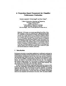
The model validation has been performed by applying a standard control algorithm with a sampling period of h = 50ms, with reference changes, and comparing the theoretical results obtained from a Simulink model with those obtained from the plant. With the validated values for the components, the

22

1 reference v1 v2 u

voltage (V)

0.5

0

-0.5

-1

1.5

2

2.5

3

3.5

4

t(s)

(a) Theoretical simulated plant response 1 reference v1 v2 u

voltage (V)

0.5

0

-0.5

-1

1.5

2

2.5

3

3.5

4

t(s)

(b) Experimental plant response

Figure 15: Model validation. model used for controller design is given by     0 −21.2766 0 x˙ = x+ u 0 0 −21.2766   1 0 x y =

(9)

where the state vector is x = [v1 v2 ]T . Figure 15 shows the results of this validation. In particular, the controller gain L is obtained using linear quadratic (LQ) optimal design which minimizes a discrete cost function equivalent to the continuous cost function in (1) with Q being the identity and R = 1, for the different sampling period choices. Since the voltage input of the operational amplifier is 1.6V (which is half Vcc : the measured Vcc is 3.2V although it is powered by 3.3V), the tracked reference signal has been established to be from 1.1V to 2.1V (±0.5V around 1.6V). 23

uss

Nu r

Nx

+

xr +

K +

−

u

x

plant

C

yr

The goal of the controller is to make the circuit output voltage (v1 in Figure 14) to track a reference signal by giving the appropriate voltage levels (control signals) u. Both states v1 and v2 can be read via the ADC port of the micro-controller and u is applied to the plant through the PWM output. For tracking a reference signal, a tracking structure must be used. Knowing that the discretization of (8) with period h is  xk+1 = Φ(h)xk + Γ(h)uk (10) yk = Cxk where Φ(t) and Γ(t) can be obtained, with t = h, from Φ(t) = eAt Z t eAs Bds, Γ(t) = 0

a common tracking structure [59] is illustrated in Figure 3.4. In this configuration, Nu is the matrix for the feed-forward signal to eliminate steady-state errors, Nx is the matrix that transforms the reference r into a reference state, K is the state feedback gain and C is the plant output matrix. Recall that Nx and Nu can be computed in the continuous-time domain as 

Nx Nu



=



A B C 0

−1 

0 1



while in the discrete-time domain are computed as 

Nx Nu



=



Φ−I Γ C 0

−1 

0 1



For the  double  integrator tracking, the feed-forward matrix Nu is zero and Nx = 1 0 . 24

4

Conclusions

This report has described a framework aimed at evaluating whether state of the art results on resource and performance aware policies for embedded control systems can be implemented in practice.

References [1] Seto D, Lehoczky J, Sha L, Shin K (1996) On task schedulability in real-time control systems. In: Real-Time Systems Symposium, 1996., 17th IEEE, pp 13 –21 [2] Seto D, Lehoczky JP, Sha L (1998b) Task period selection and schedulability in real-time systems. In: Proceedings of the IEEE Real-Time Systems Symposium, RTSS ’98 [3] Zhao QC, Zheng DZ (1999) Stable and real-time scheduling of a class of hybrid dynamic systems. Discrete Event Dynamic Systems 9:45–64 [4] Eker J, Hagander P, ˚ Arz´en KE (2000) A feedback scheduler for realtime controller tasks. Control Engineering Practice 8(12):1369 – 1378 [5] Rehbinder H, Sanfridson M (2000) Integration of off-line scheduling and optimal control. In: Proceedings of the 12th Euromicro conference on Real-time systems, pp 137–143 [6] Henriksson D, Cervin A, ˚ Akesson J, ˚ Arz´en KE (2002) Feedback scheduling of model predictive controllers. In: Proceedings of the Eighth IEEE Real-Time and Embedded Technology and Applications Symposium (RTAS’02) [7] Palopoli L, Pinello C, Sangiovanni Vincentelli A, Elghaoui L, Bicchi A (2002b) Synthesis of robust control systems under resource constraints. In: Tomlin C, Greenstreet M (eds) Hybrid Systems: Computation and Control, Lecture Notes in Computer Science, vol 2289, Springer Berlin / Heidelberg, pp 197–225 [8] Cervin A, Eker J, Bernhardsson B, ˚ Arz´en KE (2002) Feedbackfeedforward scheduling of control tasks. Real-Time Syst 23:25–53 [9] Chandra R, Liu X, Sha L (2003) On the scheduling of flexible and reliable real-time control systems. Real-Time Syst 24:153–169 25

[10] Mart´ı P, Lin C, Brandt SA, Velasco M, Fuertes JM (2004) Optimal state feedback based resource allocation for resource-constrained control tasks. In: Proceedings of the 25th IEEE International Real-Time Systems Symposium, pp 161–172 [11] Palopoli L, Pinello C, Bicchi A, Sangiovanni-Vincentelli A (2005) Maximizing the stability radius of a set of systems under real-time scheduling constraints. Automatic Control, IEEE Transactions on 50(11):1790 – 1795 [12] Henriksson D, Cervin A (2005) Optimal on-line sampling period assignment for real-time control tasks based on plant state information. In: Decision and Control, 2005 and 2005 European Control Conference. CDC-ECC ’05. 44th IEEE Conference on, pp 4469 – 4474 [13] Casta˜ n´e R, Mart´ı P, Velasco M, Cervin A (2006) Resource management for control tasks based on the transient dynamics of closed-loop systems. In: Proceedings of the 18th Euromicro Conference on RealTime Systems, pp 171–182 [14] Ben Gaid M, Cela A, Hamam Y, Ionete C (2006) Optimal scheduling of control tasks with state feedback resource allocation. In: American Control Conference, 2006 [15] Bini E, Cervin A (2008) Delay-aware period assignment in control systems. In: Proceedings of the 2008 Real-Time Systems Symposium, pp 291–300 [16] Samii S, Cervin A, Eles P, Peng Z (2009a) Integrated scheduling and synthesis of control applications on distributed embedded systems. In: Proceedings of the Conference on Design, Automation and Test in Europe, pp 57–62 [17] Samii S, Eles P, Peng Z, Cervin A (2009b) Quality-driven synthesis of embedded multi-mode control systems. In: Proceedings of the 46th Annual Design Automation Conference, pp 864–869 [18] Mart´ı P, Lin C, Brandt SA, Velasco M, Fuertes JM (2009a) Draco: Efficient resource management for resource-constrained control tasks. IEEE Transactions on Computers 58:90–105 [19] Ben Gaid MM, Cela A, Hamam Y (2009) Optimal real-time scheduling of control tasks with state feedback resource allocation. Control Systems Technology, IEEE Transactions on 17(2):309 –326 26

[20] Cervin A, Velasco M, Marti P, Camacho A (2011) Optimal online sampling period assignment: Theory and experiments. Control Systems Technology, IEEE Transactions on 19(4):902 – 910 ˚rz´en KE (1999) A simple event-based PID controller. In: Preprints [21] A 14th World Congress of IFAC, Beijing, P.R. China [22] Heemels WPMH, Gorter RJA, van Zijl A, van den Bosch PPJ, Weiland S, Hendrix WHA, Vonder MR (1999) Asynchronous measurement and control: a case study on motor synchronization. Control Engineering Practice 7(12):1467 – 1482 [23] ˚ Astr¨ om K, Bernhardsson B (2002) Comparison of riemann and lebesgue sampling for first order stochastic systems. In: Decision and Control, 2002, Proceedings of the 41st IEEE Conference on, vol 2, pp 2011 – 2016 vol.2 [24] Velasco M, , Mart´ı P, Fuertes J (2003) The self triggered task model for real-time control systems. In: Work-in-progress session of the 24th IEEE Real-Time Systems Symposium [25] Tabuada P, Wang X (2006) Preliminary results on state-trigered scheduling of stabilizing control tasks. In: Decision and Control, 2006 45th IEEE Conference on, pp 282 –287 [26] Miskowicz M (2006) Send-on-delta concept: an event-based data reporting strategy. Sensors 6:49–63 [27] Tabuada P (2007) Event-triggered real-time scheduling of stabilizing control tasks. Automatic Control, IEEE Transactions on 52(9):1680 – 1685 [28] Lemmon M, Chantem T, Hu X, Zyskowski M (2007) On self-triggered full-information h-infinity controllers. In: Bemporad A, Bicchi A, Buttazzo G (eds) Hybrid Systems: Computation and Control, Lecture Notes in Computer Science, vol 4416, Springer Berlin / Heidelberg, pp 371–384 [29] Johannesson E, Henningsson T, Cervin A (2007) Sporadic control of first-order linear stochastic systems. In: Proc. 10th International Conference on Hybrid Systems: Computation and Control, Springer-Verlag, Pisa, Italy

27

[30] Suh YS, Nguyen VH, Ro YS (2007) Modified kalman filter for networked monitoring systems employing a send-on-delta method. Automatica 43(2):332 – 338 [31] Anta A, Tabuada P (2008a) Self-triggered stabilization of homogeneous control systems. In: Proceedings of the American Control Conference [32] Anta A, Tabuada P (2008b) Space-time scaling laws for self-triggered control. In: Decision and Control, 2008. CDC 2008. 47th IEEE Conference on, pp 4420 –4425 [33] Wang X, Lemmon M (2008a) Event design in event-triggered feedback control systems. In: Decision and Control, 2008. CDC 2008. 47th IEEE Conference on, pp 2105 –2110 [34] Wang X, Lemmon MD (2008b) State based self-triggered feedback control systems with l2 stability. In: 17th IFAC World Congress [35] Heemels WPMH, Sandee JH, Bosch P (2008) Analysis of event-driven controllers for linear systems. International Journal of Control 84(1) [36] Henningsson T, Johannesson E, Cervin A (2008) Sporadic eventbased control of first-order linear stochastic systems. Automatica 44(11):2890–2895 [37] Wang X, Lemmon M (2009a) Self-triggered feedback control systems with finite-gain l2 stability. Automatic Control, IEEE Transactions on 54(3):452 –467 [38] Wang X, Lemmon M (2009b) Self-triggered feedback systems with state-independent disturbances. In: American Control Conference, 2009. ACC ’09., pp 3842 –3847 [39] Mart´ı P, Velasco M, Bini E (2009b) The optimal boundary and regulator design problem for event-driven controllers. In: Majumdar R, Tabuada P (eds) Hybrid Systems: Computation and Control, Lecture Notes in Computer Science, vol 5469, Springer Berlin / Heidelberg, pp 441–444 [40] Mazo M, Ant A, Tabuada P (2009) On self-triggered control for linear systems: Guarantees and complexity. In: 10th European Control Conference

28

[41] Mazo M, Tabuada P (2009) Input-to-state stability of self-triggered control systems. In: Decision and Control, 2009 held jointly with the 2009 28th Chinese Control Conference. CDC/CCC 2009. Proceedings of the 48th IEEE Conference on, pp 928 –933 [42] Velasco M, Mart´ı P, Bini E (2009b) On lyapunov sampling for eventdriven controllers. In: Decision and Control, 2009 held jointly with the 2009 28th Chinese Control Conference. CDC/CCC 2009. Proceedings of the 48th IEEE Conference on, pp 6238 –6243 [43] Anta A, Tabuada P (2009) Isochronous manifolds in self-triggered control. In: Decision and Control, 2009 held jointly with the 2009 28th Chinese Control Conference. CDC/CCC 2009. Proceedings of the 48th IEEE Conference on, pp 3194 –3199 [44] Anta A, Tabuada P (2010) To sample or not to sample: Self-triggered control for nonlinear systems. Automatic Control, IEEE Transactions on 55(9):2030 –2042 [45] Lozoya C, Velasco M, Mart´ı P (2008b) The one-shot task model for robust real-time embedded control systems. Industrial Informatics, IEEE Transactions on 4(3):164 –174 [46] Lozoya C, Velasco M, Mart´ı P (2007) A 10-year taxonomy on prior work on sampling period selection for resource-constrained real-time control systems. In: Work in Progress 19th Euromicro Conference on Real-Time Systems [47] Marau R, Leite P, Velasco M, Mart´ı P, Almeida L, Pedreiras P, Fuertes J (2008) Performing flexible control on low-cost microcontrollers using a minimal real-time kernel. Industrial Informatics, IEEE Transactions on 4(2):125 –133 [48] Cervin A, Alriksson P (2006) Optimal on-line scheduling of multiple control tasks: A case study. In: Proceedings of the 18th Euromicro Conference on Real-Time Systems, Dresden, Germany [49] Velasco M, Mart´ı P, Lozoya C (2008b) On the timing of discrete events in event-driven control systems. In: Proceedings of the 11th international workshop on Hybrid Systems: Computation and Control, HSCC ’08, pp 670–673

29

[50] Velasco M, Mart´ı P, Bini E (2009a) Equilibrium sampling interval sequences for event-driven controllers. In: European Control Conference 2009 [51] Velasco M, Mart´ı P, Fuertes JM, Lozoya C, Brandt SA (2010) Experimental evaluation of slack management in real-time control systems: Coordinated vs. self-triggered approach. J Syst Archit 56:63–74 [52] Department of Automatic Control Lund University. Truetime: Simulation of networked and embedded control systems. http://www. control.lth.se/truetime/, 2010. [53] MathWorks. Matlab and Simulink for technical computing. http: //www.mathworks.com, 2010. [54] Evidence Srl. ERIKA Enterprise basic manual. http://www.evidence. eu.com, 2008. [55] Evidence Srl. FLEX Modular solution for embedded applications. http://www.evidence.eu.com, 2008. [56] Microchip. dsPIC30F/33F Programmer’s Reference Manual. http: //www.microchip.com, 2005. [57] Mart´ı P, Velasco M, Fuertes J, Camacho A, Buttazzo G (2010) Design of an embedded control system laboratory experiment. Industrial Electronics, IEEE Transactions on 57(10):3297 –3307 [58] OSEK. Osek/vdx: Open systems and the corresponding interfaces for automotive electronics. http://www.osek-vdx.org/mirror/os21. pdf. [59] ˚ Astr¨ om KJ, Wittenmark B (1997) Computer-controlled systems: theory and design. Prentice-Hall, Inc.

30

A

Appendix: Framework simulation source code

This appendix presents partial source code for the main files that conforms the simulation part of the performance evaluation framework.

A.1 A.1.1

Main program Function: main.m

Function : main Description : Evaluate

d i f f e r e n t FBS and DCS methods

%−−−−−−−−−−−−−−−−−−−−−−−−−−−−−−−−−−−−−−−−−−−−−−−−−−−−− % V a l i d a t e models %−−−−−−−−−−−−−−−−−−−−−−−−−−−−−−−−−−−−−−−−−−−−−−−−−−−−− validate models ; %−−−−−−−−−−−−−−−−−−−−−−−−−−−−−−−−−−−−−−−−−−−−−−−−−−−−− % Load d i s t r u b a n c e d a t a %−−−−−−−−−−−−−−−−−−−−−−−−−−−−−−−−−−−−−−−−−−−−−−−−−−−−− l o a d d i s t u r b a n c e d a t a ; a m p l i t u d e v a l u e s = load ( a m p l i t u d e f i l e ) ; d e l a y v a l u e s = load ( d e l a y f i l e ) ; %−−−−−−−−−−−−−−−−−−−−−−−−−−−−−−−−−−−−−−−−−−−−−−−−−−−−− % C r e a t e p l a n t and % e x e c u t e o f f −l i n e o p t i m i z a t i o n i f a p p l i e s %−−−−−−−−−−−−−−−−−−−−−−−−−−−−−−−−−−−−−−−−−−−−−−−−−−−−− switch plant used case { ’ r c c i r c u i t ’} plant RC ; case { ’ ball beam ’ } plant BB ; case { ’ double integrator ’} plant DI ; otherwise disp ( ’ S e l e c t a v a l i d p r o c e s s p l a n t ! ! ! ! ’ ) ; pause ; end %−−−−−−−−−−−−−−−−−−−−−−−−−−−−−−−−−−−−−−−−−−−−−−−−−−−−− % Display i n i t i a l values 31

%−−−−−−−−−−−−−−−−−−−−−−−−−−−−−−−−−−−−−−−−−−−−−−−−−−−−− i f debug mode == 1 disp ( s p r i n t f ( ’TASK MODEL SELECTED: %s ’ , t a s k m o d e l ) ) ; disp ( s p r i n t f ( ’SCHEDULING APPROACH: %s ’ , f b s a p p r o a c h ) ) ; disp ( s p r i n t f ( ’ INITIAL PERIODS : [ % 8 . 6 f %8.6 f %8.6 f ] ’ , h ( 1 ) , h ( 2 ) , h ( 3 ) ) ) pause ; end f or i e x e c = 1 : 1 : length ( a m p l i t u d e v a l u e s ) %−−−−−−−−−−−−−−−−−−−−−−−−−−−−−−−−−−−−−−−−−−−−−−−−−−−−− % S e l e c t d i s t u r b a n c e a m p l i t u d and d e l a y %−−−−−−−−−−−−−−−−−−−−−−−−−−−−−−−−−−−−−−−−−−−−−−−−−−−−− d i s t u r b a n c e a m p l i t u d e=a m p l i t u d e v a l u e s ( i e x e c , : ) ; d i s t u r b a n c e d e l a y=d e l a y v a l u e s ( i e x e c , : ) ; c p u e n t r i e s =0; switch plant used case { ’ r c c i r c u i t ’} d i s t u r b a n c e t r a c k =0; case { ’ ball beam ’ } d i s t u r b a n c e t r a c k =1; case { ’ double integrtaor ’} d i s t u r b a n c e t r a c k =1; otherwise disp ( ’ S e l e c t a v a l i d p r o c e s s p l a n t ! ! ! ! ’ ) ; pause ; end i f d i s t u r b a n c e t y p e == 1 task offset = disturbance delay ; end %−−−−−−−−−−−−−−−−−−−−−−−−−−−−−−−−−−−−−−−−−−−−−−−−−−−−− % Execute Simulation %−−−−−−−−−−−−−−−−−−−−−−−−−−−−−−−−−−−−−−−−−−−−−−−−−−−−− sim ( ’ f b s s y s t e m ’ , [ i n i t t i m e e n d t i m e ] ) ; s i m r e s u l t s =[ s i m r e s u l t s , T o t a l C o s t ( length ( T o t a l C o s t ) ) ] ; c p u r e s u l t s =[ c p u r e s u l t s , CPUTime( length (CPUTime ) ) ] ; c p u t o t a l e n t r i e s =[ c p u t o t a l e n t r i e s , c p u e n t r i e s ] ; i f debug mode == 1 disp ( s p r i n t f ( ’ Cost Function ’ ) ) ; 32

disp ( s p r i n t f ( ’ %8.6 f ’ ,mean( s i m r e s u l t s ) ) ) ; disp ( s p r i n t f ( ’CPU Load ’ ) ) ; disp ( s p r i n t f ( ’ %8.6 f ’ ,mean( c p u r e s u l t s ) ) ) ; pause ; end end %−−−−−−−−−−−−−−−−−−−−−−−−−−−−−−−−−−−−−−−−−−−−−−−−−−−−− % Display f i n a l r e s u l t s %−−−−−−−−−−−−−−−−−−−−−−−−−−−−−−−−−−−−−−−−−−−−−−−−−−−−− disp ( s p r i n t f ( ’−−−−−−−−−−−−−−−−−−−−−−−−−−−−−−− ’ ) ) ; disp ( s p r i n t f ( ’ Cost Function ’ ) ) ; disp ( s p r i n t f ( ’ Mean Value ’ ) ) ; disp ( s p r i n t f ( ’ %8.6 f ’ ,mean( s i m r e s u l t s ) ) ) ; disp ( s p r i n t f ( ’CPU Load ’ ) ) ; disp ( s p r i n t f ( ’ Mean Value ’ ) ) ; disp ( s p r i n t f ( ’ %6.2 f ’ ,mean( c p u r e s u l t s ) ) ) ;

A.2 A.2.1

Initialization modules Function: task controller init.m

Function : Description :

task controller init I n i t i a l i z e s the Simulink

task

controller

module

function t a s k c o n t r o l l e r i n i t % I n i t i a l i z e TrueTime k e r n e l ttInitKernel (6 , 3 , tc sched dfn ) ; % C r e a t e Tasks switch task model case { ’ fbs ’} ttCreatePeriodicTask ( ttCreatePeriodicTask ( ttCreatePeriodicTask ( case { ’ event ’ } ttCreatePeriodicTask ( ttCreatePeriodicTask ( ttCreatePeriodicTask ( otherwise 33

’ t a s k 1 ’ , 0 . 0 , h ( 1 ) , 1 , ’ f b s c o n t r o l l e r c o d e ’ , da ’ t a s k 2 ’ , 0 . 0 , h ( 2 ) , 1 , ’ f b s c o n t r o l l e r c o d e ’ , da ’ t a s k 3 ’ , 0 . 0 , h ( 3 ) , 1 , ’ f b s c o n t r o l l e r c o d e ’ , da

’ task1 ’ ,0.0 , h (1) ,1 , ’ e v e n t c o n t r o l l e r c o d e ’ , ’ task2 ’ ,0.0 , h (2) ,1 , ’ e v e n t c o n t r o l l e r c o d e ’ , ’ task3 ’ ,0.0 , h (3) ,1 , ’ e v e n t c o n t r o l l e r c o d e ’ ,

disp ( ’ S e l e c t a v a l i d t a s k model ! ! ! ! ’ ) ; pause ; end A.2.2

Function: resource manager init.m

Function : Description :

task controller init I n i t i a l i z e s the Simulink

r e s o u r c e management module

function r e s o u r c e m a n a g e r i n i t

% C r e a t e Tasks switch optimization approach case { ’ s t a t i c ’ , ’ seto edf ’} ttCreatePeriodicTask ( ’ task0 int ’ ,0.0 , null Tfbs ,1 , ’ p e r i od al l oc at case { ’ marti optimal ’} ttCreatePeriodicTask ( ’ t a s k 0 i n t ’ , 0 . 0 , marti Tfbs , 1 , ’ p e r i o d a l l o c a case { ’ h e n r i k s o n f i n i t e ’} ttCreatePeriodicTask ( ’ t a s k 0 i n t ’ , 0 . 0 , henr Tfbs , 1 , ’ p e r i o d a l l o c a t c a s e { ’ e d c v e l a s c o ’ , ’ edc lemmon ’ , ’ e d c m a r t i ’ } ttCreatePeriodicTask ( ’ task0 int ’ ,0.0 , null Tfbs ,1 , ’ p e r i od al l oc a otherwise disp ( ’ S e l e c t a v a l i d s c h e d u l i n g approach ! ! ! ! ’ ) ; pause ; end

A.3 A.3.1

Controllers and optimization algorithms Function: fbs controller code.m

Function : Description :

fbs controller code C o n t r o l t a s k f o r FBS a p p r o a c h e s

function [ e x e c t i m e , data ] = n a i f c o n t r o l l e r c o d e ( seg , data ) s w i t c h seg , case 1 , y1 = t t A n a l o g I n ( data . y1Chan ) ; % Read p r o c e s s o u t p u t y2 = t t A n a l o g I n ( data . y2Chan ) ; % Read p r o c e s s o u t p u t data . u=−Kd( data . task number , : ) ∗ [ y1 ; y2 ; data . y3 ] ; 34

data . y3=data . u ; e x e c t i m e = data . e x e c t i m e ; case 2 , ttAnalogOut ( data . uChan , data . u ) ; % Output c o n t r o l s i g n a l t t S e t P e r i o d ( h ( data . task number ) , data . task name ) ; c p u e n t r i e s=c p u e n t r i e s +1; e x e c t i m e = −1; end A.3.2

File: event controller code.m

Function : Description :

event controller code C o n t r o l t a s k f o r EDC a p p r o a c h e s

function [ e x e c t i m e , data ] = e v e n t c o n t r o l l e r c o d e ( seg , data ) s w i t c h seg , case 1 , y1 = t t A n a l o g I n ( data . y1Chan ) ; % Read p r o c e s s o u t p u t y2 = t t A n a l o g I n ( data . y2Chan ) ; % Read p r o c e s s o u t p u t data . u=−Kd( data . task number , : ) ∗ [ y1 ; y2 ] ; h ( data . task number )= n e x t e v e n t (−Kd( data . task number , : ) , e v e n t p a r e x e c t i m e = data . e x e c t i m e ; case 2 , ttAnalogOut ( data . uChan , data . u ) ; % Output c o n t r o l s i g n a l t t S e t P e r i o d ( h ( data . task number ) , data . task name ) ; c p u e n t r i e s=c p u e n t r i e s +1; e x e c t i m e = −1; end A.3.3

Function: period allocate.m

Function : Description :

period allocate Executed to c a l l

on− l i n e

optimization

routines

function [ e x e c t i m e , data ] = p e r i o d a l l o c a t e ( seg , data ) s w i t c h seg , case 1 , switch fbs approach 35

case { ’ s t a t i c ’ , ’ seto edf ’} data=n u l l a l l o c a t e ( data ) ; c a s e { ’ e d c v e l a s c o ’ , ’ edc lemmon ’ , ’ e d c m a r t i ’ } data=e v e n t a l l o c a t e ( data ) ; case { ’ marti optimal ’} data=o p t i m a l a l l o c a t e ( data ) ; case { ’ h e n r i k s o n f i n i t e ’} data=f i n i t e h o r i z o n a l l o c a t e ( data ) ; otherwise disp ( ’ S e l e c t a v a l i d s c h e d u l i n g approach ! ! ! ! ’ ) ; pause ; end e x e c t i m e = data . e x e c t i m e ; case 2 , e x e c t i m e = −1; end

36

B

Appendix: Framework experiment source code

This appendix presents partial source code for the main files that conforms the experimental part of the performance evaluation framework. The code include functions provided by the Erika kernel.

B.1

File: setup.c

B.1.1

Function: EE Flex setup()

Function : Description :

EE Flex setup () C o n f i g u r e s system

c l o c k and

initialize

devices

void EE Flex setup ( void ) { // C o n f i g u r e t h e PWM 1 PWM init ( ) ; // C o n f i g u r e t h e o r a n g e l e d o f t h e FLEX FULL and custom l e d s Led init (); // C o n f i g u r e d i g i t a l p i n s t o be used with t h e o s c i l l o s c o p e Digital output init (); // I n i t i a l i z e t h e UART Port 1 t o communicate with t h e PC v i a RS232 UART1 DMA init ( ) ; // I n i t i a l i z e t h e Analog t o D i g i t a l C o n v e r t e r 1 ADC1 init ( ) ; } B.1.2

Function: PWM init()

Function : PWM config ( ) D e s c r i p t i o n : C o n f i g u r e s PWM a c t u a t o r

v o i d PWM init ( v o i d ) { OVDCON = 0 x0000 ; // PWM o u t p u t s d i s a b l e d PTCONbits .PTEN = 1 ; //PTEN: PWM Time Base Timer Enable b i t //1 = PWM time b a s e i s on //0 = PWM time b a s e i s o f f PTCONbits .PTMOD=2; //PTMOD: PWM Time Base Mode S e l e c t b i t s 37

//11 =PWM time b a s e o p e r a t e s i n a Continuous Up/ // Count mode with i n t e r r u p t s f o r d o u b l e PWM u p d a //10 =PWM time b a s e o p e r a t e s i n a Continuous Up/ //01 =PWM time b a s e o p e r a t e s i n S i n g l e P u l s e mod //00 =PWM time b a s e o p e r a t e s i n a Free−Running m PTPER = 0x3FFF ; //PTPER: PWM Time Base P e r i o d Value b i t s // S e l e c t PWM p e r i o d : S e t t i n g PDCx=0 means 0% Dut // PDCx=PTPER means 50% // PDCx=2∗PTPER means PWMCON1bits .PMOD1=1;//PWM I /O P a i r Mode b i t s //1 = PWM I /O p i n p a i r i s i n t h e Independent PWM //0 = PWM I /O p i n p a i r i s i n t h e Complementary O PWMCON1bits .PMOD2=1; PWMCON1bits .PMOD3=1; PWMCON1bits .PMOD4=1; PWMCON1bits . PEN4H=1;//PWMxH I /O Enable b i t s //1 = PWMxH p i n i s e n a b l e d f o r PWM output //0 = PWMxH p i n d i s a b l e d , I /O p i n becomes g e n e r a PWMCON1bits . PEN3H=1; PWMCON1bits . PEN2H=1; PWMCON1bits . PEN1H=1; PWMCON1bits . PEN4L=1;//PWMxL I /O Enable b i t s //1 = PWMxL p i n i s e n a b l e d f o r PWM output //0 = PWMxL p i n d i s a b l e d , I /O p i n becomes g e n e r a PWMCON1bits . PEN3L=1; PWMCON1bits . PEN2L=1; PWMCON1bits . PEN1L=1; PWMCON2bits . IUE = 0 ; / / Immediate Update Enable b i t //1 = Updates t o t h e a c t i v e PDC r e g i s t e r s a r e im //0 = Updates t o t h e a c t i v e PDC r e g i s t e r s a r e s y // t o t h e PWM time b a s e PWMCON2bits . UDIS= 0 ; / /PWM Update D i s a b l e b i t //1 = Updates from Duty Cycle and P e r i o d B u f f e r // r e g i s t e r s a r e d i s a b l e d //0 = Updates from Duty Cycle and P e r i o d B u f f e r // r e g i s t e r s a r e e n a b l e d OVDCON = 0 x f f 0 0 ; //OVERRIDE CONTROL REGISTER // b i t 15−8 POVDxH:POVDxL: PWM Output // O v e r r i d e b i t s //1 = Output on PWMx I /O p i n i s c o n t r o l l e d by t h 38

PDC1 = 0 x0000 ; PDC2 = 0 x0000 ; PDC3 = 0 x0000 ; PDC4 = 0 x0000 ; PTCONbits .PTEN

//PWM g e n e r a t o r //0 = Output on PWMx I /O p i n i s c o n t r o l l e d by t h // v a l u e i n t h e c o r r e s p o n d i n g POUTxH:POUTxL b i t // b i t 7−0 POUTxH:POUTxL: PWM Manual Ou //1 = PWMx I /O p i n i s d r i v e n a c t i v e when t h e // c o r r e s p o n d i n g POVDxH:POVDxL b i t i s c l e a r e d //0 = PWMx I /O p i n i s d r i v e n i n a c t i v e when t h e // c o r r e s p o n d i n g POVDxH:POVDxL b i t i s c l e a r e d ∗/ // I n i t i a l duty c y c l e PWM1 // I n i t i a l duty c y c l e PWM2 // I n i t i a l duty c y c l e PWM3 // I n i t i a l duty c y c l e PWM4 = 1 ; // Enable PWM.

} B.1.3

Function: Led init()

Function : Description :

Led init () Configures

FLEX FULL o r a n g e

void L e d i n i t ( void ) { LATBbits . LATB14 = 0 ; TRISBbits . TRISB14 = 0 ;

led

( Jumper 4 must be c l o s e d )

// s e t o r a n g e LED (LEDSYS/RB14) d r i v e s t a t e l // s e t LED p i n (LEDSYS/RB14) a s output

LATDbits . LATD8=0; TRISDbits . TRISD8=0;

// s e t p i n ( IC1 /RD8)−>(CON5/ Pin7 ) d r i v e s t a t e // s e t p i n ( IC1 /RD8)−>(CON5/ Pin7 ) a s output

LATDbits . LATD9=0; TRISDbits . TRISD9=0;

// s e t p i n ( IC2 /RD9)−>(CON5/ Pin10 ) d r i v e s t a t e // s e t p i n ( IC2 /RD9)−>(CON5/ Pin10 ) a s output

LATDbits . LATD10=0; TRISDbits . TRISD10=0;

// s e t p i n ( IC3 /RD10)−>(CON5/ Pin9 ) d r i v e s t a t e // s e t p i n ( IC3 /RD10)−>(CON5/ Pin9 ) a s output

LATDbits . LATD11=0; TRISDbits . TRISD11=0;

// s e t p i n ( IC4 /RD11)−>(CON5/ Pin12 ) d r i v e s t a t // s e t p i n ( IC4 /RD11)−>(CON5/ Pin12 ) a s output

LATDbits . LATD12=0; TRISDbits . TRISD12=0;

// s e t p i n ( IC5 /RD12)−>(CON5/ Pin15 ) d r i v e s t a t // s e t p i n ( IC5 /RD12)−>(CON5/ Pin15 ) a s output

LATDbits . LATD13=0;

// s e t p i n ( IC6 /CN19/RD13)−>(CON5/ Pin18 ) d r i v e 39

TRISDbits . TRISD13=0;

// s e t p i n ( IC6 /CN19/RD13)−>(CON5/ Pin18 ) a s out

} B.1.4

Function: Digital output init()

Function : Digital output init () D e s c r i p t i o n : C o n f i g u r e s p i n (AN10/RB10)−−>(CON6/ Pin 28 ) from t h e FLEX FULL t o g e t e x e c u t i o n t i m e s w i t h o s c i l l o s c o p e

void D i g i t a l o u t p u t i n i t ( void ) { // s e t p i n (AN10/RB10)−−>(CON6/ Pin28 ) d r i v e s t a t e low LATBbits . LATB10 = 0 ; // s e t p i n (AN10/RB10)−−>(CON6/ Pin28 ) a s output TRISBbits . TRISB10 = 0 ; } B.1.5

Function: UART1 DMA init()

Function : UART1 DMA init ( ) D e s c r i p t i o n : I n i t i a l i z e t h e UART P o r t 1 t o communicate w i t h t h e PC v i a RS232

v o i d UART1 DMA init ( ) { cfgDma4UartTx ( ) ; / / This r o u t i n e C o n f i g u r e s DMAchannel 4 f o r t r a n s m i s cfgDma5UartRx ( ) ; / / This r o u t i n e C o n f i g u r e s DMAchannel 5 f o r r e c e p t i o

U1MODEbits . STSEL = 0 ; / / 1−s t o p b i t U1MODEbits . PDSEL = 0 ; / / No P a r i t y , 8−data b i t s U1MODEbits .ABAUD = 0 ; / / Autobaud D i s a b l e d U1MODEbits .BRGH=1;// 1 = BRG g e n e r a t e s 4 c l o c k s p e r b i t p e r i o d ( 4 x b // High−Speed mode ) // 0 = BRG g e n e r a t e s 16 c l o c k s p e r b i t p e r i o d ( 1 6 x // Standard mode ) U1BRG = BRGVAL; // See #i f d e f BITRATE1 above f o r d e t a i l s // C o n f i g u r e UART f o r DMA t r a n s f e r s U1STAbits . UTXISEL0 = 1 ; / / UTXISEL: T r a n s m i s s i o n I n t e r r u p t Mode // 11 =Reserved ; do not u s e // 10 =I n t e r r u p t when a c h a r a c t e r i s t r a n s f e r // Transmit S h i f t R e g i s t e r , and a s a r e s u l t , 40

// b u f f e r becomes empty // 01 =I n t e r r u p t when t h e l a s t c h a r a c t e r i s s // o f t h e Transmit S h i f t R e g i s t e r ; a l l t r a n s m operations

// a r e completed // 00 =I n t e r r u p t when a c h a r a c t e r i s t r a n s f e r // Transmit S h i f t R e g i s t e r ( t h i s i m p l i e s t h e r // one c h a r a c t e r open i n t h e t r a n s m i t b u f f e r ) U1STAbits . URXISEL = 1 ; / / 11 =I n t e r r u p t i s s e t on UxRSR t r a n s f e r mak // r e c e i v e b u f f e r f u l l ( i . e . , has 4 data c h a r // 10 =I n t e r r u p t i s s e t on UxRSR t r a n s f e r mak // r e c e i v e b u f f e r 3/4 f u l l ( i . e . , has 3 data // 0x =I n t e r r u p t i s s e t when any c h a r a c t e r i s // and t r a n s f e r r e d from t h e UxRSR t o t h e r e c e // R e c e i v e b u f f e r has one o r more c h a r a c t e r s . // Enable UART Rx and Tx U1MODEbits .UARTEN = 1 ; / / Enable UART U1STAbits .UTXEN = 1 ; / / Enable UART Tx I E C 4 b i t s . U1EIE = 0 ; // UART1 E r r o r I n t e r r u p t Enable b i t // 1 = I n t e r r u p t r e q u e s t has o c c u r r e d // 0 = I n t e r r u p t r e q u e s t has not o c c u r r e d ∗/ } B.1.6

Function: ADC1 init()

Function : Description :

ADC1 init ( ) C o n f i g u r e s ADC1

v o i d ADC1 init ( v o i d ) {

AD1CON1bits .ADON = 0 ; / / ADC O p e r a t i n g Mode b i t . Turn o f f t h e A/D c o AD1PCFGL = 0xFFFF ; //ADC1 Port C o n f i g u r a t i o n R e g i s t e r Low AD1PCFGH = 0xFFFF ; //ADC1 Port C o n f i g u r a t i o n R e g i s t e r High AD1PCFGLbits . PCFG11=0; // P l an t B ( Double i n t e g r a t o r B) , x1 AD1PCFGLbits . PCFG12=0; // P l an t B ( Double i n t e g r a t o r B) , x2 AD1PCFGLbits . PCFG13=0; // P l an t A ( Double i n t e g r a t o r A) , x1 AD1PCFGLbits . PCFG15=0; // P l an t A ( Double i n t e g r a t o r A) , x2 AD1PCFGHbits . PCFG17=0; // P l an t D (RC−RC D) , x2 AD1PCFGHbits . PCFG18=0; // P l an t D (RC−RC D) , x1 AD1PCFGHbits . PCFG20=0; // P l an t C ( Double i n t e g r a t o r C) , x1 41

AD1PCFGHbits . PCFG21=0; // P l an t C ( Double i n t e g r a t o r C) , x2 AD1CON2bits .VCFG = 0 ;

// C o n v e r t e r V o l t a g e R e f e r e n c e C o n f i g u r a t i o n // ( ADRef+=AVdd, ADRef−=AVss ) AD1CON3bits .ADCS = 6 3 ; // ADC C o n v e r s i o n Clock S e l e c t b i t s / / ( Tad = Tcy ∗ (ADCS+1) = ( 1 / 4 0 0 0 0 0 0 0 ) ∗ 6 4 = 1 . //Tcy=I n s t r u c t i o n Cycle Time=40MIPS ∗/ AD1CON2bits . CHPS = 0 ; // S e l e c t s Channels U t i l i z e d b i t s , When AD1 // CHPS i s : U−0, Unimplemented , Read a AD1CON1bits . SSRC = 7 ; / / Sample Clock S o u r c e S e l e c t b i t s : // 111 = I n t e r n a l c o u n t e r ends s a m p l i n g and s t a // c o n v e r s i o n ( auto−c o n v e r t ) // 110 = Reserved // 101 = Reserved // 100 = Reserved // 011 = MPWM i n t e r v a l ends s a m p l i n g and s t a r t s // c o n v e r s i o n // 010 = GP t i m e r ( Timer3 f o r ADC1, Timer5 f o r // compare ends s a m p l i n g and s t a r t s c o n v e r s i o n // 001 = A c t i v e t r a n s i t i o n on INTx p i n ends s a m // and s t a r t s c o n v e r s i o n // 000 = C l e a r i n g sample b i t ends s a m p l i n g and // c o n v e r s i o n AD1CON3bits .SAMC = 3 1 ; // Auto Sample Time b i t s . ( 3 1 ∗ Tad = 4 9 . 6 us ) AD1CON1bits .FORM = 0 ; // Data Output Format b i t s . I n t e g e r // For 12− b i t o p e r a t i o n : // 11 = S i g n e d f r a c t i o n a l // (DOUT = sddd dddd dddd 0 0 0 0 , where s = // 10 = F r a c t i o n a l // (DOUT = dddd dddd dddd 0 0 0 0 ) // 01 = S i g n e d I n t e g e r // (DOUT = s s s s sddd dddd dddd , where s = // 00 = I n t e g e r // (DOUT = 0000 dddd dddd dddd ) AD1CON1bits . AD12B = 1 ; // O p e r a t i o n Mode b i t : // 0 = 10 b i t // 1 = 12 b i t AD1CON1bits .ASAM = 0 ; // ADC Sample Auto−S t a r t b i t : // 1 = Sampling b e g i n s i m m e d i a t e l y a f t e r l // c o n v e r s i o n . SAMP b i t i s auto−s e t . 42

// 0 = Sampling b e g i n s when SAMP b i t i s s e // MUXA −Ve i n p u t s e l e c t i o n ( Vref −) f o r CH // ADC O p e r a t i n g Mode b i t . Turn on A/D c o n v

AD1CHS0bits .CH0NA = 0 ; AD1CON1bits .ADON = 1 ; }

B.2 B.2.1

File: config.oil Function: CPU Configuration

C o n f i g u r a t i o n : CPU s p e c i f i c a t i o n

CPU mySystem { OS myOs { EE OPT = ”DEBUG” ; CPU DATA = PIC30 { APP SRC = ” code . c ” ; MULTI STACK = FALSE ; ICD2 = TRUE; }; MCU DATA = PIC30 { MODEL = PIC33FJ256MC710 ; }; BOARD DATA = EE FLEX { USELEDS = TRUE; }; KERNEL TYPE = EDF { NESTED IRQ = TRUE; TICK TIME = ”25 ns ” ; } ; }; B.2.2

Function: Task definitions

Configuration :

Task

definitions

TASK TaskReferenceChangeA { REL DEADLINE = ” 0 . 0 0 5 s ” ; PRIORITY = 4 ; STACK = SHARED; SCHEDULE = FULL ; }; TASK T a s k P e r i o d i c C o n t r o l l e r A { 43

REL DEADLINE = ” 0 . 0 5 s ” ; PRIORITY = 2 ; STACK = SHARED; SCHEDULE = FULL ; }; TASK TaskEventControllerA { REL DEADLINE = ” 0 . 0 5 s ” ; PRIORITY = 2 ; STACK = SHARED; SCHEDULE = FULL ; }; TASK T a s k O n l i n e O p t i m i z a t i o n { REL DEADLINE = ” 0 . 1 s ” ; PRIORITY = 6 ; STACK = SHARED; SCHEDULE = FULL ; }; TASK TaskSend { REL DEADLINE = ” 0 . 1 s ” ; PRIORITY = 1 ; STACK = SHARED; SCHEDULE = FULL ; }; B.2.3

Function: Alarm definitions

C o n f i g u r a t i o n : Alarm d e f i n i t i o n s

ALARM AlarmReferenceChangeA { COUNTER = ”myCounter ” ; ACTION = ACTIVATETASK { TASK = ” TaskReferenceChangeA ” ; } ; }; ALARM A l a r m P e r i o d i c C o n t r o l l e r A { COUNTER = ”myCounter ” ; ACTION = ACTIVATETASK { TASK = ” T a s k P e r i o d i c C o n t r o l l e r A ” ; } ; }; ALARM AlarmEventControllerA { COUNTER = ”myCounter ” ; ACTION = ACTIVATETASK { TASK = ” TaskEventControllerA ” ; } ; 44

}; ALARM AlarmSend { COUNTER = ”myCounter ” ; ACTION = ACTIVATETASK { TASK = ” TaskSend ” ; } ; }; ALARM Al armOnl i neOpti mi zati on { COUNTER = ”myCounter ” ; ACTION = ACTIVATETASK { TASK = ” T a s k O n l i n e O p t i m i z a t i o n ” ; } ; };

B.3

File: code.c

B.3.1

Function: main()

Function : main ( ) D e s c r i p t i o n : main f u n c t i o n , o n l y t o i n i t i a l i z e s o f t w a r e and hardware , f i r e a l a r m s , and implement b a c k g r o u n d a c t i v i t i e s

i n t main ( v o i d ) { // Clock s e t u p f o r CLKDIVbits .DOZEN CLKDIVbits . PLLPRE CLKDIVbits . PLLPOST PLLFBDbits . PLLDIV

40MIPS = 0; = 0; = 0; = 78;

// Program Timer 1 t o r a i s e i n t e r r u p t s T1 program ( ) ; E E t i m e i n i t ( ) ; //EDF time i n i t E E F l e x s e t u p ( ) ; / / I n i t i a l i z e c l o c k and d e v i c e s

// Program c y c l i c a l a r m s SetRelAlarm ( AlarmReferenceChangeA , 1 5 0 0 , 3 0 0 0 ) ; / / R e f e r e n c e change Ta SetRelAlarm ( AlarmReferenceChangeB , 2 0 0 0 , 3 0 0 0 ) ; SetRelAlarm ( AlarmReferenceChangeC , 2 5 0 0 , 3 0 0 0 ) ;

i f ( a p p r o a c h t y p e=EDC ) { SetRelAlarm ( AlarmEventControllerA , 1 0 0 0 , 0 ) ; / /EDC C o n t r o l l e r Tas SetRelAlarm ( AlarmEventControllerB , 1 0 0 0 , 0 ) ; SetRelAlarm ( AlarmEventControllerC , 1 0 0 0 , 0 ) ; } else {

45

SetRelAlarm ( A l a r m P e r i o d i c C o n t r o l l e r A SetRelAlarm ( A l a r m P e r i o d i c C o n t r o l l e r B SetRelAlarm ( A l a r m P e r i o d i c C o n t r o l l e r C SetRelAlarm ( AlarmOnlineOptimization , } SetRelAlarm ( AlarmSend , 1 0 0 0 , 5 ) ;

, 1 0 0 0 , hA ) ; / / FBS C o n t r o l l e r , 1 0 0 0 , hB ) ; , 1 0 0 0 , hC ) ; 1 2 5 0 , 5 0 0 ) ; / /FBS o p t i m i z a t i

// Data i s s e n t t o t h e PC e v e r y 5m

// F o r e v e r l o o p : background a c t i v i t i e s ( i f any ) s h o u l d go h e r e for ( ; ; ) ; return 0; } B.3.2

Function: Read StateA()

Function : Read StateA ( ) D e s c r i p t i o n : Read P l a n t A i n t e g r a t o r s

v o i d Read StateA ( v o i d ) { AD1CHS0 = 1 3 ; AD1CON1bits .SAMP = 1 ; // w h i l e ( ! I F S 0 b i t s . AD1IF ) ; / / I F S 0 b i t s . AD1IF = 0 ; // xA [ 0 ] = (ADC1BUF0/ 4 0 9 6 . 0 ) ∗ v

output

voltages

Start conversion Wait t i l l t h e EOC r e s e t ADC i n t e r r u p t f l a g max−(v max / 2 ) ; / / s c a l e t o r e l a t i v e v o l t a g e

AD1CHS0 = 1 5 ; AD1CON1bits .SAMP = 1 ; w h i l e ( ! I F S 0 b i t s . AD1IF ) ; I F S 0 b i t s . AD1IF = 0 ; xA [ 1 ] = (ADC1BUF0/ 4 0 9 6 . 0 ) ∗ v max−(v max / 2 ) ; } B.3.3

Function: TASK(TaskReferenceChangeA)

Function : TASK( TaskReferenceChangeA ) D e s c r i p t i o n : Changes P l a n t A r e f e r e n c e v a l u e

TASK( TaskReferenceChangeA ) { i f ( r e f e r e n c e A == −0.5) { 46

referenceA =0.5; LATDbits . LATD8 = 1 ; }else { r e f e r e n c e A = −0.5; LATDbits . LATD8 = 0 ; } i n d e x e v e n t t i m e A =0; } B.3.4

Function: TASK(TaskEventControllerA)

Function : TASK( T a s k E v e n t C o n t r o l l e r A ) D e s c r i p t i o n : Event c o n t r o l l e r c o d e f o r p l a n t A

TASK( T a s k C o n t r o l l e r A ) { //To a v o i d two d i f f e r e n t a l a r m s a t t h e same time CancelAlarm ( AlarmEventControllerA ) ; //Read p l a n t c u r r e n t s t a t e rA=r e f e r e n c e A ; Read StateA ( ) ; xA hat [ 0 ] =xA[0] − rA∗Nx DI [ 0 ] ; xA hat [ 1 ] =xA[1] − rA∗Nx DI [ 1 ] ; uA ss=rA∗Nu DI ; // C a l c u l a t e c o n t r o l s i g n a l uA=−K1∗ xA hat [0] −K2∗ xA hat [ 1 ] + uA ss ; i f (uA>v max / 2 ) uA=v max / 2 ; i f (uAv max / 2 ) uA=v max / 2 ; i f (uA