Performance Modeling of Multi-Rate HDR and its ...

This full text paper was peer reviewed at the direction of IEEE Communications Society subject matter experts for publication in the ICC 2007 proceedings.

Performance modeling of multi-rate HDR and its effect on TCP throughput Wenjing Wang, Shamik Sengupta and Mainak Chatterjee School of Electrical Engineering and Computer Science University of Central Florida Orlando, FL 32816 e-mail: {wenjing, shamik, mainak}@eecs.ucf.edu

Abstract—An interesting feature of the 3G cellular networks is their ability to support multiple data rates. Though the performance of TCP over wireless networks has been well studied, there is still no clear understanding on the expected throughput of TCP over multi-rate cellular systems. In this work, we consider a multi-rate system like High Data Rate (HDR) and represent the state space using a Markov chain. We calculate the state transition probabilities assuming transitions are possible between adjacent states only. We calculate the expected data rate conditioned to the initial state both analytically and through simulations. We use an M/G/1 queuing model to capture the delay and TCP throughput for each of the initial states. We also illustrate how TCP throughput is affected by parameters like velocity, bit error rate, window size, TCP loss rate, and the underlying radio link protocol.

I. I NTRODUCTION To bring data services to the wireless mobile devices, it is important that TCP be extended over the wireless link. This is because, TCP is still the major protocol suite for IP and provides reliable end-to-end transmission in the wireline networks. There have been lots of research, both in cellular networks and WLANs, that try to tweak TCP in order to make it work in the wireless domain. However, with the everchanging wireless technologies, the performance of TCP over wireless links is also expected to improve. Among the 3G cellular standards, CDMA/HDR is one of the most prominent ones [4]. HDR specifies a set of 11 modulation and coding schemes which are capable of supporting data rates ranging from 38.4 Kbps to 2.4 Mbps. In an HDR network, the base stations (referred to as Node B) always transmit at the maximum allowable power. Due the the random positions of the access terminals (AT) with respect to the base stations, the ATs observe varied signal to interference and noise ratio (SINR). The AT measures the current channel conditions and predicts the SINR (based on current and past information) for the next slot and computes the data rate that the predicted SINR would be able to support if the communication were to adhere to a given frame error rate. The AT sends this request on the reverse link data rate control (DRC) channel to the base station every decision cycle which then chooses the appropriate modulation and coding scheme. The selection of one of the 11 modulation and coding schemes is done in such a manner that the system throughput is maximized. The base

station tries to cater to the requested rate but in the presence of multiple requesting access terminals, it resorts to a scheduling algorithm. In this paper, we are mainly interested in the performance of TCP over a multi-rate wireless system, such as HDR. First, we discuss how such systems support multiple data rates and calculate the transition probabilities among them considering a simple mobility model. We then propose a Markovian model to obtain the expected data rate for each initial state, and validate through simulations. We use an M/G/1 queuing model to calculate the variability in the delay and the expected round trip time (RTT). Through numerical analysis, we show how parameters such as terminal velocity, bit error rate, window size, and link layer fragmentation affect the TCP performance. The rest of the paper is organized as follows. In section II, we discuss the body of work that is most relevant to the CDMA-based standards. The system modeling and the calculation of the transition probabilities are shown in section III. In section IV, we analyze the expected data rate, delay, TCP throughput and present our numerical results. Conclusions are drawn in the last section. II. TCP OVER CDMA S YSTEMS The performance of TCP has been studied for the different CDMA standards that have evolved over time. In [2], the system performance of IS-2000 and its compatibility with Internet protocol TCP/IP were studied. Specifically, two radio link protocol (RLP) modes (transparent, and non-transparent) were evaluated for lossy links. In [3], the asymmetry in uplink and downlink was exploited in order to achieve comparable system performance as that of the symmetric radio links. Several studies have also been made for the cdma2000 (one of the 3G standards) system [1]. The performance of TCP over cdma2000 was evaluated in [7] with respect to TCP window size, RTT, wireless channel bandwidth, frame error rate (FER) model and RLP transmission delays on end-to-end transport. In [6], the authors concentrate on the sensitivity of TCP throughput and delay, when the parameters of RLP like segmentation depth and maximum number of re-trials varied. Also, the effect of maximum TCP advertised window size on TCP performance was studied using a two state Markov model to capture the mobility characteristics of the channel. A new

1-4244-0353-7/07/$25.00 ©2007 IEEE

This full text paper was peer reviewed at the direction of IEEE Communications Society subject matter experts for publication in the ICC 2007 proceedings.

protocol stack including Interlayer Signaling Pipe (ISP) across layers for the wireless Internet access scenario was proposed in [12]. In [11], the focus was to identify the network parameters that significantly impact the TCP performance against wireless channel losses. The role of the available buffer space at the mobile receiver was investigated. In [8], the performance of TCP using link and MAC layer retransmissions was evaluated in the presence of correlated fading channels. The benefit of MAC layer ARQ is that retransmissions can be done very quickly without notifying the upper RLP layer. With every evolution of the CDMA standard, there is an interest and a need to evaluate the performance of TCP when applied over the new protocols. To the best of our knowledge, there is no such study that evaluates the performance of TCP over HDR. The main difficulty lies in the fact that HDR supports multiple data rates; modeling such a channel and its transitions are not trivial. This research is an attempt to model the HDR data rates and evaluate the performance of TCP. III. S YSTEM M ODEL We consider a single cell HDR system with N active users, all of whom have a downlink TCP flow queue at the base station that need to be served. Time is divided into fixed periods called slots. During each slot every user will experience some channel state S = {s1 , s2 , · · · , sk } which is dependent on noise level, fading and interference. The number of allowable states, k, is determined by what the system can support. For example, k = 11 for HDR and the data rate options are shown in Table I [4]. The channel is invariant within a slot. Corresponding to each of these states is a maximum feasible data rate T = {T1 , T2 , · · · , Tk }. In theory, the achievable data rates are continuous because it varies with the distance of the AT from the base station. However, in practice, the coding mechanism allows discrete set of rates which decrease with the distance from the base station. For the distances corresponding to the different data rates, we use the results obtained in [5]. These distances (radii) are also shown in Table I. We tabulate for path loss exponents (α) 2 and 4. The radius of all rings are normalized such that the radius of the innermost ring is 1. TABLE I R ING R ADII AND P ROBABILITIES . Ring k 1 2 3 4 5 6 7 8 9 10 11

Rate Ti (kbps) 2457.6 1843.2 1228.8 921.6 614.4 307.2 204.8 153.6 102.6 76.8 38.4

Radius ri (α = 2) 1.00 1.07 1.19 1.28 1.41 1.68 1.86 2.00 2.21 2.37 2.82

Radius ri (α = 4) 1.00 1.15 1.41 1.63 2.00 2.82 3.46 4.00 4.90 5.61 7.94

Probability πi (α = 4) 0.01586 0.00511 0.01055 0.01060 0.02130 0.06358 0.06285 0.06389 0.12705 0.11836 0.50078

These rates would translate to regions that look like concentric circles with the base station at the center. If we

consider that the location of the AT within the cell is uniformly distributed then the the probability of an AT being in the ith ring is proportional to the area of that ring and is given by πi =

2 ri2 − ri−1 d2k

1 ≤ i ≤ k,

(1)

where ri is the radius of ith ring, r0 = 0, and dk is the radius of the cell. The probabilities based on the areas are shown in the last column of Table I. A. Markov Chain The two-state Markov channel model is widely used for its simplicity where the channels are either in “good” or “bad” state. However, in an HDR system the two-state model does not hold true because an AT can still receive data in the “bad” state, though with a low rate. Thus, multi-state Markov model is more appropriate to describe the 11 data rates supported by HDR. As far as transition from one state to another is concerned, we assume that an AT can at most travel to an adjacent ring in one time slot. This assumption is justified if an AT moves with a (practical) finite velocity in any possible direction. If an AT is in ring i and wants to cross the adjacent ring and arrive at either ring (i + 2) or (i − 2), then it must travel with a minimum velocity of 267.6 mph. (We assume the cell has a radius of 5 miles, and AT updates its position with the BS every decision cycle of 1.67 seconds. This velocity is for moving from the 3rd ring to the 1st ring.) Since we seldom move at such speeds, we ignore the possibility that a user can jump across adjacent rings. Thus, we show the possible states in the form of a Markov chain in figure 1. The possible transitions show that an AT can remain in that state or migrate to an adjacent state. p

i,i

p p

j,j

i,j

0

i

1

j

11

p

j,i

Fig. 1.

Markov chain for different rates.

The corresponding transition probability matrix, P , is   p1,1 p1,2 p2,1 p2,2 p2,3 p3,2 p3,3 p3,4     . . .   . . . P = . . .    p10,9 p10,10 p10,11 p11,10 p11,11 where pi,j represents the transition probability from state i to j, and j = i + 1, for i = 1, · · · , 10, and j = i − 1 for i = 2, · · · , 11. Let pi,i denote the probability that any AT in state i will remain in state i after one decision cycle. Obviously, pi,i−1 + pi,i + pi,i+1 = 1.

(2)

Of course, p11,12 is not defined; we assume that when an AT hits the cell boundary, it is reflected back to the cell.

This full text paper was peer reviewed at the direction of IEEE Communications Society subject matter experts for publication in the ICC 2007 proceedings.

B. Transition Probabilities (pi,j ) We consider that an AT in state i can go to any other possible state (including state i itself) in the next slot with a certain probability. We assume that a user is uniformly distributed over the cell. Thus if the AT is at a distance x away from the BS, its cumulative density function (cdf) is  2 x   d2 , in [0, dk ] k Fx (x) = (3) 1, x > dk   0, x < 0. Further, its probability density function (pdf) is  2x , in [0, dk ] d2k fx (x) = 0 elsewhere.

(4)

Consider Figure 2. Let us assume that an AT starts at point d in state-i due to being at a certain distance x from the basestation, which is located at O. The radius of state i is denoted as ri . If we assume that the AT maintains a steady velocity v for time t, where t is the decision cycle, then after time t the AT will be within a radius of rv = vt from d. Let us only consider the movement in t, and calculate the transition probabilities.

From Figure 2, we know that if d is not within rv distance away from the border of ring i − 1 then the area of the shaded region is 0, implying qi,i−1 = 0.

ri−1 +rv

=

pi,i−1

fx (x)qi,i−1 dx

(7)

ri−1

2) pi,i+1 : Similarly, to calculate qi,i+1 , we consider the AT at point d, and moving away from the BS. The AT’s movement range intersects with the next ring and form the shaded area as shown in Figure 3. The probability of qi,i−1 , which is also the shaded area by the circle area with the radius of rv , is (see Appendix for detail) qi,i+1 =

1 k k [arcsin ( )rv2 − arcsin ( )ri2 2 πrv rv ri ∗ ∗ ∗ ∗ +2 s (s − ri )(s − rv )(s − x)]

(8)

where s∗ = ri +r2v +x . Again, with the pdf of x known, we are able to calculate pi,i+1 as

pi,i+1

=

ri

fx (x)qi,i+1 dx

(9)

ri−1

a h O

e

c

f d

rv

ri−1

From Figure 3, we know that if d is not within rv distance away from the border of ring i then the area of the shaded region is 0, implying qi,i+1 = 0. Thus, we can rewrite the boundaries of the integrals above as:

ri pi,i+1 = fx (x)qi,i+1 dx (10) ri −rv

b

Fig. 2.

Calculation of qi,i−1 .

We are interested in calculating the elements of the state transition matrix, P , assuming that the AT is moving with reasonable speed and the perceived SINR is only dependent on its distance from the base station. We first calculate the probability (qi,j ) considering that the AT is at a distance of x from the base station and in ring i. Then we integrate over x with its pdf to get the transition probabilities (pi,j ). 1) pi,i−1 : The calculation of this transition probabilities is based on geometric methods (See Appendix). Since the AT is moving towards the BS, the probability is the ratio of the shaded area to the of the circle with radius rv . The probability of qi,i−1 is obtained as: 1 h h qi,i−1 = 2 [arcsin ( )r2 + arcsin ( )rv2 πrv ri−1 i−1 rv −2 s(s − ri−1 )(s − rv )(s − x)] (5) v +x where s = ri−1 +r . With the pdf of x known, we are able 2 to calculate pi,i−1 as

ri pi,i−1 = fx (x)qi,i−1 dx (6)

ri−1

X k O

d

z

w

rv ri

Fig. 3.

y

Calculation of qi,i+1 .

3) pi,i : Combining equations 2, 7, and 10, we get pi,i as

ri−1 +rv 2 h x(arcsin ( )r2 pi,i = 1 − 2 2 [ πrv dk ri−1 ri−1 i−1 h + arcsin ( )rv2 − 2 s(s − ri−1 )(s − rv )(s − x))dx rv

ri k k + x(arcsin ( )rv2 − arcsin ( )ri2 rv ri ri −rv ∗ ∗ ∗ ∗ +2 s (s − ri )(s − rv )(s − x))dx] (11)

This full text paper was peer reviewed at the direction of IEEE Communications Society subject matter experts for publication in the ICC 2007 proceedings.

We consider a simple network architecture as shown in Figure 4. The source of the data is somewhere in the public data network (PDN). Through the gateway node (GGSN for a GPRS network or RNC for a CDMA network) the data session enters the cellular network and is tunneled to the base station. The TCP is terminated at the base station and each TCP segment is fragmented by the underlying radio link protocol (RLP) and is fed to the queue. Based on the channel conditions, the scheduler at the base station assigns a data rate and calculates the number of slots to be allocated per decision cycle. Thus, the queue is emptied at a rate which is dependent on the data rate and the number of slots that are being allocated.

Gateway Node

Fig. 4.

Base Station The network architecture.

µ2

µk

A. Expected Data Rate We assume that when an AT is admitted into the system, it begins (communications) at ring i. However, the AT can move to any direction and probably go to rings i−1 or i+1 because of our assumption on the velocity bound of 267.6 mph. The AT can as well remain in ring i. We define Ri as the expected data rate with the initial state i. If Ti is the data rate for ring (state) i, then the expected data rate Ri is given by Ri = pi,i Ti + pi,i−1 Ri−1 + pi,i+1 Ri+1 .

(12)

We also assume that due to the movement, the AT enters the i + 1 state, and gets a new data rate. At that time, when the AT enters the new state, its past state has nothing to do with its new data rate, at which it will begin to do the data communication. So, from this point of view, the state transition process is memoryless. (i.e., the AT feels that it starts from the very beginning with the new state.) Thus, we can express Ri+1 similar to Equation (12) as Ri+1 = pi+1,i+1 Ti+1 + pi+1,i Ri + pi+1,i+2 Ri+2 .

2500 analysis simulation 2000

1500

1000

500

0

1

2

3

4

5

6

7

8

9

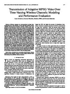
Fig. 5.

From (14), it is clear that the expected data rate for an AT is determined by the first state it enters the system. It is to be noted that the data rates are valid if the session time is finite. For sufficiently long session durations, ATs will experience all

11

Expected data rate at pedestrian speed

2500 analysis simulation

(13)

For the expected data rate corresponding to the initial state of the AT, we write the equation array as  R1 = p1,1 T1 + p1,2 R2     .. .   = ..  . = pi,i Ti + pi,i−1 Ri−1 + pi,i+1 Ri+1 Ri (14)   . .  ..   = ..   R11 = p11,11 T11 + p11,10 R10

10

Initial state

2000

Data rate (kbps)

µ1 Packet Data Network

data rates and they would tend to get the same expected data rate. However, for limited time duration, the data rate an AT perceives is highly influenced by its initial state. To investigate the nature of equations in (14), we set dk = 5 miles, α = 2. We plug (11) into (14), and use Simpson quadrature method to solve the integration numerically. We show the effect of AT’s speed and initial states on the expected data rate it gets. The compared speeds are pedestrian speed (4.5 mph) and vehicular speed (67.5 mph), and the decision cycle is set to be 1.67 seconds. Analytical results show slight differences from the feasible data rate T (shown in Table I) especially for 5, 6 and 7. To verify the results from our analytical model, we conducted simulation experiments with random movement of ATs. In our simulation, the AT’s starting position in the cell is uniformly distributed; it moves at a Gaussian random speed of N (0, rv2 /3) with uniformly distributed directions. We allow it to move freely in the cell for 30-60 minutes, however, we do not allow it to move out of the cell by restricting its maximum distance away from the BS to be less than dk . For the steady state results obtained, we calculate t/he expected data rate for each of the initial state i. Figures (5) and (6) show the analytical and simulation results for the aforementioned speeds with respect to the initial state (starting position) of ATs.

Data rate (kbps)

IV. E ND - TO - END P ERFORMANCE A NALYSIS

1500

1000

500

0

1

2

3

4

5

6

7

8

9

10

Initial state

Fig. 6.

Expected data rate at vehicular speed

11

This full text paper was peer reviewed at the direction of IEEE Communications Society subject matter experts for publication in the ICC 2007 proceedings.

B. Delay Variability

7000

For each data rate, service rate µi is the rate at which packets are served from the queue. The expected service rate is E[µi ] = Ri .

λV AR(1/µ) , Tq = 2(1 − λ/E[µ])

τ+

λσ 2 2(1−λ/Ri )

,

(18)

where λ can be regarded as the root of the quadratic equation (σ 2 −

2τ 2 )λ + (2W S/Ri + 2τ )λ − 2W S = 0, Ri

(19)

and the variables should satisfy the constraint (2W S/Ri + 2τ )2 + 8W S(σ 2 − 2τ /Ri ) ≥ 0.

RTT(ms)

3000

2000

1000

0

1

2

3

(16)

We assume that the window size of the TCP session be W S. To be precise, it can be an expected or average value over a period of data communication. Thus, λ can be approximated WS as λ = RT T . Combining equations (15) and (17), we get WS

4000

4

5

6

7

8

9

10

11

State

where λ is the rate at which RLP frames enter the queue, and V AR(1/µ) is the variance of service time. We denote that V AR(1/µ) = V AR(1/Ri ) = σ 2 . The round trip time (RTT) is an important parameter which determines the TCP throughput. We assume that the RTT is composed of two components – the delay in the backbone network, τ , and the queuing delay Tq . Thus, for each given initial state, (17) RT T = τ + Tq .

λ=

5000

(15)

The queuing can be modeled as an M/G/1 system, where the packets arrive according to a Poisson process with an arrival rate of λ. The service time differs with various channel conditions, and different wireless network behaviors, like MAC retransmission, so the service process is assumed as general. With this model, the queuing delay is given by PollaczekKhinchin equation as:

pedestrian speed, WS=16MSS vehicular speed, WS=16MSS pedestrian speed, WS=64MSS vehicular speed, WS=64MSS

6000

(20)

In any queuing system, if arrival rate (λ) is more than the service rate (µ) then the system is regarded as unstable. Thus, for our system, the only stable root is  S S 2τ 2 2 −( 2W ( 2W Ri + 2τ ) + Ri + 2τ ) + 8W Sσ − Ri λ= . 2τ 2(σ 2 − R ) i (21) To illustrate how RT T is related to the service or data rate (Ri ), and TCP window size (W S), we present the variance of RT T in Figure 7. We choose τ = 200ms as the backbone network delay. Also, we set M SS as the maximum segment size, which is typically 536 bytes in TCP/IP domain [10]. Plots show that when the AT is further from the BS, it would experience much larger RT T than near ones. The TCP window size decides the Bandwidth-Delay Product (BDP), and directly determines the expected RT T . We also observe that the RT T for slow moving ATs are slightly larger.

Fig. 7.

Round trip time

C. TCP Throughput Let us analyze the average TCP throughput achieved by an HDR system considering that each AT can only be in one of the modes (as shown in the Table I) at any point of time. We will assume that the TCP throughput is given by [9] M SS Wmax √ √ 3ap , ), 2 RT T RT T 2ap +T min(1,3 0 3 8 )p(1+32p ) (22) where, Wmax is the maximum supported TCP window size. RT T is the round trip time for the TCP acknowledgments. p is the segment loss probability, T0 is the TCP retransmission timer. a is a system constant describing the window increment rate, and we set it to be one. T0 is evaluated as an exponentially moving average of the instantaneous RT T s. If the TCP segment size is large, due to the lossy channel, the p is larger than small segments. If the bit error rate is b, then p for a K bits long segment is S = min(

K

p = 1 − (1 − b) .

(23)

If the TCP segment is fragmented into equal sized RLP frames, then the number of RLP frames obtained from a TCP segment would be N =  K R , where R is the size of RLP frames in bits. The RLP frame error loss probability, RLPloss , is therefore R

RLPloss = 1 − (1 − b) .

(24)

For a TCP segment to be reassembled successfully, all the N frames must be received correctly. If one or more RLP frames fail, the TCP segment is lost. Thus, the TCP segment loss probability, p, is given by N

p = 1 − (1 − RLPloss ) .

(25)

In Figure 8, we try to capture the impact of BER, AT’s velocity and TCP segment size. Compared with 128-bit segmentation, we find 64 bits per segment helps to improve TCP throughput by 20%. Also, slow moving AT gains another 2% throughput than fast moving ones. It might be noted that due to fading, fast moving AT will eventually get worse TCP throughput performance. We finally present the TCP throughput for HDR system for each initial state in Figure 9. We set p = 0.1% and normalize

This full text paper was peer reviewed at the direction of IEEE Communications Society subject matter experts for publication in the ICC 2007 proceedings.

R EFERENCES

Normalized TCP throughput

100% vehicular speed 64bits/seg pedestrian speed 64bits/seg pedestrian speed 128bits/seg vehicular speed 128bits/seg

94%

88%

82%

76%

70% −5 10

−4

−3

10

Fig. 8.

10

BER TCP throughput Vs. BER

Normalized TCP throughput

100% vehicular speed WS=128MSS vehicular speed WS=32MSS pedestrian speed WS=128MSS pedestrian speed WS=32MSS

80%

60%

[1] http://www.3gpp2.org [2] Y. Bai, P. Zhu, A. Rudrapatna, A. T. Ogielski, “Performance of TCP/IP over IS- 2000 based CDMA radio links”, Proc. IEEE 52th VTC’2000Fall, 2000, pp. 1036-1040. [3] Y. Bai, A. T. Ogielski. “TCP over asymmetric CDMA radio links”, Proc. IEEE 52th VTC’2000-Fall, 2000, pp. 1015-1018. [4] P. Bender, P. Black, M. Grob, R. Padovani, N. Sindhushyana, and A. Viterbi, “CDMA/HDR: a bandwidth efficient high speed wireless data service for nomadic users”, IEEE Communications Magazine, Volume: 38 Issue: 7, July 2000, pp. 70-77. [5] T. Bonald and A. Proutiere, “Wireless Downlink Data Channels: User Performance and Cell Dimensioning”, ACM Mobicom, 03, pp. 339-352. [6] A. S. Joshi, M. N. Umesh, A. Kumar, T. Mukhopadhyay, K. Natesh, S. Sen, A. Arunachalam, “Performance evaluation of TCP over radio link protocol in TIA/EIA/IS-99 environment”, ICPWC 1999, pp. 216-220. [7] F. Khan, S. Kumar, K. Medepalli, S. Nanda, “TCP performance over cdma2000 RLP”, Proc. IEEE 51st VTC’2000-Spring, pp. 41-45. [8] H. Lin and S.K. Das, “Performance Study of Link Layer and MAC Layer Protocols in supporting TCP in 3G CDMA Systems,” To appear in IEEE Transactions on Mobile Computing. [9] J. Padhye, V. Firoiu, D. Towsley and J. Kurose, “Modeling TCP Throughput: A Simple Model and its Empirical Validation”, Proc. ACM SIGCOMM 1998, pp. 303-314. [10] J. Postel, RFC 879, http://www.ietf.org/rfc/rfc879 [11] H. M. Syed, K. Das and M. Devetsikiotis, “TCP performance and buffer provisioning for Internet in wireless networks, MASCOTS 99, pp. 48-55. [12] G. Wu, Y. Bai, J. Lai, A. Ogielski, “Interactions between TCP and RLP in wireless Internet”, Proc. IEEE GlobeCom 1999, pp. 661-666.

A PPENDIX Refer toFigure 2. O is of the radius of state i−1, and the Saebf radius of d is rv . The probability of qi,i−1 is qi,i−1 = πr 2 

40%

v

20%

0

1

2

3

4

5

6

7

8

9

10

11

State Fig. 9.

TCP throughput for HDR system

the maximum values to one. Again, we find that slow moving AT gain more throughput, and larger TCP window size helps improve throughput. Since TCP transmission cannot exceed its buffer size (i.e., TCP window size), small W S value limits the TCP throughput. However, if the TCP window is large enough to buffer all the data (i.e., larger than BDP), the system will not achieve better throughput either. We also find that the proper TCP window size for HDR system is 64 MSS and that matches the maximum BDP. V. C ONCLUSIONS Multi-rate cellular networks introduce diverse data rates into the last hop communication and enable the system to exploit the best data rate for users given their SINR. We propose a Markovian model to calculate how frequently users change their data rate. Based on this model, we further obtain the expected data rate for user with different initial states. To validate our model, we conduct extensive simulations. We also use an M/G/1 queuing model to find how TCP throughput changes with window size, data rate, and loss rate. Numerical results, that are in accord with simulation results, illustrate that smaller link layer segments, less BER, and slower movement help improve TCP throughput. We also propose the practical TCP window size for HDR system.

SaOd

Saebf = S
+ S
− SOadb af b aeb = SOadb /2 = s(s − ri−1 )(s − rv )(s − x)

ri−1 +rv +x 2 √. Let h be the height 2 s(s−ri−1 )(s−rv )(s−x) can easily get h = x  aOb h 2 2 S
= 2π πri−1 = arcsin ( ri−1 )ri−1 af b   adb for d, S
= 2π πrv2 = arcsin ( rhv )rv2 aeb

where s =

qi,i−1 =

of aOd, and we  for O, Thus, we get

1 h h 2 [arcsin ( )ri−1 + arcsin ( )rv2 2 πrv r rv i−1 −2 s(s − ri−1 )(s − rv )(s − x)]

Refer to Figure 3. The probability of qi,i+1 is qi,i+1 = Therefore, SXwyz = S
+ SXOyd − S
Xwy Xzy SOdX = SXOyd /2 = s∗ (s∗ − ri )(s∗ − rv )(s∗ − x)

SXwyz πrv2 .

where s∗ = ri +r2v +x . Let k be the height of XOd, and we also can get 2 s∗ (s∗ − ri )(s∗ − rv )(s∗ − x) k= x   yOy 2
for O, S = 2π πri = arcsin ( rki )ri2 Xzy   k 2 2 for d, S
= Xdy 2π πrv = arcsin ( rv )rv Therefore, Xwy

qi,i+1 =

1 k k [arcsin ( )rv2 − arcsin ( )ri2 2 πrv rv ri +2 s∗ (s∗ − ri )(s∗ − rv )(s∗ − x)]