Performance of an MPI-only Semiconductor Device Simulator on a

SANDIA REPORT SAND2009-0179 Unlimited Release Printed January 2009

Performance of an MPI-only Semiconductor Device Simulator on a Quad Socket/Quad Core InfiniBand Platform Paul T. Lin, John N. Shadid Prepared by Sandia National Laboratories Albuquerque, New Mexico 87185 and Livermore, California 94550 Sandia is a multiprogram laboratory operated by Sandia Corporation, a Lockheed Martin Company, for the United States Department of Energy’s National Nuclear Security Administration under Contract DE-AC04-94-AL85000. Approved for public release; further dissemination unlimited.

Issued by Sandia National Laboratories, operated for the United States Department of Energy by Sandia Corporation. NOTICE: This report was prepared as an account of work sponsored by an agency of the United States Government. Neither the United States Government, nor any agency thereof, nor any of their employees, nor any of their contractors, subcontractors, or their employees, make any warranty, express or implied, or assume any legal liability or responsibility for the accuracy, completeness, or usefulness of any information, apparatus, product, or process disclosed, or represent that its use would not infringe privately owned rights. Reference herein to any specific commercial product, process, or service by trade name, trademark, manufacturer, or otherwise, does not necessarily constitute or imply its endorsement, recommendation, or favoring by the United States Government, any agency thereof, or any of their contractors or subcontractors. The views and opinions expressed herein do not necessarily state or reflect those of the United States Government, any agency thereof, or any of their contractors. Printed in the United States of America. This report has been reproduced directly from the best available copy. Available to DOE and DOE contractors from U.S. Department of Energy Office of Scientific and Technical Information P.O. Box 62 Oak Ridge, TN 37831 Telephone: Facsimile: E-Mail: Online ordering:

(865) 576-8401 (865) 576-5728 [email protected] http://www.osti.gov/bridge

Available to the public from U.S. Department of Commerce National Technical Information Service 5285 Port Royal Rd Springfield, VA 22161 (800) 553-6847 (703) 605-6900 [email protected] http://www.ntis.gov/help/ordermethods.asp?loc=7-4-0#online

NT OF E ME N RT

GY ER

•

U NIT

IC A

•

ED

ST

ER

DEP A

Telephone: Facsimile: E-Mail: Online ordering:

A TES OF A

M

2

SAND2009-0179 Unlimited Release Printed January 2009

Performance of an MPI-only Semiconductor Device Simulator on a Quad Socket/Quad Core InfiniBand Platform Paul T. Lin, John N. Shadid Electrical and Microsystem Modeling Department Sandia National Laboratories P.O. Box 5800 Mail Stop 0316 Albuquerque, NM 87185-0316 email contact: [email protected]

Abstract This preliminary study considers the scaling and performance of a finite element (FE) semiconductor device simulator on a capacity cluster with 272 compute nodes based on a homogeneous multicore node architecture utilizing 16 cores. The inter-node communication backbone for this Tri-Lab Linux Capacity Cluster (TLCC) machine is comprised of an InfiniBand interconnect. The nonuniform memory access (NUMA) nodes consist of 2.2 GHz quad socket/quad core AMD Opteron processors. The performance results for this study are obtained with a FE semiconductor device simulation code (Charon) that is based on a fully-coupled Newton-Krylov solver with domain decomposition and multilevel preconditioners. Scaling and multicore performance results are presented for large-scale problems of 100+ million unknowns on up to 4096 cores. A parallel scaling comparison is also presented with the Cray XT3/4 Red Storm capability platform. The results indicate that an MPI-only programming model for utilizing the multicore nodes is reasonably efficient on all 16 cores per compute node. However, the results also indicated that the multilevel preconditioner, which is critical for large-scale capability type simulations, scales better on the Red Storm machine than the TLCC machine.

3

Acknowledgment The first author is very grateful to Jeffrey Ogden for numerous helpful discussions concerning the TLCC machine. He is grateful to Sophia Corwell for her help and thanks Marcus Epperson, Jesse Livesay and the rest of the TLCC team. He thanks Suzanne Kelly, Robert Ballance, Michael Davis and the rest of the Red Storm team for their help. He also thanks Brian Barrett, Tommy Minyard, Gary Hennigan, and Michael Heroux for helpful discussion. The authors are very grateful for the generous support from the DOE NNSA ASC program, DOE Office of Science, and DOE ASCR IAA.

4

Contents 1 Introduction . . . . . . . . . . . . . . . . . . . . . . . . . . . . . . . . . . . . . . . . . . . . . . . . . . . . . . . . . . . . . . . . . . . . . 2 A Brief Description of the FE Semiconductor Model . . . . . . . . . . . . . . . . . . . . . . . . . . . . . . 3 Scaling Results . . . . . . . . . . . . . . . . . . . . . . . . . . . . . . . . . . . . . . . . . . . . . . . . . . . . . . . . . . . . . . . . . . . 3.1 Weak scaling study up to 112 million unknowns . . . . . . . . . . . . . . . . . . . . . . . . 3.2 Weak scaling study up to 28 million unknowns . . . . . . . . . . . . . . . . . . . . . . . . . 3.3 Fixed problem size scaling study (28 million unknowns) . . . . . . . . . . . . . . . . . . 4 Multicore Results . . . . . . . . . . . . . . . . . . . . . . . . . . . . . . . . . . . . . . . . . . . . . . . . . . . . . . . . . . . . . . . . 4.1 Memory and placement of MPI tasks on cores . . . . . . . . . . . . . . . . . . . . . . . . . . 4.2 Scaling for a single compute node . . . . . . . . . . . . . . . . . . . . . . . . . . . . . . . . . . . . 4.3 Effects of network and compute nodes on scaling . . . . . . . . . . . . . . . . . . . . . . . 5 Conclusions . . . . . . . . . . . . . . . . . . . . . . . . . . . . . . . . . . . . . . . . . . . . . . . . . . . . . . . . . . . . . . . . . . . . . . References . . . . . . . . . . . . . . . . . . . . . . . . . . . . . . . . . . . . . . . . . . . . . . . . . . . . . . . . . . . . . . . . . . . . . . . . . . .

5

9 11 13 14 16 19 23 23 25 27 29 30

Figures 1 2 3 4 5 6 7

(a) Signed logarithm of doping for 2×1.5µm 2D NPN BJT; (b) Corresponding steady-state electric potential for 2 × 1.5µm 2D NPN BJT at 0.3V bias . . . . Weak scaling study up to 112 million unknowns . . . . . . . . . . . . . . . . . . . . . . . . Weak scaling study up to 112 million unknowns: ratio of times TLCC/RS . . . Weak scaling study up to 28 million unknowns . . . . . . . . . . . . . . . . . . . . . . . . . Weak scaling study up to 28 million unknowns: ratio of times TLCC/RS . . . . Fixed problem size scaling study with 28 million unknowns . . . . . . . . . . . . . . . Fixed problem size scaling study with 28 million unknowns: ratio of times TLCC/RS . . . . . . . . . . . . . . . . . . . . . . . . . . . . . . . . . . . . . . . . . . . . . . . . . . . . . . .

6

13 16 18 19 21 22 22

Tables 1 2 3 4 5 6 7 8 9 10 11

Weak scaling study up to 112 million unknowns comparing one-level preconditioner for TLCC (MVAPICH) and Red Storm. . . . . . . . . . . . . . . . . . . . . . . . . Weak scaling study up to 112 million unknowns comparing three-level preconditioner for TLCC (MVAPICH) and Red Storm. . . . . . . . . . . . . . . . . . . . . . Weak scaling study up to 28 million unknowns comparing one-level preconditioner for TLCC (MVAPICH) and Red Storm. . . . . . . . . . . . . . . . . . . . . . . . . . Weak scaling study up to 28 million unknowns comparing three-level preconditioner for TLCC (MVAPICH) and Red Storm. . . . . . . . . . . . . . . . . . . . . . . . . Fixed problem size scaling study with 28 million unknowns comparing onelevel preconditioner for TLCC (MVAPICH) and Red Storm. . . . . . . . . . . . . . . Fixed problem size scaling study with 28 million unknowns comparing threelevel preconditioner for TLCC (MVAPICH) and Red Storm. . . . . . . . . . . . . . . Effect on performance due to local vs. nonlocal memory access on a node. . . . Strong scaling on single node: one-level ILU (“speedup” is abbreviated as “s.u.”). . . . . . . . . . . . . . . . . . . . . . . . . . . . . . . . . . . . . . . . . . . . . . . . . . . . . . . . . . Strong scaling on single node: multigrid preconditioner; “speedup” is abbreviated as “s.u.” . . . . . . . . . . . . . . . . . . . . . . . . . . . . . . . . . . . . . . . . . . . . . . . . . . . Weak scaling on single node: 110K DOF/core one-level ILU . . . . . . . . . . . . . . Multicore network/node study starting with 256 compute nodes. . . . . . . . . . .

7

14 15 17 17 20 20 24 25 26 27 27

8

1

Introduction

A current pathway to increase the peak performance of the next generation supercomputers is to utilize large numbers of powerful compute nodes comprised of multiple sockets with multiple cores on each socket. It has been forecasted that by about 2020 compute nodes will have a thousand cores [25]. This is a significant cause of concern for numerical methods and scientific application software developers who have typically had the performance of their codes limited by the bandwidth from the compute processor to local memory. Although there appears to be a belief that the single-level MPI-only programming model should be sufficient for the next 3-5 years, there appears to be no general consensus on the most effective programming model for larger core count multicore nodes [9]. This preliminary study considers the performance of an existing semiconductor device simulation code (Charon) to begin to elucidate a number of important issues in utilizing multicore architecture nodes. An example of the trend to multicore nodes is the recent arrival of the Tri-Laboratory Linux Capacity Clusters (TLCC) at Sandia National Labs (SNL). Sandia, Los Alamos, and Lawrence Livermore national laboratories have collaborated to purchase the same high performance capacity linux clusters, the TLCC [2]. Sandia is receiving three machines: two for New Mexico and one for California. Very briefly the SNL TLCC machine has the following characteristics1 : • 38 TFlops peak • 272 compute nodes (total of 4352 cores) – quad socket 2.2 GHz AMD Opteron (Barcelona) quad core processors – Memory: 32 GB DDR2 RAM per node • Interconnect – Interconnect: InfiniBand with OFED software stack – InfiniBand card: Mellanox ConnectX HCA • Software environment – RedHat Enterprise Linux on compute nodes – Open MPI and MVAPICH with Intel, PGI, GNU, and Pathscale compilers Although the TLCC machines are intended to be capacity machines, it is important to understand how well applications codes will scale on a multinode machine with a commodity interconnect such as InfiniBand. As a point of comparison this study will consider the relative performance of the TLCC machine with the Cray XT3/4. The Cray XT3/4 (Red Storm) 1

Summary from the TLCC web site (https://computing.sandia.gov/platforms/tlcc)

9

has a custom designed interconnect that maximizes performance and scalability and employs both dual and quad core nodes. The limited scope of this study is to examine the performance of a state of the art C++ object oriented transport reaction code, Charon, on the TLCC machine. The Charon code was originally developed to model semiconductor devices via the drift-diffusion equations, but it can also model magnetohydrodynamics (MHD). This study considers the performance of Charon for solving a steady-state drift-diffusion problem, and is not intended to be exhaustive. The authors make no claims about how other physics codes will perform. Charon simulations will be run on TLCC to examine two issues: how does the scalability of a commodity interconnect compare with the custom high performance interconnect on Red Storm and how efficiently can the 16 cores on the compute node be utilized. These studies were performed on the first SNL TLCC machine, named “Unity.” In this study, two different implementations of MPI are used on the TLCC Unity machine. The first is Open MPI 1.2.7 with the Intel 10.1 compiler. The second implementation is MVAPICH 1.0.1 with the Intel 10.1 compiler. Two different implementations of MPI were evaluated because in an initial study the Open MPI scaling of Charon was found to be extremely poor on 4096 cores of TLCC compared with 4096 cores of Red Storm. Based on the results of Minyard’s[15] experience with the Texas Advanced Computing Center (TACC) Ranger machine the decision to include an alternate MPI implementation other than Open MPI was made. The TACC team found that an alternate MPI implementation, MVAPICH (developed at Ohio State University), was scaling considerably better than Open MPI. Although the TACC Ranger team’s Open MPI scaling issue was in startup time, and our Open MPI scaling issue is occurring during run-time and therefore is most likely a different issue, the fact that MVAPICH was scaling better for the TACC team led us to try MVAPICH for Charon. In our studies we found that Charon implemented with MVAPICH scaled considerably better with Open MPI, as the results that follow demonstrate.

10

2

A Brief Description of the FE Semiconductor Model

The Charon semiconductor device modeling code solves the drift-diffusion equations [13, 26]: ∇ · (²E) − q (p − n + C) = 0, ∂n q − ∇ · Jn + qG = 0, ∂t ∂p + ∇ · Jp + qG = 0, q ∂t

(1) (2) (3)

where E = −∇ψ, Jn = qnµn E + qDn ∇n, Jp = qpµp E − qDp ∇p. The unknowns are: ψ, the electrostatic potential, n, the electron concentration (number of electrons per volume), and p, the hole concentration (number of holes per volume). The parameters for the model include, ², the permittivity of the semiconductor material, q, the fundamental electron charge, µn and µp , the electron and hole mobilities, respectively, and Dn and Dp , the electron and hole diffusion coefficients, respectively. The electrostatic potential source term C is the doping profile, and G is the generation/recombination source term in the electron and hole balance equations. For the test case considered in this paper, the generation/recombination source term is negligible. These equations are discretized using a stabilized finite element formulation [20]. This discretization is associated with a simple extension of an SUPG-type approach to the driftdiffusion system. The methodology is based on a variation of the streamline upwind PetrovGalerkin (SUPG) type FE formulations of Hughes et. al. [10, 11] and Shakib [24]. Discretization of the drift-diffusion equations produces a large sparse, strongly coupled nonlinear system. This system is solved via a Newton-Krylov algorithm [1, 21], where the linear systems (generated at each Newton step) are solved using a Krylov accelerator [16, 5]. The choice of the preconditioner is critical to the performance of the linear solver. The two main preconditioners considered in this study are a one-level domain decomposition (DD), with a subdomain solver based on an incomplete lower/upper (ILU) factorization, and an algebraic multilevel type preconditioner. The multigrid preconditioner is a Petrov-Galerkin smoothed aggregation approach for nonsymmetric linear systems [19]. More information on these details of these methods and representative results for large-scale performance of various finite element applications can be found in [23, 22, 18, 14]. Briefly, in terms of software, the initial load-balance and fine-level nonoverlapping subdomains are obtained using Chaco [6]. The Trilinos package, IFPACK, provides incomplete factorizations [17]. Krylov methods are implemented in AztecOO [27, 7]. A sparse KLU 11

factorization is used for the coarse direct solver [3]. The multigrid cycles and grid transfers are provided by ML [4]. ML also provides aggregation routines though METIS and ParMETIS [12] that are used in this paper. Access to this software is obtained via the Trilinos framework [8].

12

3

Scaling Results

The numerical studies involve the steady-state solution of the two-dimensional drift-diffusion equations for a 2 × 1.5µm silicon NPN bipolar junction transistor (BJT) (Figure 1). Briefly,

(a) BJT doping

(b) BJT electric potential

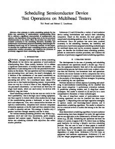
Figure 1. (a) Signed logarithm of doping for 2 × 1.5µm 2D NPN BJT; (b) Corresponding steady-state electric potential for 2 × 1.5µm 2D NPN BJT at 0.3V bias

“NPN” denotes a transistor with n-type (material with additional negative charge carriers), p-type (material with excess holes), and n-type material. This geometry has three contacts. The base at the top left corner, the emitter at the top right corner, and the collector along the entire bottom. Both the emitter and base are 0.1µm wide. The steady-state calculation is performed with a voltage bias of 0.3V: the base and collector are held at ground and the emitter is assigned a voltage of -0.3V. The initial guess for the drift-diffusion equations is taken as the solution to the nonlinear poisson (NLP) problem [20]. Figure 1a shows the signed logarithm of the doping for the device. The signed logarithm slog(x) is defined as slog(x) = sign(x)log10 (1 + |x|). Note that the doping, C, varies between 1019 and −1016 (N-doping is positive). Figure 1b shows the corresponding steady-state electric potential solution. In this section, TLCC results will be compared with Red Storm results. The TLCC results in this section use all 16 cores per compute node. The Red Storm results in this section use the older 2.4 GHz dual core nodes (both cores per compute node). Charon was built on Red Storm using the PGI 6.2.5 build environment. It is of interested to compare the performance of a one-level preconditioner and a multigrid preconditioner on the two platforms (TLCC and Red Storm) as the communication pattern is significantly different. The one-level DD ILU preconditioner involves subdomain boundary data exchange with its nearest neighbors. The multigrid preconditioner uses this same DD ILU preconditioner as smoothers on the fine and medium mesh and KLU direct solver on the coarse mesh. So not only does the multigrid preconditioner require boundary data exchange 13

proc

fine grid unk

16 438K 64 1.75M 256 6.98M 1024 27.9M 4096 112M

iter/ Newt 142 287 571 1145 2267

1-level DD ILU(2) overlap=1 TLCC (MVAPICH) Red Storm Time/Newton step (sec) iter/ Time/Newton step prec linear Jac Newt Newt prec linear Jac 0.88 13.9 2.88 18.0 142 0.94 8.44 7.00 0.91 44.2 2.93 48.4 287 0.96 24.9 7.00 0.95 157 2.96 161 571 0.99 84.1 7.14 1.00 640 3.01 644 1145 1.02 317 7.57 1.05 2441 3.13 2447 2264 1.05 1192 7.86

(sec) Newt 17.9 34.3 93.9 327 1202

Table 1. Weak scaling study up to 112 million unknowns comparing one-level preconditioner for TLCC (MVAPICH) and Red Storm.

with its nearest neighbors for ILU on the fine and medium mesh, it also requires more complex communication for the grid transfer operators and the coarse mesh solve. Below the weak scaling for two different problem sizes per core (27,000 and 6800) illustrate the relative performance of the two machines.

3.1

Weak scaling study up to 112 million unknowns

A weak scaling study was performed on TLCC for both a one-level DD ILU preconditioner and a three-level multigrid preconditioner, using both the Open MPI and MVAPICH built executables. The problem was scaled up to 112 million unknowns on 4096 cores (27,000 unknowns per core). The results for the one-level preconditioner on TLCC with Charon built with MVAPICH are presented in Table 1 and compared with the same scaling study performed on Red Storm. Under “Time/Newton step”, “prec” denotes the time per Newton step to construct the preconditioner, “linear” denotes the time to perform the linear solve (this includes the time to construct the preconditioner), “Jac” denotes the time to construct the Jacobian, and “Newt” denotes the total time to perform everything in a Newton step (includes linear solve and time to construct the Jacobian). For the 4096 core case, 256 compute nodes on TLCC are used while 2048 compute nodes on Red Storm are used. Note that entry for the 4096-core TLCC MVAPICH one-level preconditioner case is an estimate because the calculation crashed during the sixth Newton step (calculation would have taken seven Newton steps) when one of the compute nodes failed. However, a 4096-core TLCC Open MPI calculation was completed earlier, and careful comparison between the MVAPICH and Open MPI calculation showed that the former was 16% faster, so the estimate in the table is an accurate estimate. The results for the three-level preconditioner are presented in Table 2, where the TLCC results are for Charon with MVAPICH. The three-level PetrovGalerkin multigrid preconditioner uses a W(1,1) cycle with coarser levels generated using METIS/ParMETIS and 125 nodes per aggregate. 14

proc

fine grid unk

16 438K 64 1.75M 256 6.98M 1024 27.9M 4096 112M

iter/ Newt 48 70 95 125 152

3-level PG-SA W(1,1) agg125 TLCC (MVAPICH) Red Storm Time/Newton step (sec) iter/ Time/Newton step prec linear Jac Newt Newt prec linear Jac 1.50 6.22 2.89 10.2 49 1.94 5.16 6.86 1.68 9.38 2.94 13.4 72 2.10 7.40 6.86 2.16 14.9 2.95 19.0 97 2.54 11.3 7.00 3.38 29.0 3.02 33.2 125 2.89 16.8 7.71 10.4 74.5 3.15 78.9 153 4.47 25.7 7.00

(sec) Newt 14.6 19.1 21.0 27.3 35.4

Table 2. Weak scaling study up to 112 million unknowns comparing three-level preconditioner for TLCC (MVAPICH) and Red Storm.

The comparison between TLCC and Red Storm for the one-level and three-level preconditioners are plotted in Figure 2(a) and 2(b) respectively. The time plotted on the vertical axes is the CPU time per Newton step in seconds. Although the results for TLCC for Charon built with Open MPI were not presented in the tables, they are included in the plots. From the tables and figures a few issues should be pointed out to interpret the results. First the one-level DD ILU preconditioner, in general, scales very poorly. This is apparent from the iteration count that increases significantly with problem size (and core count) in Table 1. This accounts for the significant increase in CPU time in Figure 2(a) and is in contrast to the three-level method in Figure 2(b) (note the change in CPU time magnitudes). This scaling illustrates why some type of multilevel technique is required to approach truly scalable simulation methods and therefore modern large-scale computing platforms need to run these methods efficiently. In Figure 2 the increase in CPU times for the simulation have contributions from the increase in the number of iterations (an algorithmic issue) and in the inefficiency of the platform scaling (most likely due to network scaling). To attempt to more clearly show the effect of the scaling efficiency of the network, a plot of the ratio of the TLCC time (Charon with MVAPICH) over the Red Storm time is presented in Figure 3 for the two different preconditioners. For the 1024 core case, as an example, for the one-level preconditioner this ratio is approximately 2, which means that the TLCC calculation took twice as long as the Red Storm calculation. The horizontal dashed green and black lines are included to denote the case where the TLCC and Red Storm are scaling in a similar fashion for the one-level and three-level preconditioners. The fact that the ratio of TLCC over Red Storm time is growing, as the problem size (and core count), is scaled indicates that the TLCC network does not scale as well as the interconnect on Red Storm. Further the TLCC performance on the multilevel algorithm deteriorates at a faster rate due to the increased communication required for the coarser levels and transfers between levels. In terms of the choice of MPI implementation on TLCC, Open MPI or MVAPICH, for the one-level preconditioner it does not matter until more than 1000 cores are used. 15

Weak Scaling Study: 1-level DD ILU Scaled to 112 Million DOF

2500

2000

TLCC Open MPI 1.2.7 OFED 1.2 TLCC MVAPICH 1.0.1 OFED 1.2 Red Storm

100

TLCC 2.2 GHz Quad Socket/Quad Core Red Storm 2.4 GHz Dual Core

ILU(2) overlap=1

1500

4096c

1000

1024c

500

0 5 10

64c

16c

10

6

256c

Charon Steady Drift-Diffusion 2x1.5 um BJT 0.3V

4096c

CPU Time per Newton Step (sec)

CPU Time per Newton Step (sec)

3000

Weak Scaling Study: 3-level PG-SA ML Scaled to 112 Million DOF

Charon Steady Drift-Diffusion 2x1.5 um BJT 0.3V

80

60

TLCC Open MPI 1.2.7 OFED 1.2 TLCC MVAPICH 1.0.1 OFED 1.2 Red Storm

4096c

TLCC 2.2 GHz Quad Socket/Quad Core Red Storm 2.4 GHz Dual Core

ML 3-level PG-SA W(1,1) agg125 1024c

40 4096c

20

64c

256c

1024c

16c

1024c

10

7

Unknowns

10

0 5 10

8

(a) 1-level DD ILU

10

6

10

7

Unknowns

10

8

(b) 3-level W(1,1) agg125

Figure 2. Weak scaling study up to 112 million unknowns

At 4096 cores, Charon with MVAPICH is 16% faster than Open MPI. For the three-level preconditioner, for more than 256 cores MVAPICH is scaling better than Open MPI, and Charon with Open MPI is 50% slower than with MVAPICH for 1024 cores. Not only does Open MPI scale worse, it appears to have a possible robustness issue as the 4096 core case with the three-level preconditioner failed due to an InfiniBand stack resource issue while MVAPICH did not seem to have any problems. Finally, one can observe that the two curves in Figure 2(b) cross. This is because the time to construct the Jacobian and preconditioner is considerably higher for Red Storm than on the TLCC machine. For smaller problems, the time to construct the preconditioner is greater than the linear solve time on Red Storm. At larger problem sizes (core counts) the time to solve the linear system dominates and the effectiveness of the scaling of the network as described above becomes more critical to the overall solution time.

3.2

Weak scaling study up to 28 million unknowns

The previous weak scaling study does not give the complete picture how Open MPI and MVAPICH on TLCC compare at 4096 cores for the multigrid preconditioner. A second weak scaling study was performed, but with a quarter the number of unknowns as the previous problem. As with the previous study, this study was performed on TLCC for both a onelevel DD ILU preconditioner and a three-level multigrid preconditioner for Charon built with both Open MPI and MVAPICH. The problem was scaled up to 28 million unknowns on 4096 cores (6800 unknowns per core). The results for the one-level and three-level preconditioner 16

proc

fine grid unk

16 110K 64 438K 256 1.75M 1024 6.98M 4096 27.9M

iter/ Newt 76 157 310 614 1244

1-level DD ILU(2) overlap=1 TLCC (MVAPICH) Red Storm Time/Newton step (sec) iter/ Time/Newton step prec linear Jac Newt Newt prec linear Jac 0.23 1.43 0.72 2.46 76 0.26 1.04 1.86 0.24 4.19 0.74 5.24 157 0.27 2.68 1.43 0.26 13.2 0.75 14.3 310 0.28 7.69 1.71 0.29 47.8 0.76 48.9 614 0.30 25.9 1.79 0.36 193 0.77 195 1244 0.32 97.6 1.57

(sec) Newt 3.71 5.43 10.3 28.4 100

Table 3. Weak scaling study up to 28 million unknowns comparing one-level preconditioner for TLCC (MVAPICH) and Red Storm.

proc

fine grid unk

16 110K 64 438K 256 1.75M 1024 6.98M 4096 27.9M

iter/ Newt 33 55 80 114 153

3-level PG-SA W(1,1) agg125 TLCC (MVAPICH) Red Storm Time/Newton step (sec) iter/ Time/Newton step prec linear Jac Newt Newt prec linear Jac 0.40 1.19 0.72 2.20 33 0.83 1.45 1.71 0.45 1.97 0.74 3.00 55 0.89 2.12 1.71 0.66 3.77 0.76 4.83 80 1.08 3.57 1.71 1.84 12.0 0.76 13.0 115 1.91 9.77 1.79 5.97 50.2 0.79 51.4 151 3.35 19.2 1.86

Table 4. Weak scaling study up to 28 million unknowns comparing three-level preconditioner for TLCC (MVAPICH) and Red Storm.

17

(sec) Newt 4.14 4.86 6.14 12.2 21.9

TLCC/(Red Storm) Time per Newton Step

Weak Scaling Study: Charon Steady Drift-Diffusion 2x1.5 um BJT 0.3V TLCC 2.2 GHz Quad Socket/Quad Core; Red Storm 2.4 GHz Dual Core 3

1-level DD ILU 3-level PG-SA W(1,1) agg125

2.5

4096c

2 1024c 256c

1.5 64p

1

64p

16p

1024c similar scaling

256c

similar scaling

0.5

0 5 10

10

6

10

Unknowns

7

10

8

Figure 3. Weak scaling study up to 112 million unknowns: ratio of times TLCC/RS

are presented in Table 3 and Table 4 respectively (for TLCC, only the results for Charon with MVAPICH are presented). All runs took seven Newton steps. The three-level PetrovGalerkin multigrid preconditioner uses a W(1,1) cycle with coarser levels generated using METIS/ParMETIS and 125 nodes per aggregate. The comparison between TLCC and Red Storm for the one-level and three-level preconditioners are plotted in Figure 4(a) and 4(b) respectively. The TLCC results for Charon built with Open MPI are also plotted. The time plotted on the vertical axes is the CPU time per Newton step in seconds. One can observe from Figure 4(b) that compared with Red Storm, the multigrid preconditioner on TLCC (MVAPICH) scales well up to 1024 cores, but not so well for the 4096 core case. For the three-level preconditioner, for the 4096-core case, Open MPI takes a factor of 2.6 as much time as MVAPICH, and a factor of 6 as much time as Red Storm. It is rather disconcerting that Open MPI is slower than MVAPICH by such a large margin, because typically when application developers test the scalability of their codes, they assume that lack of scalability is due to their code rather than possible lack of scalability of the MPI implementation. Figure 5 presents the ratio of the TLCC time (Charon with MVAPICH) over the Red Storm time. The horizontal dashed green and black lines would denote the case where TLCC and Red Storm were scaling in a similar manner for the one-level and three-level preconditioners respectively. The run time difference for the three-level preconditioner calculation on 4096 cores on TLCC than Red Storm was a factor of 2.4. Multigrid preconditioners are critical to obtain solutions of large scale simulations. This difference in performance shows that a high performance scalable network is important to large scale simulations. 18

Weak Scaling Study: 3-level PG-SA ML Scaled to 28 Million DOF

Weak Scaling Study: 1-level DD ILU Scaled to 28 Million DOF Charon Steady Drift-Diffusion 2x1.5 um BJT 0.3V TLCC Open MPI 1.2.7 OFED 1.2 TLCC MVAPICH 1.2.7 OFED 1.2 Red Storm

200

Charon Steady Drift-Diffusion 2x1.5 um BJT 0.3V

140 4096c

CPU Time per Newton Step (sec)

CPU Time per Newton Step (sec)

250

TLCC 2.2 GHz Quad Socket/Quad Core Red Storm 2.4 GHz Dual Core

ILU(2) overlap=1

150

4096c

100

1024c

50 16c

0 5 10

64c

256c

10

6

Unknowns

TLCC Open MPI 1.2.7 OFED 1.2 TLCC MVAPICH 1.0.1 OFED 1.2 Red Storm

120

TLCC 2.2 GHz Quad Socket/Quad Core Red Storm 2.4 GHz Dual Core

100

ML 3-level PG-SA W(1,1) agg125

80 60

4096c

40

10

10

0 5 10

8

(a) 1-level DD ILU

4096c

1024c

20 16c

7

4096c

256c

64c

10

6

Unknowns

10

7

10

8

(b) 3-level W(1,1) agg125

Figure 4. Weak scaling study up to 28 million unknowns

3.3

Fixed problem size scaling study (28 million unknowns)

A fixed problem size scaling study was performed on TLCC for both a one-level DD ILU preconditioner and a three-level multigrid preconditioner, for Charon with Open MPI and MVAPICH. A mesh with 28 million unknowns was used for all the cases as the number of cores was increased from 128 to 4096. The results for the one-level and three-level preconditioner are presented in Table 5 and 6 respectively, and compared with the same scaling study performed on Red Storm. Once again, the TLCC results for Charon with MVAPICH are presented in the tables while the TLCC results for Charon with Open MPI are not included in the tables. All runs took seven Newton steps. The three-level Petrov-Galerkin multigrid preconditioner uses a W(1,1) cycle with coarser levels generated using METIS/ParMETIS and 125 nodes per aggregate. The comparison between TLCC and Red Storm for the one-level and three-level preconditioners are plotted in Figure 6(a) and 6(b) respectively. Once again the TLCC results for Charon with Open MPI are also plotted in the figures. The considerably poorer scaling of Charon with Open MPI compared to MVAPICH on TLCC is apparent from the figures. Figure 7 presents the ratio of the TLCC time (Charon with MVAPICH) over the Red Storm time. In Figure 7, the horizontal dashed green and black lines would denote the case where TLCC and Red Storm were scaling in a similar manner for the one-level and three-level preconditioners respectively. From the figure, the performance of the three-level preconditioner on TLCC MVAPICH is the same as on Red Storm up to 512 cores and competitive up to 2048 cores. The situation deteriorates at 3072 cores, and at 4096 cores the difference is a factor of 2.4. It is clear that beyond 2048 cores the multigrid preconditioner scales considerably better on Red Storm than TLCC. These results again draw attention to the inadequate 19

proc DOF/ core

512 1024 2048 4096

54.5K 27.2K 13.6K 6800

iter/ Newt 1112 1145 1181 1244

1-level DD ILU(2) overlap=1 TLCC (MVAPICH) Red Storm Time/Newton step (sec) iter/ Time/Newton step (sec) prec linear Jac Newt Newt prec linear Jac Newt 1.86 1127 6.26 1136 1112 1.94 739 17.3 761 1.01 648 3.02 652 1145 1.02 317 7.57 327 0.55 328 1.54 330 1181 0.56 184 3.86 189 0.36 193 0.77 195 1244 0.32 97.6 1.57 100

Table 5. Fixed problem size scaling study with 28 million unknowns comparing one-level preconditioner for TLCC (MVAPICH) and Red Storm.

proc DOF/ core

128 256 512 1024 2048 3072 4096

218K 109K 54.5K 27.2K 13.6K 9100 6800

iter/ Newt 111 117 117 125 129 138 153

3-level PG-SA W(1,1) agg125 TLCC (MVAPICH) Red Storm Time/Newton step (sec) iter/ Time/Newton step prec linear Jac Newt Newt prec linear Jac 13.0 165 47.3 225 113 13.2 115 72.1 7.03 92.1 14.5 113 114 7.16 59.4 35.3 4.27 39.7 6.21 48.3 119 4.26 27.4 16.9 3.45 31.4 3.02 35.6 125 2.89 16.8 7.71 3.97 27.8 1.53 30.0 130 2.46 14.9 3.29 5.10 35.9 1.03 37.4 140 2.62 15.3 2.41 6.14 50.2 0.79 51.4 151 3.35 19.2 1.86

Table 6. Fixed problem size scaling study with 28 million unknowns comparing three-level preconditioner for TLCC (MVAPICH) and Red Storm.

20

(sec) Newt 206 104 49.6 27.3 19.9 18.9 21.9

TLCC/(Red Storm) Time per Newton Step

Weak Scaling Study to 28 Million DOF: TLCC/(Red Storm) Time Ratio Charon Steady Drift-Diffusion 2x1.5 um BJT 0.3V 3

1-level DD ILU 3-level PG-SA W(1,1) agg125 4096c

TLCC 2.2 GHz Quad Socket/Quad Core Red Storm 2.4 GHz Dual Core

2

1024c 256c

1

64p 16p

similar scaling similar scaling

0 5 10

10

6

Unknowns

10

7

10

8

Figure 5. Weak scaling study up to 28 million unknowns: ratio of times TLCC/RS

scaling of the multilevel solution algorithm, which performs well on the Red Storm machine, on the TLCC platform. Additionally this substantial difference in the scaling behavior of the one-level and multilevel methods would make the evaluation of scalable high performance solution methods (multilevel techniques) difficult on TLCC if one is interested in inferring behavior of these methods on capability type machines such as Red Storm.

21

Fixed Problem Size Scaling: 27.9 Million DOF 1-level ML 512c

TLCC Open MPI 1.2.7 TLCC MVAPICH 1.0.1 Red Storm

TLCC 2.2 GHz Quad Socket/Quad Core Red Storm 2.4 GHz Dual Core

ILU(2) overlap=1

512c

1024c

600

400 1024c

2048c

200

0 2 10

4096c

10

3

10

Cores

Charon Steady Drift-Diffusion 2x1.5 um BJT 0.3V

128c

TLCC Open MPI 1.2.7 OFED 1.2 TLCC MVAPICH 1.0.1 OFED 1.2 Red Storm

200

TLCC 2.2 GHz Quad Socket/Quad Core Red Storm 2.4 GHz Dual Core

3-level PG-SA W(1,1) agg125

150

4096c 256c

100

3072c

50

2048c 3072c 4096c

512c

0 2 10

4

4096c

1024c

10

3

Cores

(a) 1-level DD ILU

(b) 3-level W(1,1) agg125

Figure 6. Fixed problem size scaling study with 28 million unknowns

Weak Scaling Study: Charon Steady Drift-Diffusion 2x1.5 um BJT 0.3V TLCC 2.2 GHz Quad Socket/Quad Core; Red Storm 2.4 GHz Dual Core 3

TLCC/(Red Storm) Time per Newton Step

CPU Time per Newton Step (sec)

1000

800

250

CPU Time per Newton Step (sec)

1200

Fixed Problem Size Scaling: 27.9 Million DOF 3-level ML

Charon Steady Drift-Diffusion 2x1.5 um BJT 0.3V

1-level DD ILU 3-level PG-SA W(1,1) agg125

2.5

4096c

2

1024c 256c

1.5 64p

1

64p

16p

1024c similar scaling

256c

similar scaling

0.5

0 5 10

10

6

10

7

Unknowns

10

8

Figure 7. Fixed problem size scaling study with 28 million unknowns: ratio of times TLCC/RS

22

10

4

4

Multicore Results

This section considers the efficiency of the Charon code when utilizing the multiple cores on the quad socket/quad core TLCC compute node. The test case is the steady-state driftdiffusion solution of the 2 × 1.5µm NPN BJT with 0.3V bias that was used in the previous section. Before considering how efficiently the Charon code can use the cores on a compute node, we present a short discussion concerning accessing memory within a compute node and placing MPI tasks on cores.

4.1

Memory and placement of MPI tasks on cores

Each compute node of TLCC has four sockets, where each socket is a quad core processor. Each core has its own L1 and L2 cache, but the four cores on a socket share a 2MB L3 cache. In contrast to the traditional practice of having the memory controller separate from the CPU, the AMD64 architecture2 and the AMD K10 architecture3 place the memory controller on the CPU. Because of this, compute nodes with multiple sockets have shared memory, but nonuniform memory access (NUMA). For TLCC, the memory controller for each socket accesses 8 GB RAM, so each compute node has a total of 32 GB RAM. If a task on one socket needs to access memory handled by the memory controller of another socket, there will be a considerable performance penalty as the data will have to travel through the HyperTransport links connecting the sockets. By default, the operating system distributes the MPI tasks on the sockets and cores as well as distributing data for the shared memory. A user can use the numactl system command to specify a certain placement of MPI tasks to sockets and cores as well as a specific memory placement policy. The TLCC FAQ recommends using the /apps/contrib/numa wrapper-16ppn script provided by the TLCC administrators to improve job performance (which invokes numactl under the hood). The main improvement is due to locking MPI tasks to specific sockets and locking those MPI tasks to using the corresponding on-chip memory controller. For performance reasons, MPI tasks should be accessing memory that is local to a socket. However, if the local memory for a socket fills up, rather than have the job crash, it may be better to allow an MPI task to use memory that is local to another socket so that the job will complete. To see the upper bound on how severe the performance penalty can be, one can force MPI tasks to use memory that is not local to its socket. Consider an example for the BJT with a mesh with 27.9 million unknowns and run on 128 cores with a three-level multigrid preconditioner (W(1,1) cycle and 125 nodes per aggregate). Each core has about 218,000 unknowns. Table 7 compares the time per Newton step for five choices of memory layout: • “local”: four MPI tasks locked to each socket and corresponding on-chip memory 2 3

also known as K8 and includes Athlon 64 and earlier Opterons includes newer Opterons such as Barcelona

23

numa wrapper

local nonlocal nonlocal nonlocal nonlocal none

1-hops 1,2-hops Case A 1,2-hops Case B 2-hops

3-level W(1,1) Newton step time(s) time/Ref 225 Ref 409 1.81 459 2.04 458 2.03 436 1.93 256 1.14

Table 7. Effect on performance due to local vs. nonlocal memory access on a node.

controller. • “nonlocal 1-hop”: four MPI tasks locked to each socket but force each MPI task to perform one HyperTransport “hop” to access the memory controller on another socket. Specifically, MPI tasks on socket 0,1,2,3 are forced to use the memory controller on sockets 2,3,0,1 respectively. • “nonlocal 1,2-hop Case A”: four MPI tasks locked to each socket but force each MPI task to perform one or two HyperTransport “hops” to access the memory controller on another socket. Specifically, MPI tasks on socket 0,1,2,3 are forced to use the memory controller on sockets 1,2,3,0 respectively. • “nonlocal 1,2-hop Case B”: four MPI tasks locked to each socket but force each MPI task to perform one or two HyperTransport “hops” to access the memory controller on another socket. Specifically, MPI tasks on socket 0,1,2,3 are forced to use the memory controller on sockets 3,0,1,2 respectively. • “nonlocal 2-hop”: four MPI tasks locked to each socket but force each MPI task to perform two HyperTransport “hops” to access the memory controller on another socket. Specifically, MPI tasks on socket 0,1,2,3 are forced to use the memory controller on sockets 3,2,1,0 respectively. • “none”: no numa wrapper is used; OS decides which sockets and memory controllers an MPI task will use and may allow MPI tasks on a socket to use nonlocal memory. The third column in Table 7 is the ratio of the time with the reference time (local memory). These results show that in the worst case scenario—when nonlocal memory is used—the run time can be doubled for this particular test case. However, the data also indicates that anytime nonlocal memory is used there will be a significant performance penalty. Of the four nonlocal memory usage cases, the least penalty is the “1-hop” case. As expected, the 24

core DOF/ core 1 4 8 12 16

438K 109K 55K 36K 27K

1-level ILU(1) overlap=1 linear solve Jacobian matrix Newton step time(s) s.u. η time(s) s.u. η time(s) s.u. η 78.0 Ref Ref 48.5 Ref Ref 147 Ref Ref 20.0 3.9 98% 12.3 3.9 99% 36.5 4.0 101% 10.7 7.3 92% 6.15 7.9 99% 18.8 7.8 98% 8.21 9.5 79% 4.05 12.0 100% 13.8 10.7 89% 7.29 10.7 67% 3.04 16.0 100% 11.5 12.8 80% Table 8. Strong scaling on single node: one-level ILU (“speedup” is abbreviated as “s.u.”).

two “1,2-hop” cases are about the same. Intuitively one would have expected the “2-hop” case to be around the same time as the two “1,2-hop” cases as synchronization causes all tasks to wait for the slowest task, but contrary to expectation it is a little faster. A few additional test cases with different sized meshes were used, and for those test cases, the ratio of the time for the “nonlocal 1-hop” and “nonlocal 1,2-hops” and the reference time (local memory controller case) were 1.4–2.2 and 1.5–2.5 respectively. It should be stated that the performance penalty is of course problem specific. The final row in Table 7 is the performance penalty when numa wrapper is not used, and is 14% for this case, and for additional tests involving more than one compute node, this penalty was about 10–23%. It is worth noting that the /apps/contrib/numa wrapper-16ppn locks the first four MPI tasks to socket 1, the next four MPI tasks to socket 2, the next four MPI tasks to socket 3, and the final four MPI tasks to the socket 0 (actually it locks specific MPI tasks to specific cores). However, one could perform various permutations of this, for example lock MPI tasks with local ranks 0,4,8,12 to socket 1, local ranks 1,5,9,13 to socket 2, local ranks 2,6,10,14 to socket 3, and local ranks 3,7,11,15 to socket 1. For the 28 million unknown steady-state drift-diffusion BJT problem run on 1024 cores, the run time for the latter permutation was 10% less for a three-level multigrid preconditioner with V(1,1)-cycle and about 4% less for a three-level multigrid preconditioner with W(1,1)-cycle compared with the default /apps/contrib/numa wrapper-16ppn. Naturally the optimal choice of assigning MPI tasks to sockets and cores will be problem dependent as well.

4.2

Scaling for a single compute node

Table 8 presents a strong scaling study (fixed size problem) on a single node for the one-level preconditioner. The mesh is 440 × 330 elements (438,000 unknowns), and is solved on a different number of cores. The linear solve time reported includes the time to construct the preconditioner, but not the construction of the Jacobian. The next three columns concerns the time to construct the Jacobian matrix. Note that the time to construct the Jacobian 25

core

DOF/ core

iter/ Newt

1 4 8 12 16

438K 109K 55K 36K 27K

52 53 55 57 55

3-level PG-SA agg125 W(1,1) linear solve Jacobian matrix Newton step time(s) s.u. η time(s) s.u. η time(s) s.u. η 66.4 Ref Ref 48.8 Ref Ref 136 Ref Ref 15.9 4.2 104 12.0 4.1 102 32.8 4.1 104 8.94 7.4 93 5.99 8.2 102 17.3 7.9 99 7.30 9.1 76 3.98 12.3 102 12.8 10.6 89 6.50 10.2 64 2.99 16.3 102 10.6 12.8 80

Table 9. Strong scaling on single node: multigrid preconditioner; “speedup” is abbreviated as “s.u.”

matrix scales almost perfectly. The “Newton step” columns includes the time for everything performed during a Newton step, i.e. linear solve time and Jacobian matrix construction time. Convergence to solution typically takes on the order of seven Newton steps. η is parallel efficiency. The particular Krylov solver for this study is TFQMR with one-level DD ILU(1) overlap=1 preconditioner. In this case the linear solve tolerance was set sufficiently tight so that each Newton step would take 100 Krylov iterations so that the significant effect of increasing iteration count with the core count (an algorithmic scaling issue) could be eliminated. Table 9 presents the analogous strong scaling study but with a three-level multigrid preconditioner. Although the number of iterations is changing as the number of cores is increased, the variation of the Krylov iterations by 10% should not change the results much. The mesh is 440 × 330 elements (438,000 unknowns). The preconditioner was a threelevel Petrov-Galerkin W(1,1) multigrid preconditioner. 125 nodes per aggregate are used to generate the coarser levels, and an ILU(1) overlap=1 smoother is used on the fine and medium mesh with KLU direct solver on the coarse level. The GMRES Krylov solver was used. As the results indicate when only two cores per socket are used (total of eight cores per node), the scaling of the time per Newton step for both the one-level and multigrid preconditioner is near optimal. However, the addition of a third MPI task causes a performance drop. Table 10 presents a weak scaling study where the problem is scaled up so that each core has 110,000 unknowns. As with the previous table, linear solve time includes the time to construct the preconditioner, but not the Jacobian. η is efficiency, i.e. ratio of time for that run and the reference time (run with one core). The Krylov solver is TFQMR with one-level DD ILU(1) overlap=1 preconditioner. The linear solve tolerance was set sufficiently tight so that each Newton step would take 100 Krylov iterations. From Tables 8–10, one can see that the efficiencies obtained from using all 16 cores on a 26

core

Total DOF

1 110K 4 438K 8 873K 12 1.31M 16 1.75M

1-level DD ILU(1) overlap=1 linear solve Jacobian matrix Newton time(s) η time(s) η time(s) 19.0 Ref 12.3 Ref 36.5 20.0 95 12.3 100 36.5 22.2 86 12.3 101 38.5 25.6 74 12.4 99 42.1 30.7 62 12.2 101 46.9

step η Ref 100 95 87 78

Table 10. Weak scaling on single node: 110K DOF/core one-level ILU

Config

256n 1ppn 64n 4ppn 32n 8ppn 21.3n 12ppn 16n 16ppn

linear time 9.93 10.5 11.2 13.1 15.8

27.3K DOF/core 109K DOF/core solve Jacobian Newton step linear solve Jacobian Newton step η time η time η time η time η time η Ref 3.26 Ref 14.6 Ref 44.5 Ref 15.8 Ref 66.9 Ref 94 3.13 104 15.0 97 46.4 96 15.4 103 68.1 98 89 3.11 105 15.5 94 56.3 79 15.2 104 77.6 86 76 3.06 107 17.4 84 75.0 59 14.7 107 95.9 70 63 3.06 107 20.1 73 94.7 47 14.3 111 115 58

Table 11. Multicore network/node study starting with 256 compute nodes.

compute node show that it is advantageous to use all the cores with the MPI-only approach. When utilizing all 16 cores both preconditioners achieve very reasonable performance for these single node scaling studies considering the contention for memory access on each socket.

4.3

Effects of network and compute nodes on scaling

Any reasonable size calculation needed to obtain sufficient fidelity will not fit on a single compute node, so one needs to consider how the network effects the performance of the calculations. If one needs to run a job with T MPI tasks on a machine with compute nodes with m cores, one can try get a rough idea of the penalty due to the contention for memory by considering the extreme case where one runs a single MPI task on T compute nodes, leaving the rest m − 1 cores idle, and m MPI tasks on T /m compute nodes and comparing the run times. This is a trade-off between network effects and memory contention effects. Table 11 presents results for this study involving 256 MPI tasks. A total of 256 cores were 27

used for this test case, but with different numbers of MPI tasks per compute node (“ppn” denotes “processes per node”), which determines the number of compute nodes needed. For the “4ppn,” “8ppn” and “12ppn” cases, each socket has one, two and three MPI tasks respectively. Two different size meshes were used to show the effect of contention of bandwidth to memory among the cores. The 109,000 DOF/core case attempts to represent the worst case scenario that tries to use the majority of the RAM and therefore would maximize contention for memory. This is in contrast to the 27,300 DOF/core case which is more representative of a typical Charon run. The 15% difference in efficiency for Newton step is due to this contention for memory. Note that the time to construct the Jacobian decreases as the number of compute nodes decreases for both cases. This is likely due to the fact that fewer network cards are involved in communication. The construction of the Jacobian involves two steps: first a local matrix fill, then a communication step for the global assembly. The preconditioner is a three-level Petrov-Galerkin multigrid preconditioner W(1,1) cycle with coarser levels generated by METIS/ParMETIS with 125 nodes per aggregate. Smoothers and solvers are ILU(1) overlap=1 smoother on fine and medium mesh and KLU direct solver on coarse mesh. From Table 11 one can see that the efficiencies obtained from using all 16 cores on a compute node show that for the Charon device simulator it is definitely advantageous to use all 16 of the cores. We have heard from another team using similar quad socket/quad core compute nodes that due to operating system “jitter” it is better to use only 15 rather than 16 MPI tasks per node. We ran the same 27.9 million DOF problem discussed in this subsection using 1024 MPI tasks, first on 64 nodes with 16 MPI tasks per node then on 69 compute nodes with 15 MPI tasks per node (the final compute node had only 4 MPI tasks so that the total of MPI tasks was 1024). The average time per Newton step for the 16ppn and 15ppn cases was 32.9 and 31.3 seconds respectively. Although the 15ppn case was 5% faster than the 16ppn case, the former uses 8% more nodes than the latter, so for the same number of MPI tasks, it is better to run with 16ppn than 15ppn.

28

5

Conclusions

This preliminary study concerned the performance of the Charon finite element semiconductor device simulation code on the TLCC machine for strong and weak scaling, and multicore performance. The multigrid preconditioner, which is critical for large-scale simulations, definitely performed better on the Red Storm machine than TLCC. The performance degradation of TLCC for the largest-scale multilevel computations on 4096 cores, was apparently due to the use of a commodity network interconnect in contrast to the Cray XT3/4. This result indicates that the evaluation of solution methods and algorithms on TLCC, that are intended to elucidate the scaling of these algorithms on capability machines such as Red Storm, is problematic. In the context of multicore performance this study also demonstrated that Charon could run reasonably efficiently on all 16 cores per compute node. These results also confirmed that in this case, an MPI-only programming paradigm appears to be sufficient for a machine with quad socket/quad core compute nodes. More extensive studies of the performance of specific kernel algorithms and routines will soon be undertaken to more carefully characterize the performance of finite element type applications and Newton-Krylov type solution methods on multicore architectures.

29

References [1] P.N. Brown and Y. Saad. Hybrid Krylov methods for nonlinear systems of equations. SIAM J. Sci. Stat. Comp., 11(3):450–481, 1990. [2] Sophia Corwell, Jeffrey Ogden, Marcus Epperson, Jesse Livesay, and rest of TLCC team. https://computing.sandia.gov/platforms/tlcc. [3] T.A. Davis. Direct Methods for Sparse Linear Systems. SIAM, 2006. [4] M.W. Gee, C.M. Siefert, J.J. Hu, R.S. Tuminaro, and M.G. Sala. ML 5.0 smoothed aggregation user’s guide. Technical Report SAND2006-2649, Sandia National Laboratories, 2006. [5] A. Greenbaum. Iterative methods for solving linear systems. SIAM, Philadelphia, PA, USA, 1987. [6] B. Hendrickson and R. Leland. The Chaco user’s guide–version 1.0. Technical Report SAND93-2339, Sandia National Laboratories, Albuquerque NM, 87185, 1993. [7] M. Heroux. AztecOO user guide. Technical Report SAND-3796, Sandia National Laboratories, 2007. [8] M. Heroux, R. Bartlett, V. Howle, R. Hoekstra, J. Hu, T. Kolda, R. Lehoucq, K. Long, R. Pawlowski, E. Phipps, A. Salinger, H. Thornquist, R. Tuminaro, J. Willenbring, and A. Williams. An Overview of Trilinos. Technical Report SAND2003-2927, Sandia National Laboratories, 2003. [9] M.A. Heroux. Design issues for numerical libraries on scalable multicore architectures. Journal of Physics: Conference Series, 125:1–11, 2008. [10] T.J.R. Hughes and A. Brooks. A theoretical framework for Petrov-Galerkin methods with discontinuous weighting functions: Application to the streamline-upwind procedure. In R.H. Gallagher et al, editor, Finite Elements in Fluids, volume 4, pages 47–65. J. Willey & Sons, 1982. [11] T.J.R. Hughes, M. Mallet, and A. Mizukami. A new finite element formulation for computational fluid dynamics: II. Beyond SUPG. Comput. Meth. Appl. Mech. Engrg., 54:341–355, 1986. [12] G. Karypis and V. Kumar. ParMETIS: Parallel graph partitioning and sparse matrix ordering library. Technical Report 97-060, Department of Computer Science, University of Minnesota, 1997. [13] Kevin M. Kramer and W. Nicholas G. Hitchon. Semiconductor Devices, A Simulation Approach. Prentice Hall PTR, 1997. [14] P. T. Lin, M. Sala, J. N. Shadid, and R. S. Tuminaro. Performance of fully-coupled algebraic multilevel domain decomposition preconditioners for incompressible flow and transport. Int. J. Num. Meth. Eng., 67(9):208–225, 2006. 30

[15] T. Minyard. Ranger InfiniBand Birds-of-a-feather session. SC08 Conference, 2008. [16] Y. Saad. Iterative Methods for Sparse Linear Systems. SIAM, 2003. [17] M. Sala and M. Heroux. Robust algebraic preconditioners with IFPACK 3.0. Technical Report SAND-0662, Sandia National Laboratories, 2005. [18] M. Sala, J. N. Shadid, and R. S. Tuminaro. An improved convergence bound for aggregation-based domain decomposition preconditioners. SIAM J. Matrix Analysis, 27(3):744–756, 2006. [19] M. Sala and R.S. Tuminaro. A new Petrov-Galerkin smoothed aggregation preconditioner for nonsymmetric linear systems. accept to SIAM J. Sci. Stat., 2008. [20] J. N. Shadid, G. L. Hennigan, P.T. Lin, and R. J. Hoekstra. Performance of stabilized finite element methods for solution of the drift-difusion equations of semiconductor modeling. in preparation. [21] J.N. Shadid. A fully-coupled Newton-Krylov solution method for parallel unstructured finite element fluid flow, heat and mass transfer simulations. Int. J. CFD, 12:199–211, 1999. [22] J.N. Shadid, A. G. Salinger, R. P. Pawlowski, P. T. Lin, G. L. Hennigan, R.S. Tuminaro, and R. B. Lehoucq. Large-scale stabilized fe computational analysis of nonlinear steady state transport / reaction systems. Accepted in Comp. Meth. in App. Mechanics and Eng., 2004. [23] J.N. Shadid, R.S. Tuminaro, K.D. Devine, G.L. Henningan, and P.T. Lin. Performance of fully-coupled domain decomposition preconditioners for finite element transport/reaction simulations. J. Comput. Phys., 205(1):24–47, 2005. [24] F. Shakib. Finite element analysis of the compressible Euler and Navier-Stokes equations. PhD thesis, Division of Applied Mathematics, Stanford University, 1989. [25] H. Simon, T. Zacharia, and R. Stevens. Report on modeling and simulation at the exascale for energy and the environment. Technical Report http://www.er.doe.gov/ascr/ProgramDocuments/ProgDocs.html, DOE Office of Science, Advanced Scientific Computing Research, 2007. [26] S. M. Sze. Physics of Semiconductor Devices. John Wiley & Sons, 2nd edition, 1981. [27] R. S. Tuminaro, M. Heroux, S. A. Hutchinson, and J. N. Shadid. Aztec user’s guide– version 2.1. Technical Report SAND99-8801J, Sandia National Laboratories, Albuquerque NM, 87185, Nov. 1999.

31

DISTRIBUTION: 1 MS 0899

Technical Library, 9536 (electronic)

32

v1.31