tuating number of active voice sessions, but rather on the selected Modulation and ... ceeding burst part is lost, while in real systems, all bits of the packet that is ...
PERFORMANCE OF DOWNLINK SHARED CHANNELS IN UMTS SCENARIOS USING MARKOV FLUID PROCESS Marie-Ange Remiche Miguel de Vega Rodrigo Universit´e Libre de Bruxelles CoDe - CP 165/15, Av. F.D. Roosevelt B-1050 - Bruxelles, Belgium email: [mremiche,mdevegar]@ulb.ac.be KEYWORDS Markov driven fluid flow model, UMTS network. ABSTRACT In this work, we propose a new model of the Downlink Shared Channel (DSCH) buffer in UMTS Release ’99 cellular systems. Under our assumptions, the available bandwidth dedicated to DSCH traffic is limited by voice connections carried by Dedicated Channels (DCHs) on the one hand, and by traffic on the Forward Access Channel (FACH) on the other hand. We propose to model the DSCH buffer content as a Markov driven fluid queue with jumps and to derive several performance measures, namely stationary DSCH buffer content, bit loss probability and overflow probability. These measures are obtained through adequate transformation of the original fluid queue. INTRODUCTION 3G/UMTS has been specified as an integrated solution for mobile voice and data with wide area coverage. In its initial phase (Release ’99) it offers theoretical bit rates of up to 384 kbps in high mobility situations, rising as high as 2 Mbps in stationary/nomadic user environments. In its latest releases (Releases 5 and 6) the use of High Speed Downlink and Uplink Packet Access technologies (HSDPA and HSUPA, respectively) increase theoretical downlink speeds as high as 14.4 Mbps (and respectively 5.8 Mbps uplink). In the praxis, a number of factors draw UMTS performance away from such theoretical limits. The users being served by a base station must share common, limited radio resources. Thus, the capacity experienced by each one of them is not only affected by the characteristics of his/her transmission (e.g. user application, connection type, modulation scheme, spreading factor, distance to the base station and scheduling scheme in HSDPA), but also by the number of simultaneously active users and their own transmission characteristics. These crossdependencies represent a major challenge when trying to describe the behaviour of each shared channel in a certain scenario.
Laurent Schumacher Hugues Van Peteghem FUNDP - The University of Namur Computer Science Institute, Rue Grandgagnage 21 B-5000 - Namur, Belgium email:[lsc,hvp]@info.fundp.ac.be In spite of these difficulties this problem has received much attention by researchers and UMTS developers due to its enormous relevance [4, 5] and references therein. Most of the studies so far, like [1], have focused on the impact of the physical layer on the available bandwidth. However, there is a lack of understanding at system level, where the cross-dependencies among different users play a major role. This stage is extremely important for the performance experienced by the end users since it explains how the bandwidth available at the physical layer is actually distributed among them. Our main focus in this paper is precisely to develop a Markov driven fluid model which includes the effects at system level. To the best knowledge of the authors, such an analytical model has not been proposed for UMTS cellular networks yet. In this work, we extend some of the most recent results in the field of Markov driven fluid process in order to analyse the performance of a model of UMTS DSCH channel. Numerical computations of the derived analytical model are checked against emulation results obtained with an IPv6, Linux-based testbed mimicking the behaviour of a UMTS Terrestrial Radio Access Network segment [10]. This paper is organized as follows. In the first section, we completely describe the system under analysis and highlight input stochastic parameters of the model. Next, we derive the resulting Markov driven fluid model that exhibits jumps. Performance measures of interest, that is overflow and loss probability and stationary buffer content distribution, are derived in the following section. In the Numerical Analysis Section we validate our model by comparing numerical computations to emulation results on the testbed. We finally highlights the future work items we are currently working on. UMTS Scenario Let consider the downlink of a Release’99 Universal Mobile Telecommunication System (UMTS) cell. The base station, called NodeB, supervises the delivery of traffic to the users it is serving. This downlink traffic is split into four classes, depending on the nature of data to be transmitted. Real-Time (RT) traffic falls into Conversational and Streaming classes, whereas Non Real-Time (NRT) traffic is identified as either Interactive or Background
traffic. These four classes of traffic are delivered over the air through three different transport channels. The most exclusive of them, the Dedicated Channel (DCH), only carries traffic related to a given user. The user enjoys thus the full benefit of the resources allocated to that transport channel. On the other hand, the two other transport channels, the Downlink Shared Channel (DSCH) and the Forward Access Channel (FACH), are shared by the users, meaning that their data are multiplexed within these channels. The fact that a given user traffic ends up in a DSCH or a FACH depends whether the user is simultaneously transmitting through a DCH or not. When a user has already access to a DCH, its NRT traffic can be transported through a DSCH. With no open DCH connection, his/her traffic will go through the FACH. In the present paper, we will study the fluctuations of the shared DSCH bandwidth, considering the competing activity of open DCHs and the FACH of the cell. For the sake of simplicity, we will assume that the data is spread with a Spreading Factor (SF) 64, and is half-rate coded, which means that each transport channel is eager to achieve a bandwidth multiple of 30 kbps. At any given time, we regard the full downlink bandwidth to be split into four types of transport channels: 1. The FACH of the cell (bandwidth fixed to 30 kbps), 2. The K(t) DCHs transporting the K(t) currently active voice connections (each with 30 kbps), 3. The DSCH carrying the signaling of the open DCHs (fixed to 30 kbps), 4. The DSCH transporting the NRT traffic of the users already having a DCH. We do not constrain the mapping of transport channels to the Orthogonal Variable Spreading Factor (OVSF) tree as in [5]. As a result, the DSCH enjoys the residual bandwidth to its full extend, as shown in Figure 1. Actually, in a real UMTS system, a single DSCH carries both DCH signaling and NRT traffic. We separate these traffics in order to isolate the fluctuating part of the shared DSCH bandwidth. Finally, we will assume perfect Fast Power Control. Consequently, every user transmitting in a DCH will enjoy the full prescribed 30 kbps bandwidth, despite of fading, shadowing, intra- and inter-cell interference. With this model, a NodeB can process up to 62 simultaneous voice connections. We model the DSCH buffer at layer 2. NRT traffic is composed of bursts of random size generated by the active users, that instantaneously accumulate in the shared DSCH downlink buffer as delivered by the higher layer. As a result, the model of the NRT traffic captures the fluctuating number of active users. The more active users, the more intense the NRT traffic. Since we assume perfect Fast Power Control, the transmit power of a given mobile user is continuously adjusted in order to achieve a fixed Block Error Rate
Bandwidth [kbps]
1,920 1,890
Residual DSCH bandwidth
150 120
Total DCHs bandwidth
90 60
Signalling DSCH bandwidth
30
FACH bandwidth 0
1
2
62
Number of voice connections
Figure 1: Residual DSCH bandwidth vs. number of voice connections (BLER) at reception. Assuming also that the NRT traffic is handled by the Radio Link Control (RLC) in Transparent Mode, there is no reliability mechanism in layer 2, i.e. no link retransmissions. Additionally, we regard this specific NRT traffic to be transported on User Datagram Protocol (UDP), such that we do not have to take layer 4 retransmissions into account in the traffic model. Traffic is then transmitted at a speed that depends on K(t). This transmission speed R (t) is determined as follows: {64 − [K(t) + 2]} . 30 kbps when 1 ≤ K(t) ≤ 62 (1) R (t) = 63 . 30 kbps when K(t) = 0 The cellular network industry is actually rather focusing on HSxPA and Long-Term evolutions. In that perspective, this Rel’99 scenario is used to calibrate the comparison of the numerical computations of the analytical model against the emulation results of the testbed. A next step will be to address HSxPA scenarios, where the variation of the bandwidth will no longer depend on the fluctuating number of active voice sessions, but rather on the selected Modulation and Coding Scheme (MCS) based on the Channel Quality Indicator (CQI) fed back by the receiver to the transmitter. MARKOV DRIVEN FLUID MODEL This section is composed of three parts. First, we briefly recall some background definitions. Next, we specify the stochastic processes assumed in the system we model. Finally, we put into evidence the resulting Markov driven fluid model, that will be further analysed. Background definitions Let {L(t), t ∈ IR+ } be an absorbing Markov process with generator � � 0 0 , G g
and initial phase distribution (0 α), defined on the statespace {0, 1, 2, . . . , n}, with n finite and 0 being the absorbing state. The time to absorption X is a continuous Phase-type random variable of order n with parameter (α, G); and P [X ≤ x] = 1 − α exp{Gx}1, with x ∈ IR+ . We say that {(N (t), J(t)), t ∈ IR+ } is a stationary Markovian Arrival Process (MAP) with representation (D0 , D1 ) and initial stationary distribution ξ if • {(N (t), J(t)), t ∈ IR+ } is a bidimensional Markov process defined on IN × {1, . . . , m} with m finite, • whose the corresponding generator is D0 D1 0 . . . 0 D0 D1 . . . , 0 0 D0 . . . .. . • and ξ is the minimal non-negative solution of ξ(D0 + D1 ) = 0 ξ1 =
1
Mathematical model assumptions We make the following system assumptions. First, voice communications are initiated randomly in time as a Poisson process with parameter λ and have an exponential random duration, with parameter µ. According to the system’s description, the number K(t) of active voice communications at time t is determined by a M/M/62/62 queue, with generator: −λ λ 0 ... 0 µ −(λ + µ) λ ... 0 0 2µ −(λ + 2µ) . . . 0 A= . .. . 0
0
0
...
−(62µ)
Second, we assume that successive burst sizes are independent and identically distributed PH-distributed random variables with parameters (α, G), while random time epochs {Tn ; n ∈ IN0 } are given by a MAP with representation (D0 , D1 ) and stationary distribution δ. Such an assumption is not restrictive due to the ability of the MAP to mimic self-similar and bursty traffic.
Let us assume that the buffer is initially empty. It will remain so as long as the system records no burst arrival. When entering the buffer, a burst is instantaneously available for transmission. Between two consecutive burst arrivals, the buffer content decreases at a speed determined by R(t), as defined in (1). When K(t) = 62, the buffer content remains at the same level. When the burst size is larger than the available buffer capacity, only the exceeding burst part is lost, while in real systems, all bits of the packet that is responsible for the overtaking would be lost. However, in our analysis, such an assumption will reveal acceptable in the light of results presented in the Numerical Analysis Section. Upon touching level B, the buffer content immediately decreases or stays at that level in case K(t) = 62. The fluid queue {X B (t)} evolution is completely driven by a particular Markov process {φ(t)} defined on ˜ B (t)} a state-space S. We also define the processes {X B ¯ and {X (t)} as follows. The first is obtained by replacing each jump occurring in {X B (t)} by an interval of time where the process continuously increases at a rate of ¯ B (t)} is obtained through an adequate 1. The latter {X ˜ B (t)} : level decreases transformation of the process {X now occur instantaneously and correspond to downwards jumps. Each jump’s amplitude is equal to the total level ˜ B (t)} was decrease observed over time periods where {X continuously decreasing. According to the definitions ˜ B (t)} and {X ¯ B (t)} above, the evolution of {X B (t)}, {X are driven by the same Markov process {φ(t)}, the only difference being the behaviour of each fluid queue as a function of the phase visited by {φ(t)}. In the appendix, we completely detail the construction of the generator of the Markov process {φ(t)} and explain how it drives the content of the DSCH buffer. It results that the state-space S might be decomposed into three disjoint subsets S0 ∪ S− ∪ Su regrouping phases that correspond to null, negative rates of evolution and finally phases that make the DSCH buffer content instantaneously increases. PERFORMANCE MEASURES Our objective is threefold. We aim at characterizing first the stationary buffer content, next the bit loss probability PL (B) and finally the overflow probability PO (B). The bit loss probability, as defined in Lin et al. [7] is the fraction of average lost work divided by the average total workload in the same period of time. The overflow probability may be approximated with the well-known tail probability method as suggested in Sakasegawa et al. [9] for example.
Resulting Model Our objective is to model the DSCH buffer content. Because a bit can be considered as an infinitesimal quantity with respect to the maximum buffer capacity B, the DSCH buffer content {X B (t)} can be modelled as a fluid process.
Stationary buffer content distribution Our approach can be summarized as extending the results of Dzial et al [3] to the finite buffer case analysis. The sta˜ B (t)} is first chartionary distribution of the process {X acterized. With an appropriate transformation, the sta-
tionary distribution of the process {X B (t)} is next completely obtained. We put ourselves in the specific context of the process described earlier but it is a simple matter to extend our analysis to any kind of jump processes. As mentioned in the appendix, the state-space of {φ(t)} might be decomposed into three disjoint subspaces, those are S = S0 ∪ S− ∪ S+ , following a same decomposition for the generator T , we get: T00 T0− T0+ T = T−0 T−− T−+ . T+0 T+− T++
It is a simple matter to determine the elements of this matrix according to their exact content that is provided in the appendix. We assume T is irreducible and let ξ be its stationary probability vector, that is ξ = (ξ 0 , ξ − , ξ + ). In our case study, both S+ and S− are not empty, in which case the fluid queue is positive recurrent for any value of the drift µ = ξ + − ξ − r − , where r − is a vector composed of different values of R(t) determined for K(t) = i with (i, j, 0) ∈ S− . This finite buffer case was studied in da Silva and Latouche, see [2] and we propose here to recall some of their results which are of interest in the sequel. Let us first define the matrix T˙ as � � T˙++ T˙+− T˙ = T˙−+ T˙−− � −1 � �� � C+ 0 T++ T+− = −1 T−+ T−− 0 C− � � � � T+0 −1 T0+ T0− + (−T00 ) T−0
with C+ = I and C− being a diagonal matrix obtained from the vector r − . We define C as a diagonal matrix composed of the different rates of the system. A key matrix is the matrix Ψ, that is the minimal non-negative solution of the following algebraic Riccati equation: T˙+− + T˙++ Ψ + ΨT˙−− + ΨT˙−+ Ψ = 0, such that Ψ1 = 1. Based on Ψ, we define U K
= T˙−− + T˙−+ Ψ, = T˙++ + ΨT˙−+ .
It has to be noted that efficient matrix analytic algorithms have been developed to obtain Ψ, see Ramaswami [8]. ˆ defined as the minimal nonAnother key matrix is Ψ, negative solution of the next algebraic Riccati equation:
We define the vector p0 = (p00 , p0− , 0) (respectively B p = (pB 0 , 0, p+ ))) as the probability mass vector of the fluid process {X B (t)} at level 0 (respectively level B). The density probability vector π B (x) is composed B B of (π B 0 (x), π − (x), π + (x)), for 0 < x < B. In da Silva and Latouche [2], the following results are established. Let us first define the matrices (B) (B) ˆ (B) ˆ (B) Λ++ , Ψ+− , Ψ −+ and Λ−− as the solutions of the following system: !� � (B) (B) I eKB Ψ Λ++ Ψ+− ˆ ˆ ˆ (B) ˆ (B) Λ eKB Ψ I Ψ −− −+ ! ˆ eU B Ψ = ˆ Ψ eU B B
whose coefficient matrix is nonsingular if µ 6= 0. The next theorem establishes equations for the stationary probability distribution of the fluid process without any jumps. Theorem 1 If µ 6= 0, the stationary density of the finite buffer fluid queue is given by B (π B + (x), π − (x)) = 0 ˙ −1 γ(ν B + , ν − )|C|
ˆ U ˆ K
ˆ = T˙++ + T˙+− Ψ, ˆ T˙+− . = T˙−− + Ψ
eKx
eKx Ψ ˆ
ˆ
ˆ eK(B−x) eK(B−x) Ψ
�
where 0 (ν B + , ν −) = 0 (η B + , η−)
�
0 T˙−+
with C˙ =
�
T˙+− 0
��
ˆ eKB Ψ
C+ 0
0 C−
�
I ˆ
eKB Ψ I
�−1
.
0 The parameter γ is ξ|C|1 and the vector (η B + , η − ) is 0 ˙ (B) ˙ ˆ (B) (η B + , η − ) = (ξ + Λ++ , ξ − Λ−− )
˙ = 1. Fiwhere ξ˙ = (ξ˙ + , ξ˙ − ) respects ξ˙ T˙ = 0 and ξ1 nally, � � T+0 B B B π 0 (x) = (π + (x), π − (x)) (−T00 )−1 . T−0 Furthermore, the mass probability vector is given by the following theorem. Theorem 2 The vector p0 is such that
ˆ +Ψ ˆ T˙++ + Ψ ˆ T˙+− Ψ ˆ = 0. T˙−+ + T˙−− Ψ We ultimately build up the next matrices:
�
p0− p00
= γη 0− (C− )−1 = p0− T−0 (−T00 )−1
pB +
−1 = γη B + (C+ )
pB 0
−1 = pB + T+0 (−T00 )
and pB
,
As it is stated in Latouche and Takine [6], the stationary distribution of the original fluid queue can be obtained by an appropriate transformation of the stationary distri˜ B (t)}. In our case, the probbution of the fluid queue {X ability mass in increasing phase has not to be taken into account in the fluid queue with upwards jumps. This is stated in the next theorem. Theorem 3 For 0 < x < B, the stationary density vector ζ B (x) of the fluid queue with upwards jumps {X B (t)} is given by
¯ B (t)}, the loss probability is In the framework of {X ¯ B bits are in average lost readily obtained by noting that p RB B + ¯ + (x)1dx + p ¯B over a total workload of 0 X + bits; that is B ¯+ . PL (B) = p Indeed, we immediately observe that over a unit pe¯ B (t) in levels (0, B] increasing riod, the time spent by X can be also interpreted as the total workload the system has to transmit; while the time spent in level B with an increasing phase is exactly the lost part of this workload.
B B B B ζ B (x) = (ζ B 0 (x), ζ − (x), ζ + (x)) = δ(π 0 (x), π − (x), 0).
The overflow probability
The stationary probability mass vector ρ0 of level 0 of the process {X B (t)} is given by
This performance measure is obtained by considering the same fluid process with no buffer limit, that is {X(t)}. This fluid queue is still driven by the evolution of the phase process {φ(t)}. As mentioned earlier, we approximate the overflow probability PO (B) with the tail distribution method, that is Z ∞ π(x)1dx PO (B) = lim P [X(t) ≥ B] = t→∞ B ! Z
ρ0 = (ρ00 , ρ0− , ρ0+ ) = δ(p00 , p0− , 0), similarly, we have for the stationary probability mass vector ρB of level B B B B ρB = (ρB 0 , ρ− , ρ+ ) = δ(p0 , 0, 0),
where δ is a normalization factor, that is: δ=
0
ρ 1+
Z
B B
ζ(x)1dx + ρ 1
0
B
!−1
=
.
The bit loss probability We propose to obtain the bit loss probability by an ˜ B (t)} into adequate transformation of the model {X B ¯ {X (t)}. Those two processes were introduced in Resulting Model Subsection. ¯B = ¯ 0− , 0) (respectively p ¯ 0 = (¯ Let the vector p p00 , p B B ¯ + )) be defined as the probability mass vector of (¯ p0 , 0, p ¯ B (t)} at level 0 (respectively level the fluid process {X ¯ B (x) is composed B). The density probability vector π B B B ¯ 0 (x), π ¯ − (x), π ¯ + (x)), for 0 < x < B. of (π Following again an approach similar to that of Dzial et al. [3], we obtain the next result that concerns the sta¯ B (t)}, where tionary probability of the fluid process {X only downward jumps occur. Theorem 4 For 0 < x < B, the stationary density vec¯ B (x) of the fluid queue with downwards jumps only tor π is given by B ¯ B (x) = (π ¯B ¯B ¯B π 0 (x), π − (x), π + (x)) = δ(0, 0, π + (x)).
¯ 0 of level 0 of the The stationary probability mass vector p process with jumps is given by ¯ 0 = (¯ ¯ 0− , p ¯ 0+ ) = (0, 0, 0), p p00 , p similarly, we have for the stationary probability mass vec¯ B of level B tor p B ¯ B = (¯ ¯B ¯B p pB 0 ,p −, p + ) = δ(0, 0, p+ ),
where δ is a normalization factor, that is: !−1 Z B
¯ ¯B 1 π(x)1dx +p
δ=
0
.
π(x)1dx + p0
1−
0
Again, we transform this fluid queue with jumps into a fluid queue such that, each time there is an upwards instantaneous jump, we replace it by an interval of time, of length equal to the size of the jump, and during which the fluid decreases at a rate 1. This exactly what was studied in Dzial et al. [3]. NUMERICAL ANALYSIS We present a short numerical analysis of our model. Results presented here are of two types. First, we measure the impact of burst arrival rate on the stationary DSCH buffer content. Next, we illustrate the effect of burst arrival burstiness on the stationary DSCH buffer content. We use the following parameters. Burst arrivals form a Poisson process in time of rate λ, their size is in average 18 × 30 kbits. Indeed, the Poisson process is a particular case of MAP. Voice communication appears at a rate of one every 100 seconds in average and lasts for 40 seconds in average. Buffer size is about 50 × 30 kbits. We present in Figure 2 the distribution function of the stationary buffer content when λ ranges from 1 to 3. The curves represent the outcome of the numerical computations of the analytical model, while the markers stand for the emulation results obtained on the testbed [10]. Each emulation run lasted 600s, with up to 62 simultaneously active users. Clearly, there is a good match between the analytical model and the results of the testbed. A goodnessof-fit test, the one-sample Kolmogorov-Smirnov test, has successfully been applied to the samples. Moreover, the previously made assumption, that is the limitation of the loss to the exceeding part of the burst when the buffer is saturated, does not significantly affect the validity of the
1
While Poisson-like traffic patterns permitted us to validate our model, these other patterns’analysis will now allow one to rapidly zoom on meaningful and interesting sets of parameter values to feed into our UMTS testbed [10]. This is the subject of future works.
0.9 0.8
Distribution function
0.7 0.6 0.5 0.4
Appendix
0.3 0.2
λ=1 (Testbed) λ=2 (Testbed) λ=3 (Testbed) λ=1 (Analytic) λ=2 (Analytic) λ=3 (Analytic)
0.1 0 0
5
10
15
20
25
30
35
40
45
50
Level x = 30 kbits
Figure 2: Stationary buffer content distribution function for different burst arrival rates model. As far as the behaviour of the buffer is concerned, we notice that the greater the lambda, the greater the mass probability on high buffer content levels. Let us now assume hyper-exponential distributions for the burst inter-arrival times, where coefficient of variation ranges from 4 to 100 and average arrival rate is 3 bursts per second. Figure 3 pictures the distribution function for different coefficients of variation. 1
0.9
0.8
Distribution Function
0.7
0.6
0.5
0.4
For sake of clarity, we explain the evolution of the pro˜ B (t)}, that is driven by the phase process {φ(t)}. cess {X In our model, the corresponding state-space S might be decomposed into the following three disjoint subspaces: S0 S− S+
= {(62, j, 0); 1 ≤ j ≤ m} = {(i, j, 0); 0 ≤ i < 62, 1 ≤ j ≤ m} = {(i, j, k); 0 ≤ i ≤ 62, 1 ≤ j ≤ m, 1 ≤ k ≤ n}.
We have that S+ = Su , since in the framework of ˜ B (t)}, these phases when visited make the fluid lin{X early increases. ˜ B (t)} is different according to The evolution of {X B ˜ observed level X (t). One needs indeed to distinguish between three different types of evolution, i.e. when the buffer content is empty, partly filled or full. We explain each one in a row. ˜ First, we assume 0 < X(t) < B. Between two increasing periods, the buffer content may decrease or may remain at the same level. When the observed phase at time t is (i, j, 0) then the decrease rate is R(t) with K(t) = i, see Equation (1). When the content is decreasing, we may only observe the following change of phase: (i1 , j1 , 0) → (i2 , j2 , 0) : Ii1 i2 (D0 )j1 j2 + Ai1 i2 Ij1 j2 ,
0.3 Hyph4 Hyph10
0.2
Hyph50 0.1
0
Hyph100
0
5
10
15
20
25 Level x
30
35
40
45
50
Figure 3: Stationary buffer content distribution function for different burst arrival coefficient of variation We may clearly identify the effect of the burstiness of the processes: for very bursty arrivals, the buffer is either empty or very nearly full and spends very little time in the intermediate states. Impacts of such arrival patterns and of other more realistic ones (like on-off models) on DSCH buffer content have to be further studied. CONCLUSION AND FUTURE WORK In this paper, we have extended results from Dzial et al. [3] in order to model the buffer content of the DSCH of UMTS Rel’99 as a Markov driven fluid model. Performance measures, i.e. buffer content, bit loss and overflow probabilities, have been derived analytically. Assuming Poisson distributed voice and data traffics, preliminary numerical results hint at a higher buffer occupation when the traffic is heavier.
where Iij is the ijth element of the identity matrix I. Indeed only two types of events are possible: a change of MAP phase or a change in the current number of ongoing voice communications. When the number of ongoing voice communication is 62, the buffer content remains at the same level, that is (62, j1 , 0) → (62, j2 , 0) : −62µIj1 j2 + (D0 )j1 j2 . The system switches from decreasing to increasing phase when the MAP records an arrival. The first visited phase is thus determined according to α, it gives: (i1 , j1 , 0) → (i2 , j2 , k) : Ii1 i2 (D1 )j1 j2 αk , with 1 ≤ i1 , i2 ≤ 62. Upon an arrival of a burst, only the phase of the absorbing Markov process (that controls the size of a burst) may change, until reaching phase 0. Other phases evolution are frozen. This corresponds to rates of transition in the process {φ(t)} (i1 , j1 , k1 ) → (i2 , j2 , k2 ) : (i1 , j1 , k1 ) → (i2 , j2 , 0)
:
Ii1 i2 Ij1 j2 Gk1 k2 , Ii1 i2 Ij1 j2 g k1 ,
the latter corresponding to the system switching back to its preceding kind of evolution.
Table 1: Fluid process generators according to the fluid level
T
T0 TB
−62µIm + D0 et62 62µ ⊗ Im D1 ⊗ α Om×62mn e62 λ ⊗ Im I62 ⊗ D0 + A ⊗ Im O62m×mn I62 ⊗ D1 ⊗ α , = Im ⊗ g Omn×62m Im ⊗ G Omn×62mn O62mn×m I62 ⊗ Im ⊗ g O62mn×mn I62 ⊗ Im ⊗ G � � t e62 62µ ⊗ Im D1 ⊗ α Om×62mn −62µIm + D0 . = e62 λ ⊗ Im I62 ⊗ D0 + A ⊗ Im O62m×mn I62 ⊗ D1 ⊗ α D1 ⊗ α Om×62mn et62 62µIm −62µIm + D0 = Im ⊗ g Im ⊗ G Omn×62mn Omn×62m . O62mn×m O62mn×mn I62 ⊗ Im ⊗ G I62 ⊗ Im ⊗ g
(2)
(3)
(4)
Only when the maximum number of DCH channels is reached, the DSCH buffer content will remain at the same level. This happens with a rate of probability:
[2] A. da Silva Soares and G. Latouche. Matrix-analytic methods for fluid queues with finite buffers. Perform. Eval., 63:295–314, 2006.
(i1 , j1 , 0) → (62, j2 , 0) : (e62 )i1 λIj1 j2 ,
[3] T. Dzial, L. Breuer, A. da Silva Soares, G. Latouche, and M.-A. Remiche. Fluid queues to solve jump processes. Perform. Eval., 62(1-4):132–146, 2005.
where e62 is a column vector of size 62 full of 0’s except for a 1 at entry 62. When a voice communication ends up, then the content process rate of evolution decreases back. This happens when: (62, j1 , 0) → (i2 , j2 , k) : 62(µet62 )i2 Ij1 j2 . If a burst arrives in such a period, then we observe (62, j1 , 0) → (62, j2 , k) : (D1 )j1 j2 αk . Let us consider the previously proposed partition of the S, that is S0 ∪ S− ∪ S+ . Let us partition the generator T of the phase process {φ(t)} in a manner conformant to that of S, we thus obtain Generator (2) explicitly given in Table 1. where Om×n is a matrix full of zeros of size m × n, and Im is the identity matrix of size m. In the same manner, one can establish that the evolution of the phase process when the fluid content is at level 0; is the generator T 0 as described in (3). When the fluid touches level B and so only phases belonging to S0 and S+ make the fluid staying at that level, this gives Generator (4). It is worth noting that when the fluid stays at level B with a phase belonging to S0 , we still record the next burst arrival. One may object that this does not reflect reality. Fortunately, to obtain the stationary density of X B (t), a time transform is used so that those added virtual times have no effect at all as we prove in the analytical study. Furthermore, we observe that in this particular case study, matrices T, T 0 and T B have the same content; for corresponding indexes. References [1] R. Bestak, P. Goldlewski, and P. Martins. RLC Buffer Occupancy When Using a TCP Connection Over UMTS. In Proceedings of 13th IEEE International Symposium on Personal, Indoor and Mobile Radio Communications PIMRC 2002, pages 161– 165, Lisbon, Portugal, September 2002.
[4] H. Holma and A. Toskala. WCDMA for UMTS Radio Access for Third Generation Mobile Communications - Third Edition. John Wiley & Sons, Ltd., 2004. [5] J. Perez-Romero, O. Sallent and R. Agusti. On Dimensioning UTRA-FDD Downlink Shared Channel. In Proceedings of 15th IEEE International Symposium on Personal, Indoor and Mobile Radio Communications PIMRC 2004, pages 1777–1781, Barcelona, Spain, September 2004. [6] G. Latouche and T. Takine. Markov renewal fluid queues. J. Appl. Probab., 41:746–757, 2004. [7] G. Lin, T. Suda, and F. Ishizaki. Loss Probability for a Finite Buffer Multiplexer with the M/G/ ∞ Input Process. Telecommunication Systems, 29(3):181– 197, 2005. [8] V. Ramaswami. Matrix analytic methods for stochastic fluid flows. In D. Smith and P. Hey, editors, Teletraffic Engineering in a Competitive World (Proceedings of the 16th International Teletraffic Congress), pages 1019–1030, Edinburgh, UK, 1999. Elsevier Science B.V. [9] H. Sakasegawa, M. Miazawa, and G. Yamazaki. Evaluating the Overflow Probability Using the Infinite Queue. Management Science, 39(10):1238– 1245, 1993. [10] H. Van Peteghem and L. Schumacher. Implementation of an Open-Source UTRAN Testbed. In Proceedings of the 2nd International Conference on Testbeds and Research Infrastructures for the DEvelopment of NeTworks and COMmunities (TridentCom), Barcelone, Spain, 2006.