Performance Optimization for Unmanned Vehicle Systems by
Jerome Le Ny Ing6nieur de 1'Ecole Polytechnique (2001) M.S., Electrical Engineering, University of Michigan (2003) Submitted to the Department of Aeronautics and Astronautics in partial fulfillment of the requirements for the degree of Doctor of Philosophy at the MASSACHUSETTS INSTITUTE OF TECHNOLOGY September 2008
@ Massachusetts Institute of Technology 2008. All rights reserved.
Author ...................................... .. De..of Dep~at Certified by ......................
of Ae nautics and Astronautics August 29, 2008 ........
Em i. F........ . Emilio Frazzoli Associate Professor of Aeronautics and Astronautics Thesis Supervisor
Certified by................., --.
r--4-
Munther A. Dahleh Professor of Electrical Engineering Thesis Supervisor
Certified by ........ Eric Feron Professor of Aerospace Engineering Thesis Supervisor S Certified by ............... John N. Tsitsiklis Profes~ of Electrical Engineering J' O' Thesis Advisor Accepted by ..... MASSACHUSETTS INSTITUTE OF TECHQNCL Y
OCT 15 2008 LI BRARIES
David L. Darmofal Professor of Aeronautics and Astro\ics, Associate Department Head Chair, Committee on Graduate Students
ARCHIVES
Performance Optimization for Unmanned Vehicle Systems by Jerome Le Ny Submitted to the Department of Aeronautics and Astronautics on August 29, 2008, in partial fulfillment of the requirements for the degree of Doctor of Philosophy
Abstract Technological advances in the area of unmanned vehicles are opening new possibilities for creating teams of vehicles performing complex missions with some degree of autonomy. Perhaps the most spectacular example of these advances concerns the increasing deployment of unmanned aerial vehicles (UAVs) in military operations. Unmanned Vehicle Systems (UVS) are mainly used in Information, Surveillance and Reconnaissance missions (ISR). In this context, the vehicles typically move about a low-threat environment which is sufficiently simple to be modeled successfully. This thesis develops tools for optimizing the performance of UVS performing ISR missions, assuming such a model. First, in a static environment, the UVS operator typically requires that a vehicle visit a set of waypoints once or repetitively, with no a priori specified order. Minimizing the length of the tour traveled by the vehicle through these waypoints requires solving a Traveling Salesman Problem (TSP). We study the TSP for the Dubins' vehicle, which models the limited turning radius of fixed wing UAVs. In contrast to previously proposed approaches, our algorithms determine an ordering of the waypoints that depends on the model of the vehicle dynamics. We evaluate the performance gains obtained by incorporating such a model in the mission planner. With a dynamic model of the environment the decision making level of the UVS also needs to solve a sensor scheduling problem. We consider M UAVs monitoring N > M sites with independent Markovian dynamics, and treat two important examples arising in this and other contexts, such as wireless channel or radar waveform selection. In the first example, the sensors must detect events arising at sites modeled as two-state Markov chains. In the second example, the sites are assumed to be Gaussian linear time invariant (LTI) systems and the sensors must keep the best possible estimate of the state of each site. We first present a bound on the achievable performance which can be computed efficiently by a convex program, involving linear matrix inequalities in the LTI case. We give closed-form formulas for a feedback index policy proposed by Whittle. Comparing the performance of this policy to the bound, it is seen to perform very well in simulations. For the LTI example, we propose new open-loop periodic switching policies whose performance matches the bound. Ultimately, we need to solve the task scheduling and motion planning problems simultaneously. We first extend the approach developed for the sensor scheduling problems to the case where switching penalties model the path planning component. Finally, we propose a new modeling approach, based on fluid models for stochastic networks, to obtain insight into more complex spatiotemporal resource allocation problems. In particular, we give a necessary and sufficient stabilizability condition for the fluid approximation of the problem of harvesting data from a set of spatially distributed queues with spatially varying transmission rates using a mobile server.
Thesis Supervisor: Emilio Frazzoli Title: Associate Professor of Aeronautics and Astronautics Thesis Supervisor: Munther A. Dahleh Title: Professor of Electrical Engineering Thesis Supervisor: Eric Feron Title: Professor of Aerospace Engineering Thesis Advisor: John N. Tsitsiklis Title: Professor of Electrical Engineering
Acknowledgments I was very fortunate to have three remarkable advisors, Prof. Eric Feron, Prof. Munther Dahleh, and Prof. Emilio Frazzoli, during my Ph.D. program. I thank them for their encouragement and advice, in research and academic life, which have been invaluable. They are a constant source of ideas and inspiration, and have shaped the directions taken by this thesis. I thank Prof. John Tsitsiklis for his helpful comments as member of my committee. His questions and insight during our meetings have led me to interesting paths. I am grateful to Prof. Hamsa Balakrishnan for her willingness to serve as my thesis reader and for her teaching. It is also a good opportunity to thank Prof. Sean Meyn for his help and interest in chapter 7. LIDS has been an wonderful place to work for the past four years, and I would like to thank all the professors and students, in particular from the control systems group, with whom I interacted. I remember vividly the courses of Profs. Alex Megretski and Pablo Parrilo. Prof. Asu Ozdaglar was a great source of encouragements. Over the years, my labmates Alessandro Arsie, Ola Ayaso, Erin Aylward, Selcuk Bayraktar, Amit Bhatia, Animesh Chakravarthy, Han-Lim Choi, Emily Craparo, Jan de Mot, Sleiman Itani, Damien Jourdan, Sertac Karaman, Georgios Kotsalis, Patrick Kreidl, Ilan Lobel, Paul Njoroge, Mesrob Ohannessian, Mitra Osqui, Marco Pavone, Mardavij Roozbehani, Michael Rinehart, Phil Root, Navid Sabbaghi, Keith Santarelli, Ketan Savla, Tom Schouwenaars, Parikshit Shah, Danielle Tarraf, Olivier Toupet, Holly Waisanen, Theo Weber, certainly made the experience a lot more fun! The LIDS and Aero-Astro staff was also very helpful, and in particular Jennifer Donovan, Lisa Gaumond, Doris Inslee, Fifa Monserrate and Marie Stuppard made my life at MIT much easier. Tracing back the influences which brought me to MIT, I wish to thank my teachers at the Ecole Polytechnique and the University of Michigan. In particular, I thank Profs. Nick Triantafyllidis and Linda Katehi for accepting me as their student and introducing me to research. I wish to express my deepest gratitude to my parents and brothers for their love and support. Finally, I dedicate this thesis to my wife, Bettina, whose love and patience were my source of motivation. I look forward to starting our new journey together.
Contents 1 Introduction ......... 1.1 Unmanned Vehicle Systems ................... 1.2 General Framework .................................. ..... . . . 1.3 Contributions and Literature Overview . ................ 1.3.1 Static Path Planning: The Traveling Salesman Problem for a Dubins Vehicle 1.3.2 Dynamic Scheduling and Bandit Problems . ................ 1.3.3 Continuous Path Planning for a Data Harvesting Mobile Server ...... . . .............. 1.4 Outline ........................
15 15 16 17 17 18 20 20
2
Static Path Planning: The Curvature-Constrained Traveling Salesman Problem 2.1 Introduction .................. ................... 2.2 Heuristics Performance ................................. ....................... 2.3 Complexity of the DTSP ....... ................... ...... 2.4 Algorithms ............. 2.4.1 An Algorithm Based on Heading Discretization . .............. 2.4.2 Performance Bound for K = 1...................... .. 2.4.3 On the p/e Term in Approximation Ratios . ................ 2.5 Numerical Simulations ................... ............ 2.6 Conclusion ......... . .. ..... ... ..............
23 23 25 27 28 28 28 31 33 34
3
Dynamic Stochastic Scheduling and Bandit Problems .. 3.1 The Multi-Armed Bandit Problem (MABP) ................... 3.2 The Restless Bandit Problem (RBP) ................... ...... 3.2.1 Whittle's Relaxation for the RBP . .................. ... 3.2.2 Linear Programming Formulation of the Relaxation . ............ 3.2.3 The State-Action Frequency Approach . .................. 3.2.4 Index Policies for the RBP ........... ..... ....... 3.3 Conclusion ....... ..... ... ...... ..............
37 37 39 39 42 43 46 47
4
Scheduling Observations 4.1 Introduction ................... ........... ........ 4.2 Problem Formulation .......... ... .. ... ............. ...... 4.3 Non-Optimality of the Greedy Policy ................... 4.4 Indexability and Computation of Whittle's Indices . ................. 4.4.1 Preliminaries .............. .. ...... .........
49 49 50 52 53 53
4.4.2 4.4.3
CaseP 21 =P 1 1 Case P21 PI .... .. . . . . . . . . . . . . . . . 4.4.5 Summary: Expressions for the Indices and the Relaxed Value Function . . Simulation Results .............. ........................... . Conclusion . .....................................
Scheduling Kalman Filters 5.1 Introduction .............. .... . .................... 5.1.1 Modeling different resource constraints . .................. 5.1.2 Literature Review . . . . . . ... ... . . . .............. 5.2 Optimal Estimator ............. ... .... .......... 5.3 Sites with One-Dimensional Dynamics and Identical Sensors . ........... 5.3.1 Average-Cost Criterion . . . ................ .. ........ 5.3.2 Numerical Simulations .... . . . . . . . . . .......... 5.4 Multidimensional Systems ................... . . . . . 5.4.1 Performance Bound . . . ................. .... ...... 5.4.2 Problem Decomposition . .................. ..... 5.4.3 Open-loop Periodic Policies Achieving the Performance Bound ...... 5.5 Conclusion ........................... . ......... Adding Switching Costs 6.1 Introduction ................... ....... . . ......... 6.2 Exact Formulation of the RBPSC ..... . . . . . . . . . . ........ . ... 6.2.1 Exact Formulation of the RBSC Problem . ...... ............ 6.2.2 Dual Linear Program ................... . . . . . . 6.3 Linear Programming Relaxation of the RBPSC . . . . . . . . ......... 6.3.1 Complexity of the RBPSC and MABPSC . . . . . . . . . . . . . ...... 6.3.2 A Relaxation for the RBPSC . ........................ 6.3.3 Dual of the Relaxation . . . . . . . . ................ . . . . . . 6.4 Heuristics for the RBPSC . . . . . .......... . . ...... .... . . . 6.4.1 One-Step Lookahead Policy ................... ...... 6.4.2 Equivalence with the Primal-Dual Heuristic . . . . . . . . . . . . . .... 6.4.3 A Simple Greedy Heuristic . ......... ................ 6.4.4 Additional Computational Considerations . ................. 6.5 Numerical Simulations . . ....................... . . . . . .... 6.6 A "Performance" Bound . ................ .............. 6.7 Conclusion ... . . . . . . . . . . ...................
.
. . . . .
. . . . . . . . . . .
. .
.
63 70 74 74 77 77 79 80 81 81 83 88 88 90 94 95 101 105 105 107 107 108 109 109 109 112 113 113 115 116 116 117 118 121
Continuous Path-Planning for a Data-Harvesting Vehicle 123 7.1 Introduction . . . . ... .................................. 123 7.2 Fluid Model ......................... .... ....... 124 7.3 Stability of the Fluid Model . . . . . . . . . . . ... ........ . 126 7.4 Trajectory Optimization for a Draining Problem . .................. 133 7.4.1 Server with Unbounded Velocity . .................. .... 133 7.4.2 Necessary Conditions for Optimality ........... ..... .. . . 134 7.4.3 Draining Problem with Two Distant Sites and Linear Rate Functions . . . . 135 7.5 Simulation .... . . . . . . . . . ..... ................ . 141 7.6 Conclusion ................. ..................... 142
8
Conclusion and Future Directions 8.1 Summary ........... 8.2 Future Work ..........
.... .. .
...... .....................
..........
145 . 145 146
List of Figures 1-1 1-2 1-3
2-1 2-2 2-3 2-4
UAS Mission Performance Optimization . .................. .... Hierarchical Control .......... ...... .............. Uplink from two fixed stations to a mobile receiver, with spatially decaying service rates...................... . .......................
16 17 21
Waypoint configurations used as counter-examples in theorem 2.2.2. ........ . A feasible return path for an RSL Dubins path. . ................... A path included in the dark region is called a direct path. . .............. Average tour length vs. number of points in a 10 x 10 square, on a log-log scale. The average is taken over 30 experiments for each given number of points. Except for the randomized headings, the angle of the AA is always included in the set of discrete headings. Hence the difference between the AA curve and the 1 discretization level curve shows the performance improvement obtained by only changing the waypoint ordering ........................................ Dubins tours through 50 points randomly distributed in a 10 x 10 square. The turning radius of the vehicle is 1. The tour on the right is computed using 10 discretization levels ............ .. .. ...... ...............
27 29 32
4-1 4-2
Counter Example ................... ................ Case I < p* < Pl. The line joining P2 1 and P 11 is p -+ f(p). In the active region, we have pt+1 = P1 1 or P2 1 depending on the observation. . .......... .
52
4-3
CaseP
60
4-4 4-5
Plot of p*() forP 2 1 =0.2, Pll =0.8,a =0.9. ................... Plot of p*() for P2 1 = 0.2,PPi = 0.8, a = 0.9. The vertical lines show the separation between the regions corresponding to different values of k in the analysis for p* < I. ,Iis an accumulation point, i.e., there are in fact infinitely many such lines converging to . .......... ... .. .............. Plot of p*() forP 2 1 =0.9,lP = 0.2,a =0.9. ................... Whittle indices .................. ................. Monte-Carlo Simulation for Whittle's index policy and the greedy policy. The upper bound is computed using the subgradient optimization algorithm. We fixed a = 0.95.
2-5
4-6 4-7 4-8
21
< p* 0 such that f(n) < cg(n) for all n, and f(n) = such that f(n) > cg(n) for all n.
(g(n)) if there exists c > 0
solution for the ETSP. The first, based on heading discretization, returns in time O(n 3 ) a tour within O (min ((1 + ~)logn, (1 + ~)2 of the optimum, where p is the minimum turning radius of the vehicle and e is the minimum Euclidean distance between any two waypoints. The second returns a tour within O(logn) of the optimum, but is not guaranteed to run in polynomial time. Finally, section 2.5 presents some numerical simulations.
2.2
Heuristics Performance
A Dubins vehicle in the plane has its configuration described by its position and heading (x,, 0) E R 2 x (-7r, 7r]. Its equations of motion are i=vo cos(0),
y=vo sin(0),
=-u,
with u E [-1, 1].
Without loss of generality, we can assume that the speed vo of the vehicle is normalized to 1. p is the minimum turning radius of the vehicle. u is the available control. The DTSP asks, for a given set of points in the plane, to find the shortest tour through these points that is feasible for a Dubins vehicle. Since we show below that this problem is NP-hard, we will focus on the design of approximation algorithms. An a-approximation algorithm (with a > 1) for a minimization problem is an algorithm that produces in polynomial time, on any instance of the problem with optimum OPT, a feasible solution whose value Z is within a factor a of the optimum, i.e., such that OPT < Z < a OPT. Dubins [38] characterized curvature constrained shortest paths between an initial and a final configuration. Let P be a feasible path. We call a nonempty subpath of P a C-segment or an Ssegment if it is a circular arc of radius p or a straight line segment, respectively. We paraphrase the following result from Dubins: Theorem 2.2.1 ([38]). An optimal path between any two configurationsis of type CCC or CSC, or a subpath of a path of either of these two types. Moreover the length of the middle arc of a CCC path must be of length greaterthan 7Cp. In the following, we will refer to these minimal-length paths as Dubins paths. When a subpath is a C-segment, it can be a left or a right hand turn: denote these two types of C-segments by L and R respectively. Then we see from Theorem 2.2.1 that to find the minimum length path between an initial and a final configuration, it is enough to find the minimum length path among six paths, namely among {LSL,RSR, RSL,LSR,RLR,LRL}. The length of these paths can be computed in closed form and, therefore, finding the optimum path and length between any two configurations can be done in constant time [118]. Given this result, solving the DTSP is reduced to choosing a permutation of the points specifying in which order to visit them, as well as choosing a heading for the vehicle at each of these points. If the Euclidean distance between the waypoints to visit is large with respect to p, the choice of headings has a limited impact and the DTSP and ETSP behave similarly. This has motivated work using for the DTSP the waypoint ordering optimal for the ETSP [109, 104, 88], and concentrating on the choice of headings. Theorem 2.2.2 provides a limit on the performance one can achieve using such a technique, which becomes particularly significant in the case where the points are densely distributed with respect to p. Before stating the theorem, we describe another simple heuristic, called the nearest neighbor heuristic. We start with an arbitrary point, and choose its heading arbitrarily, fixing an initial configuration. At each step, we find the point not yet on the path which is closest for the Dubins metric to
the last added configuration (i.e., position and heading). This is possible since we also have a complete characterization of the Dubins distance between an initial configuration and a final point with free heading [22]. We add this closest point with the associated optimal arrival heading and repeat the procedure. When all nodes have been added to the path, we add a Dubins path connecting the last configuration and the initial configuration. It is known that for the ETSP, which is a particular case of the symmetric TSP, the nearest neighbor heuristic achieves a O(logn) approximation ratio [106]. Theorem 2.2.2. Any algorithmfor the DTSP which always follows the ordering of points that is optimalfor the ETSP has an approximation ratio Rn which is 92(n). If we impose a lower bound E sufficiently small on the minimum Euclidean distance between any two waypoints, then there exist constants C, C', such that the approximationratio is not better than (Cn These statements are also true for the nearestneighbor heuristic.
Proof Consider the configuration of points shown in fig. 2-1(a). Let n be the number of points, and suppose n = 4m, m an integer. For clarity we focus on the path-TSP problem but extension to the tour-TSP case is easy, by adding a similar path in the reverse direction. The optimal Euclidean path-TSP is shown on the figure as well. Suppose now that a Dubins vehicle tries to follow the points in this order, and suppose e is sufficiently small. Then for each sequence of 4 consecutive points, two on the upper line and two on the lower line, the Dubins vehicle will have to execute a maneuver of length at least C, where C is a constant of order 2zp. For instance, if the vehicle tries to go through the two top points without a large maneuver, it will exit the second point with a heading almost horizontal and will have to make a large turn to catch the third point on the lower line. This discussion can be formalized using the results on the final headings of direct Dubins paths from [84]. Hence the length of the Dubins path following the Euclidean TSP ordering will be greater than mC. On the other hand, a Dubins vehicle can simply go through all the points on the top line, execute a U-turn of length C' of order 27rp, and then go through the points on the lower line, providing an upper bound of 2ne + C' for the optimal solution. So we deduce that the worst case approximation ratio of the algorithm is at least: Rn >
nC
4 2ne + C'
But we can choose e as small as we want, in particular we can choose e < 1/n for problem instances with n points, and thus Rn = 92(n). For the nearest-neighbor heuristic, we use the configuration shown on fig. 2-1(b), for e small enough. The figure shows the first point and heading chosen by the algorithm. The proof is similar to the argument above and left to the reader. It essentially uses the fact that points inside the circles of radius p tangent to the initial heading of a Dubins path starting at a point P are at Dubins distance greater than 7rp from P [22]. [] Remark 2.2.3. In [124], Tang and Ozgiiner do not use the ETSP ordering, but instead, construct the geometric center of the waypoints, calculate the orientations of the waypoints with respect to that center, and traverse the points in order of increasing orientations. It is easy to adapt Theorem 2.2.2 to this case, closing the path of fig. 2-1(a) into a cycle for example. Remark 2.2.4. Using the notation of the theorem, the "Alternating Algorithm" proposed in [109] achieves an approximation ratio of approximately 1 + 3.48- [110].
1
2 3
4
(a) Waypoint configuration used to analyze the performance of ETSP based heuristics.
(b) Configuration used to analyze the performance of the nearest-neighbor heuristic.
Figure 2-1: Waypoint configurations used as counter-examples in theorem 2.2.2.
Remark 2.2.5. If the waypoint ordering is decided a priori, for example using the solution for the ETSP, [84] describes a linear time algorithm to choose the headings which provides a tour with length at most 5.03 times the length of the tour achievable by a choice of headings optimal for this waypoint ordering.
2.3
Complexity of the DTSP
It is usually accepted that the DTSP is NP-hard and the goal of this section is to prove this claim rigorously. Note that adding the curvature constraint to the Euclidean TSP could well make the problem easier, as in the bitonic TSP 2 [31, p. 364], and so the statement does not follow trivially from the NP-hardness of the Euclidean TSP, which was shown by Papadimitriou [100] and by Garey, Graham and Johnson [46]. In the proof of theorem 2.3.1, we consider, without loss of generality, the decision version of the problem, which we also call DTSP. That is, given a set of points in the plane and a number L > 0, DTSP asks if there exists a tour for the Dubins vehicle visiting all these points exactly once, of length at most L. Theorem 2.3.1. Tour-DTSP andpath-DTSPare NP-hard. Proof This is a corollary of Papadimitriou's proof of the NP-hardness of ETSP, to which we refer [100]. First recall the Exact Cover Problem: given a family F of subsets of the finite set U, is there a subfamily F' of F, consisting of disjoint sets, such that F' covers U? This problem is known to be NP-complete [68]. Papadimitriou described a polynomial-time reduction of Exact Cover to Euclidean TSP. That is, given an instance of the Exact Cover problem, we can construct an instance of the Euclidean Traveling Salesman Problem and a number L such that the Exact Cover problem has a solution if and only if the ETSP has an optimal tour of length less than or equal to L. The important fact to observe however, is that if Exact Cover does not have a solution, Papadimitriou's construction gives an instance of the ETSP which has an optimal tour of length > (L + 3), for some 3 > 0, and not just > L. More precisely, letting a = 20 exactly as in his proof, we can take 0< 3< v 2 +lI-a. Now from [109], there is a constant C such that for any instance 6 of ETSP with n points and length ETSP(9J), the optimal DTSP tour for this instance has length less than or equal to ETSP(J) + Cn. Then if we have n points in the instance of the ETSP constructed as in Papadimitriou's proof, we simply rescale all the distances by a factor 2Cn/3. If Exact Cover has a solution, the ETSP instance has an optimal tour of length no more than 2CnL/3 and so the curvature constrained tour has a length of no more than 2CnL/3 + Cn. If Exact Cover does not have a solution, the ETSP instance has an optimal tour of length at least 2CnL/6 + 2Cn, and the curvature constrained tour as well. So Papadimitriou's construction, rescaled by 2Cn/3 and using 2CnL/5 + Cn instead of 21 would like to acknowledge Vincent Blondel for suggesting this example
L, where n is the number of points used in the construction, provides a reduction from Exact Cover to DTSP. O Remark 2.3.2. It is not clear that DTSP is in NP. In fact, there is a difficulty even in the case of ETSP, because evaluating the length of a tour involves computing many square roots. In the case of DTSP, given a permutation of the points and a set of headings, deciding whether the tour has length less than a bound L might require computing trigonometric functions and square roots accurately.
2.4 2.4.1
Algorithms An Algorithm Based on Heading Discretization
A very natural algorithm for the DTSP is based on a procedure similar to the one used for the shortest path problem [60]. It consists in choosing a priori a finite set of possible headings at each point. Suppose for simplicity that we choose K headings for each point. We construct a graph with n clusters corresponding to the n waypoints, and each cluster containing K nodes corresponding to the choice of headings. Then, we compute the Dubins distances between configurations corresponding to pairs of nodes in distinct clusters. Finally, we would like to compute a tour through the n clusters which contains exactly one point in each cluster. This problem is called the generalized asymmetric traveling salesman problem, and can be reduced to a standard asymmetric traveling salesman problem (ATSP) over nK nodes [11]. This ATSP can in turn be solved directly using available software such as Helsgaun's implementation of the Lin-Kernighan heuristic [57], using the log n approximation algorithm of Frieze et al. [45], or the 0.8421ogn approximation algorithm of Kaplan et al. [66]. We proposed this method in [80] and in practice we found it to perform very well, see section 2.5. The type of approximation result one can expect with an a priori discretization is the same as in the shortest path case, that is, the path obtained is close to the optimum if the optimum is "robust". This means that the discretization must be sufficiently fine so that the algorithm can find a Dubins path close to the optimum which is of the same type, as defined in section 2.2 (see [3]). A limitation of the algorithm is that we must solve a TSP over nK points instead of n. 2.4.2
Performance Bound for K = 1.
Suppose that we choose K = 1 in the previous paragraph. Our algorithm can then be described as follows: 1. Fix the headings at all points, say to 0, or by choosing them randomly uniformly in [-7, 7r), independently for each point. 2. Compute the n(n - 1) Dubins distances between all pairs of points. 3. Construct a complete graph with one node for each point and edge weights given by the Dubins distances. 4. We obtain a directed graph where the edges satisfy the triangle inequality. Compute an exact or approximate solution for this asymmetric TSP. Next we derive an upper bound on the approximation ratio provided by this algorithm. If we look for a polynomial time algorithm, we must be satisfied with an approximate solution to the ATSP in step 4. There is however some additional information that we can exploit once the headings have been fixed, which differentiates the problem from a general ATSP. We have the following:
Figure 2-2: A feasible return path for an RSL Dubins path. Lemma 2.4.1. Let dij denote the Dubins distancefrom point Xi = (xi,yi) to point Xj = (xj,yj) in the plane after the headings {Ok}= 1 have been fixed. Then: dij e and from the following fact: dij < dji + 47p. To show this, consider the Dubins path from the configuration (Xi, Oi) to (Xj, Oj). We construct a feasible path (not necessarily optimal) for the Dubins vehicle, to return from (Xj,&j)to (Xi, Oi). On the forward path, the Dubins vehicle moves along an initial circle (of radius p), a straight line or a middle circle, and a final circle. For a CCC path, it is easy to find a return path on the same 3 circles, using the small arc on the middle circle (hence such a return path is not optimal). For the CSC paths, the line is tangent to the following 4 circles: two circles are used as turning circles in the forward path, and the other two circles are symmetric with respect to the line. We consider return paths for the different types of Dubins paths, which use these 4 circles and either the straight line of the forward path or a parallel segment of the same length. The bound is shown to hold in all cases. An example for an RSL path is provided on Fig. 2-2. OE With this bound on the arc distances, we know that there is a modified version of Christofides' algorithm, also due to Frieze et al. [45], which provides a 1+ approximation for the ATSP in step 4. So to solve the ATSP, we can run the two different algorithms of Frieze et al. and choose the tour with minimum length, thus obtaining an approximation ratio of min (logn, 3 1 + -)) The time complexity of the first three steps of our algorithm is O(n 2 ). The algorithm for solving the ATSP runs in time O(n3 ), so overall the running time of our algorithm is O(n 3). To analyze the approximation performance of this algorithm, we will use the following bound. Lemma 2.4.2. Let dij be the length of the Dubins path between two configurations (Xi, 6i) and (Xj, Oj) and let Eij be the Euclidean distance between X i and Xj. Let ijbe the Dubins distance
between the two points afterfixing the headings in the first step of the algorithm. If the headings are
chosen deterministically,we have i
O,
Vy E X, a
v(x), Vx E X
(3.22)
A(y).
Qa(v) is a closed polyhedron. Note that by summing the first constraints over x we obtain Ey,a Py,a = 1/(1 - a), so (1 - a)p with p satisfying the above constraints defines a probability measure. It also follows that Qa(v) is bounded, i.e., is a closed polytope. One can check that the scaled occupation measures fa(v, u)/(1 - a) belong to this polytope. In fact Qa(v) describes exactly the set of occupation measures achievable by all policies (see [6] for a proof): the extreme points of the polytope Qa(v) correspond to deterministic policies, and each policy can be obtained as a randomization over these deterministic policies. Thus, one can obtain a (scaled) optimal occupation measure corresponding to the maximization of (3.21) as the solution of the following linear program:
maximize
p~x,a ar(x,a) xEXaEA
subject to
[Px,a]x,a E Qa(v)
(3.23)
where p = [pl,a]x,a E RIll is the vector of decision variables. The corresponding LP in the average reward formulation turns out to be [6]: Px,a r(x, a)
maximize
(3.24)
xEX aEA
subject to
[Px,a]x,a E Q,
where Q1 is defined as
SyEXEaEA(y)
3 Py,a( x(Y) -
EyEX EaEA(y) Py,a =
J'yax)
= 0,VX E X
(3.25)
1
VyEX,aEA(y).
Py,a O0,
The decision variables Px,a have again the interpretation of state-action frequencies, now in the sense of the expected long-run fraction of time that the system is in state x and action a is taken. We skip the mathematical subtleties of the exact definition [6, chap. 4]. Application to the RBP The relaxed version of the RBP is a MDP with an additional constraint on the average number of projects activated at each period. This constraint is easy to state in the domain of state-action frequencies, being just N
N-M
E E
i=1lxiE i
1-a
li
where the (1 - a)pii,ai correspond to the state-action frequencies for bandit i. One can then simply
add this constraint to the linear program (3.23) or (3.24), to obtain: N
pXi,,o ri(xi, O) + Pxi,1 ri(xi, 1)
maximize
(3.26)
i=1xiE ri
LaE{o,1} [Pi,ai - ayiEi subject to
E -,Nax xi0, P.ioVxi Pi=1 xO -
=
vi, Vi, Vxi E
i (3.27)
N-M
-a
E Xi,ai E {0, 1 , V Vi,gxi
O,
Piiai
yixiPjyi,a,
in the discounted reward case, and maximize
Pi,ori(xi,0)+ px,1 ri(xi, 1)
(3.28)
i=lxiE i
SiE~
to
EyiE i Pxi,ai = {subject o,1}
EP1N
xe
Pxi,ai >_ O ,
i
iyai i,ai , Vl
(3.29)
,io=N-M
Vi,Vxi E
i,a iE {0,1},
in the average reward case. It is straightforward to verify that these linear programs are the dual of the relaxed LPs (3.16) and (3.18). They can also be directly interpreted as a relaxation for an exact
formulation of the RBP in the space of state action frequencies. This will be treated in chapter 6. 3.2.4
Index Policies for the RBP
Whittle's Indices Section 3.2.1 explains how to obtain an upper bound on the performance achievable in a restless bandit problem. It remains to find a good policy for the original, path constrained problem. Papadimitriou and Tsitsiklis have shown that the RBP is PSPACE hard [101] and, as remarked in [52], their proof in fact shows that it is PSPACE hard to decide if the optimal reward in an instance of the RBP is positive. Hence in [52], the authors conclude that it is PSPACE hard to approximate the RBP to any factor. Note however that a slight modification of the problem, say allowing only positive rewards, makes this argument impossible, i.e., no inapproximability result is available then. On the positive side, we have heuristics that have performed well in practice. For the modification of the MABP where M > 1, playing the M bandits with highest Gittins indices is suboptimal in general [47], but is often expected to perform well [134]. For the RBP, Whittle proposed an index policy which generalizes Gittins' policy for the multi-armed bandit problem and emerges naturally from the Lagrangian relaxation [136]. To compute Whittle's indices, we consider the bandits (or targets) individually. Hence we isolate bandit i, and consider the problem of computing Jf (xi; ). )u can be viewed as a "subsidy for passivity", which parametrizes a collection of MDPs. Let us denote by i'(,) C i the set of states xi of bandit i such that the passive action is optimal, i.e., @i(A)
=
{xi E Xi : ri(xi,0) +. + aEi'[f(yi;h)(x] > ri(xi, 1) + aEi', [,(yi;X)xi])
Definition 3.2.3. Bandit i is indexable if .'(X) increases from -oo to +,
is monotonically increasing from 0 to Xi as X
i.e., X1
< 2
(3.30)
( Xi(1) C -i(2)
Hence a bandit is indexable if the set of states for which it is optimal to take the passive action increases with the subsidy for passivity. This requirement seems very natural. Yet Whittle provided an example showing that it is not always satisfied, and typically showing the indexability property for particular cases of the RBP is challenging, see e.g. [97, 50]. However, when this property could be established, Whittle's index policy, which we now describe, was found empirically to perform outstandingly well. Definition 3.2.4. If bandit i is indexable, its Whittle index is given, for any x i E 'i(xi) = inf {X E R: xi E .
I()}.
i, by (3.31)
Hence, if the bandit is in state xi, )i(xi) is the value of the subsidy 1 which renders the active and passive actions equally attractive. Note that from the discussion in section 3.1, Xi(xi) is exactly the Gittins' index if the RBP problem is in fact a MABP. Whittle showed that the MABP is always indexable. Assuming that each bandit is indexable, we obtain for state (xi(t),...,XN(t)) a set of Whittle indices 21 (xl (t)),..., .N(xN(t)). Then Whittle's index heuristic applies at each period t the active
action to the M projects with largest index 2i(xi(t)), and the passive action to the remaining N- M projects.
Note that in the relaxation, we obtained a value X* for the optimal Lagrange multiplier. Then the optimal policy for the relaxed problem simply considers each bandit independently, and activates bandit i in state xi if and only if its index i(xi) is greater than X*, by definition of the problem for bandit i, parameter value )*, and the Whittle index. In this way, the N bandits coordinate their actions by using the same Lagrange multiplier X* so that on average, only M of them will be active. Now Whittle's index policy, instead, activates only the M sites with largest indices, respecting the path constraint. Whittle conjectured that as N - oo with the ratio M/N fixed, the performance per bandit of the Whittle policy approaches the performance per bandit of the optimal policy for the relaxed problem, hence is asymptotically optimal and the bound on performance is asymptotically tight. This conjecture, which is in general not true without further assumptions, has been studied by Weber and Weiss [133] when all bandits are identical.
3.3
Conclusion
In this chapter we have provided some background material related to certain classical dynamic scheduling models, namely the MABP and the RBP. The computational techniques and ideas presented in this chapter will be used repetitively in the next three chapters and specialized to the context of UVS management.
Chapter 4
Scheduling Observations In this chapter we investigate a discrete dynamic vehicle routing problem, with a potentially large number of vehicles and sites to visit. This problem arises in intelligence, surveillance and reconnaissance (ISR) missions for UAS. Each site is modeled as an independent two-state Markov chain, whose state is not observed if the site is not visited by some vehicle. The goal for the vehicles is to collect rewards obtained when they visit the targets in a particular state. This problem can be seen as a type of restless bandit problem, as defined in chapter 3. Here we compute Whittle's index policy in closed form and the upper bound on the achievable performance efficiently. Simulation results provide evidence for the outstanding performance of this index heuristic and for the quality of the upper bound. A related estimation problem, scheduling the measurements of M sensors on N > M independent targets modeled as Gaussian linear systems, will be considered in chapter 5. In this chapter, we do not impose transition costs or delays for switching sensors between targets or locations. This allows for cleaner results, which can potentially be modified heuristically to account for switching effects. Since these effects are important in UAS missions to capture the path-planning component, we address them in more details in chapter 6.
4.1
Introduction
Consider the following scenario. A group of M mobile sensors (also called UAVs or agents in the following) is tracking the states of N > M sites. We discretize time. At each period, each site can be in one of two states sl or s2, but we only know the state of a site with certainty if we actually visit it with a sensor. For i E { 1,..., N}, the state of site i changes from one period to the next according to a Markov chain with known transition probability matrix Pi, independently of the fact that a sensor is present or not, and independently of the other sites. Hence we can estimate the states of the sites that are not visited by any sensor at a given period. To specify P', it is sufficient to give P,' and PI1, which are the probabilities of transition to state sl from state sl and s2 respectively. When a sensor explores site i, it can observe its state without measurement error,and collect a reward R' if the site is in state sl. No reward is received if the site turns out to be in state s2, and there is no cost for moving the agents between the sites. The goal is to allocate the sensors at each time period, in order to maximize an expected total discounted reward over an infinite horizon. Through this model, we capture the following trade-off. It is advantageous to keep a good estimate of the states of the sites in order to take a good decision about which sites to visit next. However, the estimation problem is not the end goal, and so there is a balance between visiting sites to gain more information and collecting rewards. For an application example, one can think of the following environmental monitoring problem. M UAVs are surveilling N ships for possible bilge
water dumping. A reward is associated with the detection of a dumping event (state sl for a ship). However, if the UAV is not present during the dumping, the event is missed. The problem described above is related to various sensor management problems. These problems have a long history [8, 91], but have enjoyed a renewed interest more recently due to the important research effort in sensor networks, see e.g. [43, 27, 28, 54, 125, 137]. Close to the ideas of our work, we mention the use by Krishnamurthy and Evans [74, 75] of Gittins' solution to the multi-armed bandit problem (MABP) to direct a radar beam towards multiple moving targets. See also [132, 112, 122]. La Scala and Moran [111] suggest to use instead (for a filtering problem) the restless bandits model, as we do here. However, in the restricted symmetric cases that [ 111 ] considers, the greedy solution is optimal and Whittle's indices and upper bound are not computed. In fact, Whittle already mentioned the potential application of restless bandits to airborne sensor routing in his original paper [136]. Recently, a slightly more general version of our problem was considered independently by Guha et al. [52], in the average-cost setting, to schedule transmissions on wireless communication channels in different states. These authors propose a policy that is different from Whittle's and offers a performance guarantee of 2. They show that their version of the problem is NP-hard. The complexity class of the problem considered here is currently not known. The assumptions made in the MABP inhibit its applicability for the sensor management problem. Suppose one has to track the state of N targets evolving independently. First, the MABP solution helps scheduling only one sensor, since only one project can be worked on at each period. Moreover, even if one does not make new measurements on a specific target, its information state still has to be updated using the known dynamics of the true state. This violates the assumption that the projects that are not operated remain idle. Hence in [74] the authors have to assume that the dynamics of the targets are slow and that the propagation step of the filters can be neglected for unobserved targets. This might be a reasonable assumption for scheduling a radar beam, but not necessarily for our purpose of moving a limited number of airborne sensors to different regions. Whittle's extension to the RBP is useful in this context. His relaxation technique in particular has been used more recently and apparently independently for more involved sensor management problems but with similar characteristics by Castafi6n [27, 28]. Whittle's heuristic however has been rarely mentioned in the literature on sensor scheduling, except in [111]. A reason might be the difficulty of computing Whittle's indices. The rest of the chapter is organized as follows. In section 4.2, we give a precise formulation of our problem. In section 4.3, we provide a counter example showing that the obvious candidate greedy solution to the problem is not optimal. Our approach is then to compute an upper bound on the achievable performance by using Whittle's relaxation, and a lower bound by computing Whittle's policy. The computation of Whittle's indices is non trivial in general, and the indices may not always exist. An attractive feature of our particular problem however is that most computations can be carried out analytically. Hence in section 4.4, we show the indexability of the problem and obtain simultaneously a closed form expression of Whittle's indices. Finally in section 4.5, we verify experimentally the high performance of the index policy by comparing it to the upper bound for some problems involving a large number of targets and vehicles.
4.2
Problem Formulation
For the dynamic optimization problem described in the introduction, the state of the N sites at time t is xt (xi, ... ,xV) E {si,s 2 }N, and the control is to decide which M sites to observe. An action at time t can only depend on the information state It which consists of the actions ao,... ,at_ at previous times as well as the observations yo,...,Yt-1 and the prior information y_l on the initial
state xo. We represent an action at by the vector (a, ... ,a) E {0, 1 }N, where at = 1 if site i is visited by a sensor at time t, and a' = 0 otherwise.
Assume the following flow of events. Given our current information state, we make the decision as to which M sites to observe. The rewards are obtained depending on the states observed, and the information state is updated. Once the rewards have been collected, the states of the sites evolve according to the known transition probabilities. Let p be a given probability distribution on the initial state xo. We assume independence of the initial distributions, i.e., P(x = s1,...,x
= sN
)
= p(s1,...,s
N )
N =
fl(pi i=1
)l{s'=sl}(1-
pi
)1{s'I=s2}
for some given numbers pI E [0, 1]. We denote by 1{-} the indicator function. For an admissible policy 7r, i.e., depending only on the information process, we denote EP the expectation operator. We want to maximize over the set H of admissible policies the expected infinite-horizon discounted reward (with discount factor a) J(p, ) = Ej {
where
atr(xtat))
(4.1)
N
r(xt,at) = YRi 1{a = 1,xt = sl}, i=1
and subject to the constraint N
1{a = 1} =M,Vt.
(4.2)
i=1
It is well known that we can reformulate this problem as an equivalent Markov decision process (MDP) with complete information [14]. A sufficient statistic for this problem is given by the conditional probability P(xt It), so we look for an optimal policy of the form 7t (P(xt It)). An additional simplification in our problem comes from the fact that the sites are assumed to evolve independently. Let p' be the probability that site i is in state sl at time t, given It. A simple sufficient statistic at time t is then (p',..., ptN ) E [0, 1]N.
Remark 4.2.1. The state representation chosen here involves a uncountable state space, for which the MDP theory is usually more technical. However, in our case, little additional complexity will be introduced. It is possible to adopt a state representation with a countable state space, by keeping track for each site of the number of periods since last visit as well as the state of the site at that last visit. In addition, we need to treat separately the time periods before we visit a site for the first time. This state representation, although potentially simpler from the theoretical point of view, is notationally more cumbersome and will not be used.
1
1
1
96 1 Figure 4-1: Counter Example.
We have the following recursion: PIl, if site i is visited at time t and found in state sl. P+1=
SPi,
if site i is visited at time t and found in state s2.
fi(pt) := pTP P 1+
(4.3)
(I- pt)P 1 = P21 + P (P I - P 1),
if site i is not visited at time t.
4.3
Non-Optimality of the Greedy Policy
We can first try to solve the problem formulated above with a general purpose solver for partially observable MDPs. However, the computations become quickly intractable, since the size of the underlying state space increases exponentially with the number of sites. Moreover, this approach would not take advantage of the structure of the problem, notably the independent evolution of the sites. We would like to use this structure to design optimal or good suboptimal policies more efficiently. There is an obvious candidate solution to this problem, which consists in selecting at each period the M sites for which pR' is the highest. Let us call this policy the "greedy policy". It is not optimal in general. To see this, it is sufficient to consider a simple example with completely deterministic transition rules but uncertainty on the initial state. This underlines the importance of exploring at the right time. Consider the example shown on Fig. 4-1, with N = 2, M = 1. Assume that we know already at the beginning that site 1 is in state sl, i.e., pl 1. Hence we know that every time we select site 1, we will receive a reward R 1, and in effect this makes state s2 of site 1 obsolete. Assume R1 > p2 1R2 , but (1 - p 2 )R 2 > R 1 , i.e., R 2 -R 1 > p21R 2 . Let us denote p21 := p 2 for simplicity. The greedy policy, with associated reward-to-go Jg, first selects site 1, and we have Jg(1,p 2 ) = R 1 + aJg(1, 1 - p 2 ).
During the second period the greedy policy chooses site 2. Hence Jg(1, 1 - p 2 ) = (1 -
2
)R2
a(1 - p 2 )Jg(1,0)
+ ap
2
g(1, ).
Note that Jg (1,0) and Jg (1, 1) are also the optimal values for the reward-to-go at these states, because
the greedy policy is obviously optimal once all uncertainty has been removed. It is easy to compute R 1+ 1 R 2 Jg(1,0) =2 1-a 2 '
R 2 + aR 1 l1-a 22 .
J1)
Now suppose we sample first at site 2, removing the uncertainty, and then follow the greedy policy, which is optimal. We get for the associated reward-to-go: J(1,p 2 ) = p2 R 2 +p
2Jg(1,O)+a(1-p 2 )(1,1).
Let us take the difference: J-Jg = pR2 + ap2 Jg(1,0) + a(1- p 2 )Jg(1, 1) -R - a(1 - p 2 )R 2
a 2(1
p 2)Jg(1,0) - a 2p 2 Jg(l, 1)
= p2R2 - R 1 - a(1 - p 2 )R 2
+ aJg(1,0)(p2 - a + ap 2 )+ aJg(1, 1)(1 - p2
ap 2)
= p2R2 - R - a(1 - p 2 )R 2
a
2
2 [(R 1 + aR )(2
ap
2
)
+ a - ap
2
- a 2p 2 )
- a
+ (R 2 + aR ) (1 - P2 - ap2 )] Sp2R2 - R 1 - a(1 - p 2 )R2+ aa
2 [R 1
+R 2 (ap
2
(p 2 _ a + ap - a
2
2 + a 2 p 2 + I - p 2 - ap )]
Sp 2 R 2 - R - a( =p
2
R 2 _-R
1
2
- p 2 )R2 + ap
2
2 R'+ aR 2 ( - p )
+ ap 2 R 1 .
For example, we can take R 2 = 3R', p 2 = (1 - E)/3, for a small e > 0. We get p 2R 2 = R 1 (1 -
e) < R 1 and (1 - p 2 )R2 = (2 - e)R 1 > R 1 so our assumptions are satisfied. Then J-Jg = R'(1 - 3), which can be made positive for e small enough, and as large as we want by simply scaling the rewards. Hence in this case it is better to first inspect site 2 than to follow the greedy policy from the beginning.
4.4
Indexability and Computation of Whittle's Indices
The optimization problem (4.1) subject to the resource constraint (4.2) seems difficult to solve directly. It is clear however that this is a particular case of the RBP (3.2)-(3.3), and so we will try in the following to make Whittle's ideas more explicit for this specific problem. Our goal is to compute the upper bound (3.8), Whittle's indices (3.31), and to test the performance of Whittle's heuristic against this upper bound. 4.4.1
Preliminaries
In this section we study the indexability property for each site. For the sensor management problem considered in this chapter, we show that the bandits are indeed indexable and compute the Whittle indices in closed form. Since the discussion in this section concerns a single site, we drop the super-
script i indicating the site in the expressions of paragraph 3.2. A site has its dynamics completely specified by P2 1 and P1 1 . We denote the information state by pt, i.e., Pt is the probability that the site is in state sl, conditioned on the past. If we visit the site and it is in state sl, we get a reward R > 0, but if it is in state s2, we get no reward. In the following, we call visiting the site the active action. Finally, if we do not visit the site, which is called the passive action, we collect a reward X with probability 1. The indexability property (3.30) that we would like to verify means that as X increases, the set of information states where it is optimal to choose the passive action grows monotonically (in the sense of inclusion), from 0 when 2X1 -+ -oo to [0, 1] when X -> +o. For convenience we rewrite Bellman's equation of optimality for this problem. If J is the optimal value function, then J(p) = max { + aJ(fp), pR + apJ(P1) + a(1 - p)J(P2 1)} where fp := pP + (1 - p)P21 = P21 + P(P11 - P21).
(4.4)
Note that for simplicity, we redefined J(p) := fJ(p; X) in the notation of paragraph 3.2. First we have Theorem 4.4.1. J is a convex function of p, continuous on [0, 1]. Proof It is well known that we can obtain the value function by value iteration as a uniform limit of cost functions for finite horizon problems, which are continuous, piecewise linear and convex, see e.g. [121]. The uniform convergence follows from the fact that the discounted dynamic programming operator is a contraction mapping. The convexity of J follows, and the continuity on the closed interval [0, 1] is a consequence of the uniform convergence. [l Lemma 4.4.1. 1. When X < pR, it is optimal to take the active action. In particular,if is always optimal to take the active action and J is affine:
< 0, it
J(p) = aJ(P2 1) + p[R + a(J(Pl1) - J(P 21))] (aP 2 1+ p(l - a))R (1- a)(1 - a(P 1 -P 2 1 )) 2. When
(4.5)
>2 R, it is always optimal to take the passive action, and J(p) = 1-a
(4.6)
Proof By convexity of J, J(fp) < pJ(Pll) + (1 - p)J(P21) and so for X < pR, it is optimal to choose the active action. The rest of 1 follows by easy calculation, solving first for J(Pl) and J(P 2 1). To prove 2, use value iteration, starting from Jo = 0.
Ol
With this lemma, it is sufficient to consider from now on the situation 0 < X < R. Lemma 4.4.2. The set of p E [0, 1] where it is optimal to choose the active action is convex, i.e., an interval in [0, 1]. Proof In the set where the active action is optimal, we have J(p) = pR + apJ(P1) + a(1 - p)J(P2 1).
Consider Pl and p2 in this set. We want to show that for all A E [0, 1], it is also optimal to choose the active action at p = pp1 + (1 - )P2. We know from Bellman's equation (4.4) that pR + apJ(P11) + a(1 - p)J(P2 1) < J(p). By convexity of J, we have J(p) (X/R): then J(P) =
ifp I. Remark 4.4.4. The expressions (4.8) and (4.9) give a continuous and monotonically increasing function p* () on the interval [X1I,R] = [iI, PR] U [P 1R, R], where XI is the point where p*(XA)= I, with p*(XI) given by (4.9). This can be rewritten P2 1R
I - (P11 - P21) (1 + a - aP11) Summarizing the results above, we have then
1. If R > X > P11R, then p*(X) = L and
J() =
-a ifpp*.
2. If PlIR > ) > 1X, then p*(A) = 1-a)
and
{
11-a ifp < p* J(p) = a p R-a, ifp > p*. .+
Case p* < I: This subcase is the most involved. We have by continuity of J at p*: + aJ(fp*) = p*R + ap*J(P i) + a( - p*)J(P2 1).
J(p*) =
Since p* < I we have fp*> p*, i.e., fp* is in the active region. So we can rewrite the second equality as: +a((fp*)R+a(fp*)J(Pll)+a(1- fp*)J(P2 1)) = p*R+ap*J(P1)+a(1-p*)J(P21).(4.10)
Expanding the left hand side gives J(p*) =
+ a 2 J(P 2 1)+
a(P 2 1+p*(Pll -P 2 1))[R + a(J(P1) -J(P21))]-
It is clear that PI1 > I and since I > p* we have J(P11) = PlR + aPIJ(Pll)+ a(
soP) J(P1l) =
- Pll)J(P2 1 ),
P IR + a(l- Pl )J(P 21) I - aPj1
which gives (P1) R-(P - 1)( - a)J(P2 1)
J(Pll)-J(P21)
I - aP1 1
and R + a(J(P ) - J(P21))
-
(
-
1 - aP1
)J(P2)
(4.11)
1
We now use (4.11) on both sides of the continuity condition (4.10):
+ a22jl(P j(P21) + a (P21+p*(P
-P21))
We obtain:
R - a(1 - a)J(P21) R - a(1 - a)J(P21) -1-aPJ21 = aJ(P -(1-)J(aPl ] 2 1 ) +P* [R
R-a)J(P)a(1-a)J(P 2 1)] a(1a[- a)J(P21) + P21 R1-aP2, P
=
(1 -a(P
11
-P
2 1 ))
1-aP 2 ) R-a(1-a)J(P21)
We can rewrite this expression as S(1 - a(Pl - P2 1)) [X - a(1 - a)J(P 2 1 )] + aP2 1 (R - M) (1 - a(PI I- P2 1)) [R - a(1 a)J(P 2 1 )]
or *-
(R - A)(1 -aP
11 )
(1 - a(PI1 -P21)) [R - a(1 - a)J(P21)]
(4.12)
11
P
2.
P
f (p*)
Figure 4-3: Case P2 1 < P* < I
So essentially the problem is solved if we can have an expression for J(P 21). The case where p* < P21 can be solved the most easily. Then J(P 2 1) = P21R + aP 21J(P11) + a(1 - P21)J(P 2 1), which, combined with the similar equation for J(P ), gives: R(PI1- a(P 1 1 -P 2 1)) (1- a)[1 - a(PI1 -P21)] P2 1R P2 1 ) J(P 2 1) =(1 (I - a) [I - a(PI1 - P21)] J(P 1 )=
(4.13) (4.14)
After some calculation, we get: R and this is valid for the case p*(,) < P2 1, i.e., X < P2 1R. Moreover, in this case we obtain after some additional calculation: R+ a(J(P 11 ) -J(P
21
R(1- a) a(P
))
-P
2
)'
which will be useful in the expression of J(p). Now from figure 4-3, if P2 1 < p* < I, it can be seen that the iterates fkp 21 , initially in the passive region, eventually reach the active region and at that point one can evaluate J(P 2 1). The number of iterations however depends on the position of p*. It is easy to see that
f"P21 = P21
1 - (P 1 - P21) n+ 1 1-(P1 -P
2 1)
-
The rest of the analysis, computing J(P 2 1) for P2 1 < p* < I, will distinguish different cases by the unique integer k such that: fkp 2 1 < P* < fk+1P
21
.
By definition of p* separating the passive and active regions, we have: J(P2 1) =
+a
+a
2
k++ ak
+..
k l1)
=
2
1- ak 1-a
+
1
+
(fk+ lP21) (4.15)
J(fk+lP21) = (fk+lp21 )R+ a(fk+P21)J(P1) + a(1 - fk1P 21 )J(P 21 )
= aJ(P 2 1) + (fk1P21)[R+ a(J(P ) - J(P2 1 ))] = aJ(P 2 1)+ (fk+
+1
R - a(1 - a)J(P21) 11 - aP11
(4.16)
2 1)
where the last line was obtained using (4.11). Solving this system of equations, we obtain 1
(1 - ak+1)(1-aPl)X +ak+l(1-a)(fk+lP2 1)R
1- a
(1 - ak+2)(1-aP11)+ak+2(1- a)(fk+1P21)
We can now use this expression in (4.12). As an intermediate step, we compute: ) - a k+ 2 -
(a - ak+2)]
(1 - aP11)[R(1 R- a(1 - a)J(P21) (1 - aPl1 )(1 - ak+ 2 ) + ak+2 (1 - a)(fk+lP 2 1)
Then we obtain: 2 (R - X) [(1 - aP 1)(1 - ak+) + k+ (1 - a)(fk+lp21)1 k+ 2 ) (1 - a(PI1 - P21)) [R(1 - a - 2(a - ak+2)]
We rewrite this expression in a more readable form as:
Ak
(4.18)
C
p* = 1 -Ak
BkR - Ck1I
1 (1 - aP 1)(1 - ak + 2 ) + ak+2(1 - a)(fk+ P 21)
1 - a(P 11 -P
Bk = 1 - ak
+2
Ck = a -
k+ 2
21 )
The condition fkp 21 < P* < fk+1
21
can then be rewritten as Ak - (1- fkp21)Bk
Ak - (I - fkP21l)Ck
0.
(BkR - CkX) 2 -
Remark 4.4.5. It can be verified that the first threshold also coincides with the previous case studied, that is: Ao - (1 - fP 2 1)Bo SP21 Ao - (1 - fP 2 1 )Co Also, as k -- oo, we can easily verify that the thresholds in (4.19) converge to A;/R. A plot of p* (X) is given on Fig. 4-4 and 4-5. To conclude this case, i.e., A < XI, let us summarize the computational procedure. 1. If A < P2 1R, then p*(A) =
. J(P 11 ) and J(P 2 1) are given by (4.13) and (4.14) respectively.
2. If P21R < A < XI, we have first to find the unique k such that the condition (4.19) is verified.
2 1)
0.9 0.8 0.7
/
-I--
0.6
/
/
. 0.5
~1~
/
0.4 0.3
,il
0.2
K
G
0.1 0
I
0.1
0.2
0.3
0.4
0.5 M/R
0.6
0.7
0.8
0.9
1
Figure 4-5: Plot of p*(A) for P2 1 = 0.2,Pl I = 0.8, a = 0.9. The vertical lines show the separation between the regions corresponding to different values of k in the analysis for p* < I. I,is an accumulation point, i.e., there are in fact infinitely many such lines converging to I.
Once this is done, p* is given by (4.18), J(P21 ) is given by (4.17), and J(P1 1 ), or equivalently R + a(J(P 11 ) - J(P 2 1 )), is given by (4.11).
With this, we have all the elements to actually compute J(p) for given values of p and A. When p > p*, we have J(p) = aJ(P 21) + p[R + a(J(P1) - J(P 2 1))] and so we are done. When p < p* however, to finish the computation we need to proceed as in the computation of J(P2 1). We first find the unique integer 1 such that f 1 p < p* < fl+1p (it exists since here p* < I and ftp -+ I as 1 - ox). Let s = P1 1 - P2 1. Since
1- st
ft p = P2 1 1-s
+p
= (1 - s ) + psl = I - l
- p),
we obtain 1=
F ln I -p 1.
Then we have 1 - al+ l J(p) = 1 -
1-a
+2 J(P 2 1)+ a'l+(f+lp)[R + a(J(Pil)-J(P
21 ))],
see (4.15), (4.16).
4.4.4
Case P21 > P11
Case P1 1 = 0, P21 = 1 As in section 4.4.3, we start the study of the remaining case P2 1 > P11 with P1 1 = 0, P2 1 = 1. Then,
because the active and the passive actions are necessarily optimal at p = 1 and p = 0 respectively
by lemma 4.4.3, we have J(1) = R+ aJ(0),
J(0) =
+aJ(1),
which gives J(1) =
R+ a83 - 2 1-a2
3 + aR J(0)= 1-a 2
(4.20)
1-a2
and from which we get R + a (J(O) - J(1)) =
1+a
Now by continuity of J, J(p*) = X + aJ(1 - p*) = p*R + ap*J(O) + a(1 - p*)J(1),
(4.21)
and using the preceding relations in the right-hand side R+ a , R ++ aoa J(p*)=a + p*R+a I - a2 P +a
-
R+a l2 1+t
(
al 1-a
+ p* .
Now if we have p* > 1/2, then 1 - p* < 1/2 < p* is in the passive region, and so J(1 - p*) = a + aJ(p*). Reporting in the first part of (4.21), we obtain J(p*) = 1-a which, with (4.22), gives
X(l + a - a 2 ) - aR (1 - a)(R+ aX) p* is an increasing function of X since one can verify that dp* dX
(1 - a 2 ) (1 - a) 2 (R + a1)2
> 0.
Then the condition p* > 1/2 translates to 32
1+a
R - 2+a-a
1 2
2-a
In the case p* < 1/2, (1 - p*) > 1/2 > p* is in the active region, so we obtain J(1 - p*) = (1 - p*)R + a(1 - p*)J(O) + ap*J(1) = R + aJ(O) - p* [R + a(J(0) - J(1))]
Reporting in (4.21), we get
.+ a(R + aJ(O) - J(1)) = p*( + a)[R + a(J(O) - J(1))]
(4.22)
which gives after easy calculation R+ ai This is again an increasing function of X and the condition p* < 1/2 can be written
R
1 2-a'
which is coherent (the junction between the two cases happens when p*(X) hits 1/2). Now for a given value of p and X,, we also want to compute J(p). Comparing ,/R to 1/(2- a), we can deduce the correct formula for p*. Then if p > p*, we are done, using the values of J(O) and J(1) in (4.20). We obtain in this case: J(p) =R+aX2 (a + p(l - a)) 1- a If p < p*, J(p) = Z + aJ(1 - p), and we distinguish between two subcases. If (1 - p) < p* (which
is only possible if p* > 1/2), i.e., 1 - p* < p < p*, then J(p) =
1-a a
Otherwise, if (1 - p) > p*, i.e., p < 1 - p* and p < p*, then J(p) = X+ a[(1 - p)R + a(1 - p)J(0) + apJ(1)]. and this gives after simplifications J(p) (1 - a 2 p(1 - a)) +aR(1 -p(l - a)) 1 - a2
Case 0 < P2 1 -P
11
< 1
The discussion related to the fixed point I at the beginning of section 4.4.3 is still valid here, including equation (4.7) showing the convergence of the iterates fnp to I since we assume in this paragraph that 0 < P2 1 - P11 < 1. These iterations land now alternatively on each side of I. Case p* > I. In the case p* 2 I, the iterates fnp* converge to I while remaining in the passive region. So we immediately get J(p*) =
1-a
By continuity of J at p*, where the active action is also optimal, we have
1-a
= p*R + ap*J(P 1) + a(1 - p*)J(P21),
and this gives us 1-a
aJ(P 2 1)
R + a(J(P1) - J(P21))
(4.23)
We now compute J(Pi1) and J(P21) in the different cases, depending on the position of p*. Note
first that P1 1 < I necessarily, so P 1 is in the passive region by our assumption p* > I. Hence J(PI) = 2 +aJ(fPlI). fP11 is greater than I however and can fall in the passive or the active region. If fP1 < p*, it is easy to see that the iterates fnP I will remain in the passive region, and so we obtain
-a
J(P1) If fP11 > p*, we get
J(fP I) = (fP)R + a(fPj )J(Pl) +a(1 - fP )J(P21). We can now have p* greater or smaller than P21 . However note that necessarily I < P2 1 and so if P21 < p*, the iterates fnp 2 1 remain in the passive region and J(P21) =
1-a
Otherwise if p* < P21, then J(P 2 1) = P 21R +aP
2 1J(P1
)+ a(1 - P2 1)J(P 2 1),
and so R + aJ(P11) J(P )
J(P2 1 ) = P2 1 - a+ aP1 ' 21 R + a(J(PI ) - J(P 21)) = (1 - a)
R+ aJ(P aJ(PI)1) I - a + aP2 1
We can now finish the computation of p* using (4.23). Note first that fP 1 1 = P2 1 - P1 1 (P2 1 - P1 1) < P2 1. Hence we will subdivide the interval I, 1] into the union [I,fP11] U [fPI1,P21] U [P21,1]. For p* E [P21 , 1], J(P 11 ) = J(P 2 1) = /(1 - a) and so
Clearly then p*(X) = P2 1 if and only if X = P2 1R. For p* E [fPl,P211], ii
-
aP
R+aJ(PI1) R+aJ(P) 1-a+aP21
21
J(P11) = S-a
This gives after substitution P =
S(1 + aP 2 1) - aP 2 1R
R(1 - a) + a
We verify easily that d- is an increasing function of Z and we check that this expression gives again
p*()
if = P21 if and only if X = P21R. As for the other side of the interval, we have p*(l) = fP1i
and only if (4.24)
RP21 - (1- a)P (P2 1 -P) + aP1(P21 - PI 1)
S1
Finally we consider the case p* E [I, fPI1]. There is a bit more work to get an expression for J(P 11 ). We have J(P 1)= a + aJ(fP11) + a2J(P
J(Pil) =
21)+
a(fPll)[R +a(J(Pl)-
J(P21))]
a)(fPjl)].
R+aJ(Pl) a2p 21 +a(11 - a+ aP21
This implies immediately [a3p21 + a 2(1 -a)(fPll)
(RaJ(P+a) RaJ(P)R+
1 - a-+ aP21 (R + a2)(1 - a + aP2 1) R+ aJ(P1) = (1- a)(1 + aP21 + a2Pl (P21 - 1)) Finally this gives X(1I+a(1 + a)P 21 - 2( fp1)) - aP 2 1(R+ a/) (1 - a)(R + aX) -(1
+ a( - a)P21 +
2
P1(P 21 - P11)) -
P21R
(1 - a)(R+ aX)
It is again straightforward to verify that this is an increasing function of X by computing the derivative. For the boundary points, we get by direct calculations that p*(X) = fP 1 1 if and only if X is given by (4.24), verifying the continuity at this point, and p*(/I) - I if and only if S= , :
P21R P21R
1 + (P21 - P11) (1 - a+ aP l)
(4.25)
This expression will also be obtained from the analysis below for P1l < p* < I.
Case p* < I. Last, we consider the case p*< I. It is clear graphically or by inspection of the expression for I that P21 > I, so the active action is optimal at P2 1, and R + aJ(P11) aJ 1 ) J(P21) = P21 l - a(1 - P21) This gives R+ a(J(PI1) -J(P
2 1))
= (1-
R + aJ(P ) a (1 - 1211 )"
We have, again by equation (4.7), that fp* > I > p*, so, by continuity of J at p*, X +a[(fp*)R+ a(fp*)J(P )+a( - fp*)J(P21)] = p*R+ap*J(Pll)+a(l-p*)J(P2), S+aJ(fp*)=
identical to (4.10). We get ( - a + aP 21) + (R+ aJ(Pl))(a2 21 +a(
-a)(P21 +p*(P11 -P21)))
= (R + aJ(Pll))(aP 21 + (I -a)p), i.e., (I - a aP 2 1) + a(1 - a)p*(PI1 -P R + aJ(PIi)
so
21 -
(1 + aP
o*
21 )
= (1 - a)p*,
a)
(1 - a)(1 + aP21 - aPl1)(R + aJ(Pi1))
Hence the problem is solved if we have an expression for J(Pi1). It is clear graphically that P11 < I. From equation (4.7), we also see that fP11 > I since P11 - P21 < 0. Hence this time, fP11 is in the active region, and so the analysis is simpler than in paragraph 4.4.3. The only cases to consider are 0 < p* < P1 1 and P1 1 < p* < I.
In the first subcase 0 < p* < Pi 1, P11 is in the active region and so J(PI1) = P1R + aP1J(Pv) + a(1 - PlI)J(P2 1) R + aJ(P 1) P2 1R + aP 2 1J(P1) 1 -a(1 - 2 1 ) 1 - a(l -P2 1)
(P11 + a(P 21 - P1 ))(R+ aJ(P )) 1 -a(1
-P21)
and so SR(PII + a(P 2 1 - PP1 )) S(1-a)(1 + a (P2 1 - Pl ))' R(1- a + aP2 1) R + aJ(P 1) = J(P - (1 - a)(1 + a(P21 -P 11 ))' R + a[J(PI1) - J(P21)]
1 I + a(P21 - P11)
This gives R' and the condition p* < P11 is A < PIIR.
In the second subcase, P11 < p* < I, and fP1
1 is
in the active region, so we have
J(P 11 ) = A + aJ(fP1 ) = A + a[fP11R + afPIJ(P 1 ) + a(1 - fP 1 1 )J(P 21 )] R+aJ(P) (a2p +a
(P2) J(P1) = A + I 1 - a(1 -P 211) (R+ aJ(P 1 1 ))(1 -a
+ aP21)
(Ra (R+)(-+aP 2 1)
21
-a)fP) + a 1 - a)fP 1) 2
(aP2 1 +(1 -a)fP 1 l)(R+ aJ(PI))
0. 0. 0. . 0. 0. 0. 0. 0. 0
0.1
0.2
0.3
0.4
0.5 M/R
0.6
0.7
0.8
0.9
1
Figure 4-6: Plot of p*(A) for P2 1 = 0.9 ,P1 1 = 0.2, a = 0.9.
and so we get (R + aL) (1 - a + aP 2 1) (1- a)[1 + aP 21 + a 2P (P21 -Pll)] (R + ak)
R + a[J(PI) - J(P2 1)] = This gives finally
P21 + a2)] aP1+ +21 a 2 p
P [1
p*
(P 2 1- 1 P )] 1
1
)(
(R+ al)(1 +aP21- aPl) which simplifies to (add and substract aP 1 in the numerator) )
p*
(1+ aPil) R+a
It is easy to see that it is an increasing function of X, and that the condition p* > P1 1 translates to X 2 P11R. We also verify that the condition p* < I corresponds to A < XI, where X, is given by (4.25), which implies the continuity of p*(A) at Xi. A plot of p*(X) is given on Fig. 4-6. Finally, we summarize the computational procedure for the case 0 < P2 1 - Pll < 1. Given X, we first check in which subset of the partition [0, P,1R] U [PI1 R, X.] U
[lI, fPl] U [AfP ,P2 1R] U [P2 1R,R] it belongs. We then compute p*(A) accordingly. That is,
I if A E [O, P 1 1R] U [P21R,R] X(l+a
11 )
R+xX
if A E [PI R, 1,]
(l+a(1-a)P21+a2 11(P21-Pil))-aP2 1R if
p*(X)
if
(1-a)(R+aA)
(1 +aP 2 1)-aP 21R R(1-a)+a
if
A E [kfpP
i
2
[2,fp
11 1
E
IR].
With the value of p*(A), we can finish the computation. For a given p E [0, 1], we can first have p > p*, in which case we are done, using the values of J(Pil) and J(P 2 1) computed in the various cases. If p < p*, as in the previous paragraph, we need to distinguish two subcases. If fp < p* (which can happen only when p* > I, i.e., 2, > A1), then immediately J(P) = ,/ (1 - a) since the iterations remain in the passive region. Otherwise, fp > p* and we can compute J(p) =
(fp)R + a 2 (f p)J(P) + a2(1 - fP)J(P
+
21 )
using the values of J(PI I) and J(P I) obtained in the various cases.
4.4.5
Summary: Expressions for the Indices and the Relaxed Value Function
The previous paragraphs establish the indexability property for the two-state Markov chain under partial observations modeling a site, for all possible values of the state-transition matrix. Now we obtain Whittle's index by inverting the relation p* (A) to A (p). We get Theorem 4.4.2. A two-state restless bandit underpartialobservationsas consideredin this chapter is indexable. The index A (p) can be computed as follows. Let s = P 1 - P2 1 (then -1 < s < 1), fnp21 = P 21 1-s ,' and I = e21 -s"
1. Case s = O (P
= P21):
A (p) = pR 2. Case s = 1 (P
1
= 1, P2 1 = 0): (p)
3. Case 0 < s < 1 (P
=
pR I - a(1-p)"
> P2 1 ,P 11 - P2 1 < 1 and note that P21 < I < P 1 ):
* Ifp > Pi1 or p < P2 1: A(p) = pR. * IfI < p < Pll:
(p) = 1-a(p~ -)
SIf 21 < p < I: Let k(p) n(1-) Ins
- 2 (i.e., k(p) is the unique integer such that
-=
22 P2 1
Figure 4-7: Whittle indices.
We have
(P) Ak(p) - (1- p)Bk(p) R Ak(p)- (1 - P)Ck(p)
4. Case s = -1 (P1 = 0,P2 = 1) " If p
*=
1/2: X (p) = * Ifp < 1/2: A(p) =
R.
+p(1-a)
-a)(1p) P R.
_
5. Case -1 < s < O (Pl < P21,P21 -P11 < 1 and note that P21 > I > Pll): * If p > P2 1or p 5 Pl:A(p) = pR. * If fP
p < P21
* IfI < pp * If P
(p)=
-p)R.
fPi1: A(p) =
< P < I: (p) =
p+a(P2 -p)
-
P
sR.
R.
Summary of the expressions for the Value Function J(p; A) When
< 0, we have (aP 21 +p(1 - a))R (1 - a)(1-a(PI -P21))
If X > R, we have J(p;A)
A 1-a
Finally, consider the case 0 < ,< R. Let s = Pu - P2 1 (then -1 < s < 1), fnP 21 .s" Then we have I= 1. Case s = 0 (i.e.,Pll = P21): * if 0 < X < PI1R then aPR if lp J(p) A (p+
a-P)R if> p> .
P21
-
and
* if P11R
P2 1 ,P 11 - P21 < 1 and note that P2 1 < I
p*
4.5
Simulation Results
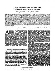
In this section, we briefly present some simulation results illustrating the performance of the index policy and the quality of the upper bound. We generate sites with random rewards R' within given bounds and random parameters P11, P2 1. We progressively increase the size of the problem by adding new sites and UAVs to the existing ones. We keep the ratio M/N constant, in this case M/N = 1/20. When generating new sites, we only ensure that Pu - P2 1 is sufficiently far from 0, which is the case where the index policy departs significantly from the simple greedy policy. The upper bound is computed for each value of N using the subgradient optimization algorithm. The expected performance of the index policy and the greedy policy are estimated via Monte-Carlo simulations. Fig. 4-8 shows the result of simulations for up to N = 3000 sites. We plot the reward per agent, dividing the total reward by M, for readability. We can see the consistently stronger performance of the index policy with respect to the simple greedy policy, and in fact its asymptotic quasi-optimality.
4.6
Conclusion
We have proposed the application of Whittle's work on restless bandits in the context of a mobile sensor routing problem with partial information. For given problem parameters, we can compute an upper bound on the achievable performance, and experimental results show that the performance of Whittle's index policy is often very close to the upper bound. This is in agreement with existing work on restless bandit problems for different applications. Some directions for future work include
a better understanding the asymptotic performance of the index policy and the computation of the indices for more general state spaces.
Chapter 5
Scheduling Kalman Filters In the previous chapter, we modeled the UAV routing problem as a sequential detection problem by assuming that the sites to be observed were independent two-state Markov chains. Suppose now that the sites or targets can be modeled as independent Gaussian linear time invariant systems, and that we would like to use the mobile sensors to keep a good steady-state estimate of the states of the targets. Similarly to the previous chapter, observations can only be made by the sensors if they travel to the location of the target. This is a variation of a problem considered by Meier et al., and Athans [91, 8]. In this chapter we apply the tools and ideas developed for the RBP to this estimation problem. The RBP provides the insight to derive a tractable relaxation of the problem, which provides a bound on the achievable performance. We show how to compute this bound by solving a convex program involving linear matrix inequalities. Exploiting the additional structure of the sites evolving independently, we can decompose this program into coupled smaller dimensional problems. We give the expression of the Whittle indices in the scalar case with identical sensors. In the general case, we develop open-loop switching policies whose performance matches the lower bound arbitrarily closely as the times for the sensors to switch targets tend to zero.
5.1
Introduction
We still have M mobile sensors tracking the state of N sites or targets. We consider here a continuoustime version of the problem. Let us now assume that the sites can be described by N plants with independent linear time invariant dynamics, i = Aixi +Biui+wi,
xi(O) =xi,o.
We assume that the plant controls ui(t) are deterministic and known for t > 0. Each driving noise wi (t) is a stationary white Gaussian noise process with zero mean and known power spectral density matrix W: Cov(wi(t), wi(t')) = Wi 3(t - t').
The initial conditions are random variables with known mean _i,o and covariance matrices Ei,o. By independent systems we mean that the noise processes of the different plants are independent, as well as the initial conditions xi,o. Moreover the initial conditions are assumed independent of the noise processes. We shall assume that Assumption 5.1.1. The matrices Ei,O are positive definite for all i E { 1,..., N}.
This can be achieved by adding an arbitrarily small perturbation to a potentially non invertible
matrix Ei,o. This assumption is needed in our discussion to be able to use the information filter later on and to use a technical theorem on the convergence of the solutions of a periodic Riccati equation in section 5.4.3. We assume that we have at our disposal M sensors to observe the N plants. If sensor j is used to observe plant i, we obtain measurements Yij = Cij x i + Vij.
Here vij is a stationary white Gaussian noise process with power spectral density matrix Vij, assumed positive definite. Also, vij is independent of the other measurement noises, process noises, and initial states. Finally, to guarantee convergence of the filters later on, we assume throughout that Assumption 5.1.2. For all i E { 1, ... , N}, there exists a set of indices jl, j such that the pair (Ai, i) is detectable, where .i = [CT1 ,. CT ]T.
Assumption 5.1.3. The pairs (Ai, Wi
/ 2)
...
Ji E
{1,...
,M}
are controllable,for all i E { 1,..., N}.
Remark 5.1.4. It is conjectured that in the following the assumption 5.1.3 can be replaced by the following weaker assumption: the pairs (Ai, Wi / 2) are stabilizable, for all i E { 1,... ,N}. Let us define 1 if plant i is observed at time t by sensor j
0 otherwise. We assume that each sensor can observe at most one system at each period, hence we have the constraint N
Erij(t)
1,
Vt, j=
1,...,M.
(5.1)
i=1
If instead sensor j is required to be always operated, constraint (5.1) should simply be changed to N 7ij ( t ) = 1.
(5.2)
i=1
The equality constraint is useful in scenarios involving UAVs, where it might not be possible to withdraw a vehicle from operation during the mission. The performance will of course be worse in general than with an inequality once we introduce operation costs. We also add the following constraint, similar to the one used by Athans [8]. We suppose that each system can be observed by at most one sensor at each time, so we have M
j(t) < 1, Vt, i = 1,...,N.
(5.3)
j=1
Similarly if system i must always be observed by some sensor, constraint (5.3) can be changed to an equality constraint M
E 7i(t) = 1.
(5.4)
j=1
We consider infinite-horizon problems, mostly in the average cost version and briefly in the discounted cost version. The parameters of the models are assumed known. We wish to design an
observation policy 7r(t) = {fij(t)} satisfying the constraints (5.1), (5.3), and an estimator 2, of x, depending at each instant only on the past and current observations produced by the observation policy, such that the average (or total discounted) error variance is minimized, in addition to some observation costs. The policy 7ritself can also only depend on the past and current observations. More precisely, we wish to minimize, subject to the constraints (5.1), (5.3), 1 Javg =
minlimsup-E T-oo
TN( Sx i=1
(x
-
,i)'Ti
-i,i) -+
(t) CEKiiji
j=1
dt ,
(5.5)
for the average cost problem, or Jp (o) = minE
e- t
(xi -
,i)'T(xi - X,i) + ~~ ij
i=1
(ij(t)
dt
(5.6)
j=1
in the discounted cost version. Here the constants iij are a cost paid per unit of time when plant i is observed by sensor j. The Ti's are positive semidefinite weighting matrices.
5.1.1
Modeling different resource constraints
A note on the generality of constraints (5.1), (5.2), (5.3) and (5.4) is useful. Allowing more measurements per system can be done without change in our discussion. Indeed, suppose (5.3) is replaced by M
E "ij(t) < Ki, j=1
for some i E {1,... ,N} and some constant Ki E {1,... ,M}. Then we create Ki copies of system i
and impose constraint (5.3) for each of them. In each of the copies however, we replace the matrices Vij by Vij/Ki. Then we sum the resulting Ki Riccati differential equations involving Ei. For example, if two sensors jl and j2 observe two copies of system i at the same time, this transformation is in effect equivalent to receiving the measurement Cijl
Cij2 1
vij,
0
0
ij2
for system i. Similarly, we could allow a sensor to observe several systems simultaneously if we allowed, quite unrealistically, that noise measurements remained independent for the two systems. Using (5.4) we can also impose a constraint on the total number of allowed observations at each time. Indeed, consider a constraint of the form NM
_,ri(t) < p,
for some positive integer p.
i=1 j=1
This constraint means that M - p sensors are required to be idle at each time. So we can create M - p "dummy" systems (we should choose simple systems, although satisfying assumptions 5.1.2 and 5.1.3, to minimize computations), and associate the constraint (5.4) to each of them. Then we simply do not include the covariance matrix of these systems in the objective function described above. In conclusion, it is sufficient for the modeling of a large number of problems to consider only constraints (5.1)-(5.4). Replacing the inequality by equality signs only changes trivially our discus-
sion. Finally, considering coupled measurement noise processes is also possible at the expense of increasing complexity in the computations of the assignment policies.
5.1.2
Literature Review
The sensor scheduling problem presented above, except for minor variations, is an infinite horizon version of the problem considered by Athans in [8]. See also Meier et al. [91] for the discretetime version. Athans considered only one plant to observe. We include here several plants to show how their independent evolution property can be leveraged in the computations, which is similar to the previous idea demonstrated for bandit problems (called dual decomposition method in optimization). Discrete-time versions of this sensor selection problem have received a significant amount of attention, see e.g. [43, 99, 126, 125, 54, 111, 117]. All algorithms proposed so far, except for the greedy policy of [111] in the completely symmetric case, either run in exponential time or consist of heuristics with no performance guarantee. However, to the author's knowledge, the problem has not been shown to be intractable. We do not consider the discrete-time problem in this thesis. Finite-horizon continuous-time versions of the problem, besides the presentation of Athans [8], have also been the subject of several papers [119, 107, 10, 83]. For these problems the solutions proposed, usually based on optimal control techniques, also involve computational procedures that scale poorly with the dimension of the problem. Somewhat surprisingly however, and with the exception of [94], it seems that the infinitehorizon continuous time version of the Kalman filter scheduling problem has not been considered previously. Mourikis and Roumeliotis [94] consider initially also a discrete time version of the problem for a particular robotic application. However, their discrete model originates from the sampling at high rate of a continuous time system. To cope with the difficulty of determining a sensor schedule, they assume instead a model where each sensor can independently process each of the available measurements at a constant frequency, and seek the optimal measurement frequencies. In fact, they obtain these frequencies by introducing heuristically a continuous time Riccati equation, and show that the frequencies can then be computed by solving a semidefinite program. In contrast, we consider the more standard schedule-based version of the problem in continuous time, which is a priori more constraining. We show that essentially the same convex program provides in fact a lower bound on the cost achievable by any measurement policy. In addition, we provide additional insight into the decomposition of the computations of this program, which can be useful in the framework of [94] as well. The rest of the chapter is organized as follows. Section 5.2 briefly recalls that for a fixed policy 7r(t), the optimal estimator is obtained by a type of Kalman-Bucy filter. In contrast to the previous chapter, the properties of the Kalman filter (independence of the error covariance matrix with respect to measurements) imply that the remaining problem of finding the optimal scheduling policy 7r is a deterministic control problem. In section 5.3 we treat a simplified scalar version of the problem with identical sensors as a restless bandit problem, and provide analytical expressions of the Whittle indices and of the elements necessary to compute the performance bound. Then for the multidimensional case, treated in full generality in section 5.4, we show that the lower bound on performance can be computed as a convex program involving linear matrix inequalities. This lower bound can be approached arbitrarily closely by periodically switching policies described in section 5.4.3.
5.2
Optimal Estimator
For a given observation policy
i(t)
= {ij(t)}i,j, the minimum variance filter is given by the
Kalman-Bucy filter [65], see [8]. The state estimates R, where subscripts indicate the dependency on the policy z, are all updated in parallel following the stochastic differential equation
IJ ij
(j=
dt ',i (0) = Xi,o.
The resulting estimator is unbiased and the error covariance matrix matrix Riccati differential equation dtai(t) = AiY,i(t) + E,i(t)Ai+Wi Ex,i()
-
Eri(t)
(
,,i(t) for site i verifies the
rij(t)CTVij'Ci)
YA,i(t),
(5.7)
= Ei,o
With this result, we can reformulate the optimization of the observation policy as a deterministic optimal control problem. Rewriting E((xi -. i)'Ti(xi -ii))
= Tr (Ti
i),
the problem is to minimize y= minlim sup -1 T--
Tr(Ti
(,i(t))+
i=1
o
L'Cij(t) dt ,
(5.8)
j=1
or
Jp (o) = min
e-Pt
i=1
Tr( iz,/(t))+ EKijfij(t) dt ,
(5.9)
j=1
subject to the constraints (5.1), (5.3), or their equality versions, and the dynamics (5.7).
5.3
Sites with One-Dimensional Dynamics and Identical Sensors
We assume in this section that 1. the sites or targets have one-dimensional dynamics, i.e., xi E R, i= 1,...,N. 2. all the sensors are identical, i.e. Cij = Ci, Vij = Vi , Cij =
li,
j = 1,...,M.
Because of condition 2, we can simplify the problem formulation introduced above so that it corresponds exactly to the type of bandit problems introduced in chapter 3. For this purpose, we define W
1 if plant i is observed at time t by a sensor 10 otherwise.
Note that a constraint (5.4) for some system i can be eliminated, by removing one available sensor, which is always measuring the system i. Constraints (5.2) and (5.3) can then be replaced by the
single constraint Ci(t) = M, Vt. i=1
This constraint means that at each period, exactly M of the N sites are observed. We treat this case in the following, as it is the standard formulation of restless bandit problems, but the equality sign can be changed to an inequality. To obtain the lower bound, we relax the constraint to lim sup1 f
i= 1
-T
T --
i(t)dt = M,
for the average cost problem, and
=l
e
i(t)dt = M
for the discounted cost problem. As explained in chapter 3, we adjoin this constraint using a (scalar) Lagrange multiplier A and we are led to consider for each site ()
= m 7tj
1
lim sup -T T-*oc
Tr(Ti Y,i(t)) + (ii + X) zi(t)dt,
Tfo
for the average cost problem. Here i is the cost per time unit for observing site i. For the discounted cost problem, we need to consider for each site J' (Ei,o,A) = minj e-
t
{Tr(Ti-r,i (t)) + (i+X)7ri (t)}dt.
The dynamics of E,,i are now given by d-
,i(t) = AiYr,i(t) + Yr,i(t)A + Wi - ri (t) c,i(t)CVi-l CiY,i(t),
(5.10)
EzC,i(0) = Yi,0o
If the dynamics of the sites are one dimensional, i.e., i E IR,we can solve this optimal control problem for each site analytically. That is, we obtain an analytical expression of the dual function which provides a lower bound on the cost for each A. Additionally, we can obtain an analytical expression for the Whittle indices. The expression of the Whittle's indices for first order deterministic systems was given by Whittle [136] and Dusonchet [39], assuming that the smooth-fit principle holds. In fact, their expression is not valid over the whole state-space and we correct this mistake in this section. We will also change the notation slightly for this one-dimensional problem and define qi := Wi,
ri := Vi.
We can consider the problem for a single site, dropping the index i. The dynamical evolution of the covariance obeys the equation C2
= 2aE+ q- 7-
E 2,
with 7r(t) E {0, 1}.
The HJB equation is y(A) =min E+(2aE+q)h'(E;,),E+K+ +(2aE+q -
E2)h'(E;£) ,
in the average cost case, and
Pv(E;I)= min E+(2ar+q)V(E;a),E++
+(2a+q-
E2)V(;)
in the discounted-cost case. We will use the following notation. Consider the algebraic Riccati equation 2 c
= 0.
2ax + q - -x r
Note that by the observability assumption 5.1.2, we have c > 0. Then, this equation has two roots x=
a22 + cq/r c /r
a-
x2
a+
2 2
+ c2 q/r r
is strictly positive, unless a = q = x2 = 0. xl is strictly negative, or 0 if a > 0 and q = 0. By assumption 5.1.3, the pair (a, q) is controllable. In fact, stabilizability is sufficient to imply a < 0 if q - 0 and so x 1 is strictly negative and x2 is strictly positive. x2
5.3.1
Average-Cost Criterion
We perform the calculations for the average cost criterion, which leads to simpler formulas. A similar treatment is possible for the discounted cost criterion. First, we can treat the case i + 0 immediately. Then it is obviously optimal to always observe, and we get, letting E = x2 in the HJB equation: y() So from now on we can assume
)
= X2
IC+.
> - KI.Note that here X has the interpretation of a tax for activity
instead of a subsidy for passivity as in chapter 3. Now let us temporarily assume the following result on the form of the optimal policy. Its validity can be verified a posteriori from the formulas obtained below, using the fact that the dynamic programming equation provides a sufficient condition for optimality of a solution. Conjecture 5.3.1. The optimal policy is a threshold policy, i.e., it observes the system for E > T and does not observe for E < T, for some T E R+. Now we would like to obtain the value of the average-cost y(X) and of the threshold T (X) or its inverse A(T). Note that we already know T(X) = 0 for 2 < -K. Inverting the relation H-T(2) gives the Whittle index, assuming that T (a) is an increasing function of X. Case T _ X2 In this case, we obtain as before y(X) =x2 + K 2+ .
(5.11)
This is intuitively clear for T < x2: even when observing the system all the time, the variance still converges in finite time to a neighborhood of x2. Since this neighborhood is in the active region
by hypothesis, after potentially a transition period (if the variance started at a value smaller than T), we should observe always, and hence the average cost is the same as for the policy that always observes. By continuity at the interface between the active and passive regions, we have T + (2aT + q)h'(T) = T + (i + X) + (2aT +q- -T2)h'(T) r 2 c
K+c =
r
T2h'(T).
We have then 2
-T
r
(x 2 ±
= -T 3 + (2aT +q)(Kc+
2)
r
(-T +aT+q
) C22 (+)=-T2(X2 - T)
c2
r
-(T-x T so
2 -
r
2
2 )(T-Xl)(
+)L =T (x 2 -T)
T(K+X) +xi(K+) T2 T- xi
= -+
)
(assuming c
0)
= 0
T()
=
K+
-
( +)(+A-2,
2(T) 2
- 4x)
(5.12)
Expression (5.13) and (5.12) are valid under the condition
T(2) =
+
X2.
Note from (5.12) that T - X (T) is indeed an increasing function.
Case T > x 2 It turns out that in this case we must distinguish between stable and unstable systems. For a stable system (a < 0), the equation 2ax + q = 0 has a strictly positive solution Xe = -
> x2.
Stable System (a < 0)with T > xe: In this case we know that we get
Xe
is in the passive region. Hence, with E =
r(X) =xe. Then we have again 2
K+X= C-T 2 h'(T),
r
and now T + (2aT +q)h'(T) = xe.
Xe
in the HJB equation,
(5.13)
Hence -T2(
r
e- T) = (2aT +q)(+
1(T) = -Kf+
c 2T 2 c 2+aYr
T()
) = 2a(T-xe)(K+ =
)
2|a r(, + K) c
(5.14)
|c|
Stable System (a < 0)with x2 < T < Xe, or non-stable system (a > 0): If the system is marginally stable or unstable, we cannot define xe. We can think of this case as Xe -+ oo as a -- 0_, and treat it simultaneously with the case where the system is stable and x2 < T < Xe. Then x2 is in the passive region, and Xe is in the active region, so the prefactors of h'(x) in the HJB equation do not vanish. There is no immediate relation providing the value of y(),). We
will use the smooth-fit principle to handle this case and obtain the expression of the Whittle indices, following [136]. Note that this approach alone is insufficient as it misses the cases treated above. Theorem 5.3.1 ([136],[39]). Considera continuous time one-dimensionalproject x(t) E R satisfying x(t) = ak(x), k= 0,1, with passive and active cost rates rk (x), k = 0,1. Assume that ao (x) does not vanish in the optimal passive region, and al (x) does not vanish in the optimal active region. Then the Whittle index is given by [al (x)- ao(x)] [ao(x)(rl)'(x) - al (x)(ro)'(x)] ,(x) = ro(x) - r1(x) + ao(x)[(a)'(x) - - a(x)[(ao)'(x) -3] in the discounted case, and h(x) = ro(x) - rI(x) +
[al(x) - ao (x)][ao(x) (rl)'(x) - al (x)(ro)'(x)] ao(x)(al)'(x) -al(x)(ao)'(x)
in the average-cost case. Remark 5.3.2. The assumption that ao and al do not vanish, capturing the cases previously studied, is missing from [136],[39]. Proof We give for completeness some details skipped in the proofs of [136], [39, p.53], which use the smooth-fit principle. A more rigorous proof should be possible, using variational inequalities. The HJB equation for the discounted-cost case is 3V(x) = min{ro(x) +aoV'(x), rl (x)+
+ alV'(x)}.
Hence, under our non vanishing assumption for ao and al 3_V-ro V'(x) =
ao 3v-r-1 al -
in the passive region (5.15)
in the active region.
Continuity of V on the boundary gives aoV' + ro = al V' + rl + 1
on the active-passive boundary.
Looking at the continuity of the second derivative of the value function on the boundary (as-
suming the smooth-fit principle to be valid), we obtain the additional relation: ao(
V' - ro) - a'o(PV - ro)
al(PV'-
PV' - ro - aoV ' pV' a a0 V'(a1 (p - aO) - ao(P - a)) = a!ro -
r') - a' (PV - ri - 1)
r1 - al V/ ausing
on the active-passive boundary
(5.15)
al
aor' .
Hence we obtain, = ro+-rl r +
(ao - al) (air - aor')
al ( - a') - ao(p - al)
The average-cost result is obtained for / = 0 or directly by the same type of argument.
Corollary 5.3.3. The Whittle index for the case x2 < T < Xe is given by: T3
c2
(T) = -~K+
(5.16)
2r (a+ P/2)T+q
in the discountedcost case, and
c2 T 3 2r aT + q
X(T) =-+
(5.17)
in the average cost case. Proof We have a0 (E ) = 2a E + q,
a l ( E ) = 2aE +
,
C E+ K r (E)=
q
c22 r
ro(E) =
We get in theorem 5.3.1 _C2y
S(E=
--
r
(2a + q) (2a - 2 4
Y
C 3~=
-K-
;1 (z) =K
r2 C2
£2
r 2E2)
(2a -/)
4
r2 -(2a£ + q)2 L+ 4
2
C
-/ ) - (2a + q E
C
(-)=K-
2
L2(2a
-/)
3
2a r - 2-q r
-
r
c2
Y3
2r (a + p/2)E + q The average-cost expression is obtained by formally setting P = 0. With the value of the Whittle index, we can finish the computation of the lower bound y()L) for the case x2 < T < Xe. Our task of solving the HJB equation has been simplified by the use of the smooth-fit principle leading to the expression of the Whittle indices. Inverting the relation (5.17),
A ()
- 1C
Figure 5-1: Whittle index for one-dimensional dynamics. we obtain, for a given value of X, the boundary T () between the passive and active regions. T(A) verifies the depressed cubic equation X3
2r
3
-( + K)aX -
22r
(A + )q = 0.
(5.18)
For A + K > 0, by Descartes' rule of signs, this polynomial has exactly one positive root, which is T(X). The HJB equation then reduces to y(A) =x+h'(x)(2ax+q), forx < T(A)
r(A) = x+
K+
+h'(x)(2ax + q -
r
x2),
(5.19) forx > T((),
(5.20)
with h, h' and h" assumed continuous on the boundary between the active and passive regions. Now for x2 < T(k) < Xe, with x = T(A) > 0 in the HJB equation, eliminating h'(T(A);X), we get
(y(X) - T(X)) y()
= T() +
c2
C2
1C
)=+(-Tr )+
(T(I))
2
2aT()+q q
(T(X)+q
=
+
r( c + )(2aT(A) + q) c2 (T()) 2 ,
forX2 - Oi(T)WiQi(T), and so we obtain ,,
1i11 I(Qi(T) - Qi,o) -< -Oi(T)Ai -AT Q(T) r
T
-A
Oi()
i(T)Wii(T) + -!j(T)j!OjT)T
i(
)C/TVi
1
Cij.
(5.27)
Last, since Qi(T) >- 0, this implies, for all T, M
ai(T)AT+ATi(T)+ Oi(T)Wii(T) - E ifij(T)CVijv'Cij j=1
SQi,o
T
(5.28)
So we see that for a fixed policy z and any time T, the quantity
Tr(Tii(T)) +
i 1j
1
(T)
(5.29)
is lower bounded by the quantity N
Tr(Ti (Q)i(T))-I) +
cijRiij(T)
i= 1
,
where the matrices Oi(T) and the number fij(T) are subject to the constraints (5.28) as well as N
M
fij(T)= 1, j =1,...,M, E itij(T) < 1, i= 1,...,N.
0 < ftj(T)< 1, i=1
j=1
Hence for any T, the quantity Z*(T) defined below is a lower bound on the value of (5.29) for any choice of policy r7 N{ Z*(T) = min
Tr(T
EiP,
+
i=1
Qi,Pij
(5.30)
j=1 M
s.t. QiAi +AT Q
T.
Q iWii--
PijCijVi
- 1i,o
Cij
-T'
, i= 1...,N,
(5.31)
j=1
Pij
1, j= 1,...,M,
i=1 M
Pij < 1, i= 1,...,N. j=1
Consider now the following program, where the right-hand side of (5.31) has been replaced by
{
N
Z* = min
M
r(Ti~
ii,Pij
i=I
pijPiJ
(5.32)
j=1 M
s.t. (QiAi+Ai
i
OiWiii
N pij < 1,
j=
1,...,M,
i=1 M
SPij j=1
1, i = 1,... ,N.
-
PijCijVi 'Cij -4 0, i = 1...,N,
(5.33)
Defining 6 := 1/T, and rewriting by slight abuse of notation Z*(6) instead of Z*(T) for 6 positive, we also define Z*(0) = Z*, where Z* is given by (5.32). Note that Z*(0) is finite, since we can find a feasible solution as follows. For each i, we choose a set of indices Ji = {jl,..., ni} C { 1, ... ., M} such that (Ai,Ci) is observable, as in assumption 5.1.2. Once a set Ji has been chosen for each i, we form the matrix P with elements Pij = 1{j E Ji}. Finally, we form a matrix P with elements Pij satisfying the constraints and nonzero where the Pij are nonzero. Such a matrix P exists as a consequence of Birkhoff theorem, see theorem 5.4.2. Now we consider the quadratic inequality (5.33) for some value of i. From the detectability assumption 5.1.2 and the choice of Pij, we deduce that the pair (Ai, i), with Ci
V1/2
=
"'
Vii
is detectable. Also note that
-1/2 i(5.34)
---
PiMCiM vim
(5.34)
M
Tci =
PijCjVi
Cij.
j=1
Together with the controllability assumption 5.1.3, we then know that (5.33) has a positive definite solution Qi [1, theorem 2.4.25]. Hence Z*(0) is finite.
We can also define Z*(6) for 6 < 0,by changing the right-hand side of (5.31) into 6Qi,o - 1Qi,o. We have that Z*(6) is finite for 6 < 0 small enough. Indeed, passing the term 6Qi,o on the left hand side, this can then be seen as a perturbation of the matrix Ci above, and for 6 small enough, detectability, which is an open condition, is preserved.
We will see below that (5.30), (5.32) can be recast as convex programs. It is then a standard result of perturbation analysis (see e.g. [23, p. 250]) that Z*(6)is a convex function of 6, hence continuous on the interior of its domain, in particular continuous at 6 = 0. So limsupZ*(T) = lim Z*(T) = Z*. T-+
T--+oo
Finally, for any policy 7, we obtain the following lower bound on the achievable cost 1
limsup T--.,
To
N
Tr(TiYi(t))+
i=1
M
i1Ciij(t) dt > lim Z*(T) =Z*
j=1
T--+
We now show how to compute Z* by solving a convex program involving linear matrix inequalities. For each i, introduce a new (slack) matrix variable Ri. Since Qi >-0, Ri >- Q- 1 is equivalent, by taking the Schur complement, to Ri
I
I
Qi
>0
and the Riccati inequality (5.33) can be rewritten Oa+
-
i
Wi
1 2
/
=lC1ij
/ijC i
I
Ci
I-I
- Ef(t) is the positive definite periodic solution of the PRE (5.40). It is eperiodic. From Radon's lemma [1, p.90], which gives a representation of the solution to a Riccati differential equation as the ratio of solutions to a linear ODE, we also know that Ef is C' on each interval where ai(t) is constant, where oi(t) is the switching signal defined in the proof of lemma 5.4.3. Let
i
be the average of t-
F (t): 1
S= e,(t)dt.
From the preceding remarks, it is easy to deduce that for all t, we have if (t) integrating the PRE (5.40) over the interval [0, E], we obtain
Jo
^fA
Now, 0 = O(e).
S11
(t)(t)dt=
(t)(c (t)
- F(O))=0.
Expanding this equation in powers of e, we get Aif +A .f
(CI(t))c(t)dt
+Wi-i -,
+ k-I )E, (l+ 01 +... + k)e]. We can then
where R(e) = O(e). Let jk := Ci(t) for t E [(I + 01 rewrite e c 1 fo dt -e (Cf(t)) Cf(t)
+R(e) =0,
OTcc7 'CK Cijk. ykCjaijk #
V '
k= l
Let us denote by Pk,ij the (i, j)th element of the matrix Pk in (5.39). We have Pk,ij - l{j=jk with the
above definition of jk, including the case jk = 0 (no measurement), which leads to Pk,ij = 0 for all j {1,... ,N}.Then we can write k k-=1
N
K
K
kVi
C
kijC V
Ok k=1
j=1
S OkPk,ij
k=1
N j= 1
PijCijVij
Cij
M j= P1ijCVU1
j=1
i
j=1
CV C
(5.43)
where the last equality uses our convention Vi-
1
0 for j > M + 1, and the fact that Pij = Pij for
=
j < M. So finally, we obtain
(
Aie + ieA T + (Wi +-R(E)) -
pijC ViC-1i)
Note moreover that Ef is the unique positive definite stabilizing solution of this ARE. Now comparing this ARE to the ARE (5.42), and since the stabilizing solution of an ARE is a real analytic function of the parameters [35], we deduce that
- E = O(e), and the lemma.
Theorem 5.4.5. Let ZE denote the performance of the periodicswitching policy with period e. Then Z e - Z* = O(E) as E - O, where Z* is the performance bound (5.35). Hence the switching policies
approachthe lower bound arbitrarilyclosely as the period tends to 0.
Proof We have ZE = limsup
T
T- oo
rr(Ti (t)) + i=1
Kj f (t)
dt,
j=1
where 7'E is the sensor/system assignment of the switching policy. First by using a transformation similar to (5.43) and using the convention ij = 0 for j E {0} U {M + 1,..., N} (no measurement or
measurement by a dummy sensor), we have for system i
I T
M
1 i-
3E j=1
T n=
(n+1)e
1
T
Ji
7
T
KI1 )+ Tj S Ek=1ETJ
LTJ j p
+
1 su
N
T-+o
1
T
iT
Eijj
yjJ j=l
T] j 1 N
M
lim sup T
j=
i (t)d t
- T M ij7rij (t)dt.
T E Hence
T
M
ij7j(t)dt < i=1 j=1
(5.44)
KijPij. p i=1 j=1
Next, from lemma 5.4.3 and 5.4.4, it follows readily that lim supt, E'(t) - E* = O(E). It is well known [127] that E* is the minimal (for the partial order on S') positive definite solution of the quadratic matrix inequality Aii +
A +Wi - Ei
PijCVi
(j= 1
Cij
Ei -
rai -
i=1 .a i
(Xai) - Csia 1i
M
}
i=1
which is the inequality obtained by using the vector (6.19) in the constraints of (6.5). The case where si = ai for some i is almost identical, considering the constraints (6.18) for the O corresponding indices. In the following theorem, using the notation of section 3.2.3 we will use the occupation measure (state frequency) Fa (v, i~)on the state space, which we define from the state-action frequency simply as
fa (v,
Fa (v, ii;x,s) =
i; x,s,a), V(x,s).
aErl[N]
Let g to be the Theorem 6.6.2. Let v be an initialdistributionon the states, of the productform (6accordin). optimal rewardfunction, J be an approximationof this rewardfunctionformed according to (6.19), and i~be the associatedone-step lookaheadpolicy. Let Fa (v, 17) and Ja be the occupation measure vector and the expected rewardassociatedto the policy ii. Then 1 vT(J*- J) < -lFa(v, )T( - J*), 1-a
(6.29)
or in other words, 1
1 Fa (v, 7; x, s) (J(x,s) - J* (x, s)). Ev(x, s) |J*(x, s) - Ja (x, s) I < x's I - a x's
In words, the theorem says that starting with a distribution v over the states, the difference in expected rewards between the optimal policy and the one-step lookahead policy is bounded by a weighted ll-distance between the estimate f used in the design of the policy and the optimal value function J*. The weights are given by the occupation measure of the one-step lookahead policy. This result is true for every one-step lookahead policy that uses a superharmonic vector as an approximation of the cost-to-go. It gives some motivation to obtain a good approximation J and a tight relaxation. Proof We follow the analysis presented in [34]. First, by lemma 6.6.1, the vector J in (6.19) is a 119
feasible vector for the linear program (6.5), and since J* is the optimal solution we have vT > VTJ*.
(6.30)
For an action a E 1[U], we denote by ga the vector of immediate rewards, i.e., from the definition (6.21), ga(x; s) = g((x; s), a). Recall also the definition (6.22) of the transition matrix Jxax'. Let Ta and T the dynamic programming operators (TaJ)(x;s) = ga(x;s) +a
1
JSxaxJ(x';a),
X'Ey
(TJ)(x;s) = max
ga(x;s)+a xJ
xax,J(X';a)).
For a deterministic stationary policy u : Y x I[N] -- HI[N], we will also simply write u instead of u(x, s) when it appears as a subscript. Then the cost Ja of policy 1 defined in the theorem is the solution of the linear system J - TaJa. If we also denote by Pa the stochastic matrix Oxa(x;s)x,, this can be written as
Ja = ga + aPJJ. Now (I - aP) has an inverse since Pa is a stochastic matrix and a < 1, so we get Ja = (I - aPa)- ga. Moreover, under policy ii, the state of the system evolves as a Markov chain, and we have Iuv(X = x, St = ) = [TPatxs. So the occupation measure is Fa(v,5) = (1 - a)
atvT
= (1 - a)vT(I-
Pa)-
.
(6.31)
t=O
Now f-Ja
= (I-
aPa)-
[(I- aP,)f- ga] = (I-aP,7)-
1
[f- (ga + aPJ)] .
By the definition of the one-step lookahead policy ga + aPJf= Ti. So we obtain
f- Ja = (I - aP)- [i- TJ . Then starting from (6.30) and using (6.31) vT (J* -Ja) < VT(f
Ja)
Ti. Then by the monotonicity of the operator T the fact that limN,.
TNfj= J*, we obtain TfJ> T 2J > ... > J*. So
T (J* _- J
)
0, C(x) < 1, where C(x) is called the constituency matrix when the server is at position x. The dynamics of the queues are described by the following differential equation dqi(t) =
- i(x(t))(t)
dt
(
,
(7.2)
qi
where d denotes the right derivative, and we use the notation (g(x))
g(x) if y > 0 max(g(x),0} if y = 0.
We can also add constraints imposing finite buffer sizes. Fig. 7-2 shows an example of a filling rate profile for a one-dimensional problem with service rate ki(x) linearly decreasing with the distance xli to the queue. The vector field in (7.2) enforces the nonnegativity constraint for the fluid levels in the buffers, and is discontinuous on the boundary where qi = 0 and a - i(x) i< 0. Example 7.2.1. Two stations transmit a signal to the mobile server (UAV) over a shared additive white Gaussian noise channel, with power Pi, i = 1,2. The server, when at position x, receives the signal from station i with power pi(x) = Pi/(Ci + lIx - xi )ai, where Ci and ai are constants, and 125
x i is the position of the i t h base station. If the server decodes the transmission of the base stations sequentially, it can achieve communication rates Ri(x) that are subject to the following constraints [33]: Ri < log(l + pi(x)), i= 1,2, and Ri +R2 < log(l+ pl(x) + p2 (x)). To put this example in our framework, we can let Li(x) = log(1 + pi(x)) for i = 1,2, Ri = pi(x) i
and rewrite the constraints 0
0, C(x) < }.
In addition, there are additional implicit constraints on " when q hits the boundaries of Q, to prevent the queue lengths from violating their positivity or finite buffer size constraints. In complicated networks, the matrix B might not be square and the components of correspond to different activities [92, chapter 6]. In the simple scheduling scenario described here however, B(x) is a diagonal matrix for all x, with Bii(x) = -i (x). The stability condition presented in section 7.3 is valid for the general model (7.3) however. Finally, note that models of the vehicle dynamics much more general than (7.1) could be used. In fact, the dynamics of the vehicle do not play a role to obtain our stability condition for the fluid model, except for the fact that (7.1) allows the control law to stop the vehicle at an arbitrary location of the state space X. Hence the stability condition presented below is valid for any vehicle that can stop at any x E X (for example, a double integrator, or a Reeds-Shepp vehicle) but would have to be adapted to work for the Dubins vehicle for example. '
7.3
Stability of the Fluid Model
In general, it is not possible to drain all queues to zero simultaneously using the mobile server, if the intersection of the draining regions, which are the regions of X where the server can drive the queue level of a particular queue towards 0, is empty. Hence we use the following weaker notion of stability. Definition 7.3.1. The system q is said to be stabilizable if there exists constants K and T such that, for any initial condition qo, Jq(t)[II < K Vt > Tqo0oll-. 126
Remark 7.3.2. The requirement to bring the queue sizes close to 0 in a time proportional to IIqo01 is without loss of generality, as should be clear from the dynamics (7.3) and the geometric picture presented in the following.
To study the possible trajectories of the vector q in (7.3), we will study the velocity space for the queues, generalizing the corresponding definitions in [92]. Let Y= U{{x}xU(x)}. xEX
First we note that a trajectory (x(t), 4(t)) defines for each T E R+ a probability measure Px', on Y where Pr' (A) is the proportion of time that the pair (x, 4) spends in set A C Y in the interval [0, T]. In other words PT'1(A)=
Sx(rt),(t)(A)dt.
Then, integrating (7.3), we obtain, for all T E R+, q(T)= qo+a+rT+
B(x(t))4(t)dt
q(T) = qo + aT + T q(T) = qo+ aT + T
B(x)'Sx(t), (t)(dx,d4)dt B(x) P P (dx,d4).
(7.4)
Define the velocity space for the queues as V = {+
IB(x) P(dx, d4) : P a probability measure on Y
.
Clearly, V is a convex set in RN . It is the set of directions in which we can steer the vector q, by moving the server and controlling the allocation rates 4, if we do not take into account the dynamical constraint (7.1) imposed on the vehicle dynamics. In fact, we will see below that this constraint does not play a role as far as stability is concerned. Now the following is useful for approximating the set V. Note that by definition of the Lebesgue integral, we can approximate
a +JB(x) dP(x,(), arbitrarily closely by the "Lebesgue sums" a
+
B(xk) kpk,
(7.5)
k=1
whereE pk - 1 (since P(Y) = 1), and xk E X, and ' k E U(xk), i= 1,... ,n. Such a sum correspond to a point in V with associated measure E,1 pk xk, 4 k. Let V(x) = {a +B(x)
:
E U(x)}.
For each position x of the server, V(x) is a convex polyhedron. Note that since 0 E U(x) for all x, all 127
these polyhedrons contain the point a. Then we define
UV(x) .
V = cony
Clearly V is the set of points of the form (7.5), and so V is dense in V. Note that since V and V are convex, this implies int(V) = int(V). (7.6) Let C E be the l" e-ball C
e -
= {v E IN: -E
0. Figure 7-3 shows the velocity set for an instance of the problem where a = 1,
a 2 = 3,
Pl(x) =
3
1XI
,
2(x)
4
1I+ x-4
(7.9)
(
Let us define the draining region of queue i as D' := {x
E R
ij
y i(x )
0, Vj, n. Hence by convexity the points - 1e {(,..., also belong to V. Finally recalling that a E V (with a E RN ) and again by convexity of V, we obtain that CE C V for e = 1/T. 2 = 3. Suppose CE C V, for some e. If CE \ {0} C int(V), then CE C V using (7.6), a E V and the convexity of V (we use this condition since it allows the case a = 0 on the boundary of V). The rest of the argument concerns the technical point which arises when facets of Ce are on the boundary of V. We prove that in this case, these facets are also in V. So assume that there is a point vo E CE \ {0} which is on the boundary of V. We call 9 the set of probability measures on Y. We also define, for P E -?, P(dx,d4).
v(P) = a+ jB(x) Then let P0 E 90 be such that v(Po) = V0 .
Since V is convex, there is a supporting hyperplane H c RN of V passing through vo. By a transformation of coordinates, we can assume that H is the plane XN = 0, and that for all P E 0, we have the coordinate [v(P)]N < 0. Considering Dirac measures, we have that for all (x, ) E Y, (a +B(x) )N < 0. In particular, taking
0 implies that an - 0, and so
V(x, ) E Y, (B(x))N < 0.
(7.12)
Now we have vO =
(B(x)¢)N P 0 (dx, d4) = 0,
which, with (7.12), implies that, except possibly for a set of Y of P 0 measure 0, we have (B(x) )N = 0. Hence we can restrict the problem of approximating the integral defining vo by using points B(xk) k which are on the hyperplane H. Repeating the same argument for an intersection of hyperplanes if there is a lower dimensional facet of CE (such as an edge) on the boundary of V, we see that we can always restrict the approximation problem for points v of the facet by using points B(xk) k which are on that facet. Hence the facet also belongs to V (by convexity of V again). So Ce C V. 3
1. The idea is intuitively clear. For T large enough, - E belongs to V, so we can write n
0 = qo +aT +T
B(xk)
kpk.
k=1
Then a policy which moves the server successively through the points xk, k = 1,..., n, uses at these points the allocation rates k, and spends time pkT at point xk drives the system approximately to 0 if T is much greater than the time spent traveling between the points xk. Moreover, this policy is approximately time optimal, since it drives the vector of queues in the most direct way possible towards 0. Of course, this reasoning is valid only for the case where qo,i is large for all i, for which the positivity constraints and the travel times can indeed be neglected, but this is the only case of real interest as far as stability is concerned. The argument is complicated however by the fact that the choice of the configurations (xk, 4 k), which determines the total travel time and the impact of the positivity constraints, depends on the travel direction -qo/T and it becomes problematic to obtain an upper-bound K independent of qo on the steady-state sizes of the queues. Hence we will show stability by driving the queues toward 0 using a single direction (the diag131
onal), sacrificing time optimality in the process. Let qo = (qo,1, ... , qo,N) be the initial queue sizes.
We start by bringing the queue size vector close to the diagonal D := {q E RN: ql = q2 *...= qN, as follows. For each j E {1,... ,N}, there is a configuration (xi, iJ)E Y such that vi = B(xJ) i E and verifies and v > 0,iS 0 such that E
, so - q1 = aT2 + T2
T2
for some configurations (xk,
n
B(xk)kpk,
k=1
),k = 1,...,n. Then by adapting the usual the policy that puts the
server in the successive configurations (xk,
k),
k = 1,..., n, we can move the queue size vectors by
-ql + 6 + aT 3 . Here 5 is a nonnegative fixed quantity which takes into account the effect of the positivity constraints, and T3 is the sum of the switching times between configurations. So at the end of the second step, the vector q is at the point 8 + a(Ti + T3). The duration of the second phase if proportional to Ilq I|, which can be bounded by a constant multiple of IIqo|. So the total time is can be written Tiqo II + aTl. Using the ideas above, it is not hard to see that there are constants K and K 1, for which we can choose KI 2 |6 + a(T + T3)I1, such that if IIq(to) I< KY 1 for some t, we can insure Iq(t) 11.< K, Vt > to (we can use the velocity vectors vJ of (7.13) for this purpose). Hence we are done by choosing T = + T1 , in the case IIqo I o > K1 .
Time Optimal Trajectories We conclude this section with a brief and informal discussion of time-optimal trajectories, that is, trajectories which bring the queues in the bounded region of definition 7.3.1 in minimum time. Assume that we start with an initial condition qo which is far from the boundaries, see Fig. 7-4. Then time optimal trajectories correspond to driving the queues in the direction -qo. This direction belongs to the velocity set if the system is stabilizable. However, it is possible that one can steer the queues in this direction only be traveling between different points in the space X. As long as we remain far from the boundaries of the state space Q, we can drive the queues approximately in the direction -qo. Problems arise, and in particular we cannot necessarily neglect the traveling time any more, once we approach the boundaries. 132
qo + a
I I I II ! I I I !
0
I
-
I
s
I I I S I S
-
Cql 0
Figure 7-4: Initial condition qo, velocity set (the gray polygon), and example of trajectory for the queues.
7.4
Trajectory Optimization for a Draining Problem
If a system is stable in the sense of definition 7.3.1, then we can implement it using finite buffers. Moreover, the proof of theorem 7.3.3 showed how to bring the queue levels below the upper-bound K approximately in minimum time, as least when starting from a large initial condition. The precise dynamics of the vehicle had no influence on the stability condition, but only on the values of K and T. There are other types of objectives one might want to optimize. If we want to give priority to certain types of jobs at certain locations for example, minimizing a weighted sum of the queue levels might be appropriate. In this section, we touch upon this problem, for which the dynamics of the vehicle play a more important role. To illustrate the ideas, we consider a simple particular case of the two-queue configuration (7.7), (7.8). We study the problem of drainingoptimally the fluid present initially in the system, when no new arrival occurs (i.e., al = a2 = 0) and we incur a running linear cost clql(t) + c2q2(t), with Cl, c2 strictly positive constants. 7.4.1
Server with Unbounded Velocity
If the server were allowed to travel with infinite velocity, there would be a path-wise optimal solution. Indeed, suppose that additionally to the points x attaining the maximum service rates j, there is a point x* realizing the maximum x* E argmax{c 1 l(x) + c2 2 () }. x Then, since we have dt c(q(t)) = -Cl [i (x(t))]+ - C2 [k2(x(t))]q 2 133
we obtain immediately Theorem 7.4.1. For the drainingproblem with linear costfunction and a server with infinite velocity, the following rule is path-wise optimal, i.e., for given initialfluid levels, it minimizes c(t) for all t > 0:
1. as long as qi > 0 and q2 > 0, place the server at x* 2. ifql = 0, place the serverat x, otherwise if q2 = 0, place the server at x (until the totalfluid reaches 0). Now define the infinite-horizon cost J(qo;u(.)) =
j
c(q(t))dt =
clql(t) + c2q 2 (t)dt,
(7.14)
and the draining time T(qo;u(-)) = min{t :q(t) = 0}, where qo = [qlo, q 20]T is the initial fluid level in the queues. A policy minimizing J(qo; -) is called infinite-horizon optimal, and it is called time optimal if it drains the system in minimum time. We have then Corollary 7.4.1. For a server with infinite velocity, the policy of theorem 7.4.1, being path-wise optimal, is also infinite-horizonoptimal and time optimal. Remark 7.4.2. If the draining regions do not overlap, the policy of theorem 7.4.1 chooses the position x* associated to the maximum value of the indices cipi*, i = 1,2. Hence, we recover the well-known "c/rule" [92]. 7.4.2
Necessary Conditions for Optimality
We now consider the optimization of the infinite-horizon cost (7.14) for a server with the simple dynamics (7.1) and bounded velocity. Using the minimum principle, we can derive necessary conditions satisfied by optimal trajectories. For each subset S of { 1, 2}, define the Hamiltonian HS(q,x, u,p) = Eciqi - EPipi(X) + pOU, iES
(7.15)
iES
which is the Hamiltonian for the system where S represents the set of non-empty queues, and p = [P0, P1, P2] are the adjoint variables. In contrast to standard optimal control problems for fluid models, where the draining rate is assumed to be under direct control, we cannot enforce the positivity constraint on the fluid levels by a simple state dependent constraint on the control. We must take into account the discontinuity in the dynamics of the system when a queue level reaches zero. Suppose that both queues are non-empty, that the server is in the draining region D i of queue i, and that queue i becomes empty at some time ;i. Suppose that there is only one queue becoming empty at time ri. From the results in [26, sections 3.5 and 3.6], at the boundary qi - 0,we have the following relations pi(Ti-) = pi(
)
+ ri,
pj(H2-) = p j (r+),
H1 I'2 }(ri-) =H{J('}r+), 134
j i j:4i
(7.16)
(7.17)
where 7i is a (constant) Lagrange multiplier. Now using the continuity of the state variables q, x and of the Hamiltonian (7.17), we get pi(i-)Pi(x(i-)) = 0,
and since the server must be in the draining region D' (where 2i(x(vi-)) > 0) when queue i becomes empty this implies pi(z)
= 0.
Hence, the adjoint variable corresponding to queue i vanishes at the time when the queue becomes empty. The optimal control is of the bang-bang type u(t) = -sign(po(t))V.
When the queues in the set S are non-empty, the adjoint equations are, iES
Pi = -Ci,
po = EPid (x(t)), iES
where the derivative with respect to x can be taken to mean a subgradient in the case of nonsmooth rate functions. From the first set of equations and the preceding argument, we deduce pi(t)=ci(ri-t), i
{1,2},
Finally, since the dynamics and cost function are independent of time and this is a free terminal time problem, we know that the Hamiltonian is constant and equal to zero along optimal trajectories.
7.4.3
Draining Problem with Two Distant Sites and Linear Rate Functions
In this section, we consider an example where the server starts initially on the line segment between two base stations located at positions 0 and d. We assume for simplicity that the stations are sufficiently far from the initial position of the server, so that the queue at each base station would become empty before the server can reach it, if it were to always move towards that base station. The objective is to drain the queues while minimizing the infinite-horizon cost function (7.14). We assume that the draining region of each queue covers the whole segment [0, d], so that even a immobile server is draining the queue in finite time. We also assume here that the service rate decreases linearly with the distance to the base station, i.e., pi (x) = po - sl Ix| and 12(X) = 120 - S2 d - xJ, with sl and s2 positive constants. In particular, in the region [0, d] of interest, we have /21(X) =
10--sIX,
22(x) =-
20
-s
2 (d -x),
xE [0,d].
Calling the terminal time tf, we have tf = zl or tf = 2 and also H(tf) = -Vlpo(tf)l = 0
=
po(tf) = 0.
(7.18)
We determine the optimal trajectories by considering different cases based on which queue becomes empty first. 135
Case 2
z2 , we have, for x in the region [0, d], Po = -Pis] = ciSl (t- Z1).
This gives, with the condition (7.18), 2 (Zi - t)2 , fort E [r2 , rl].
Po =
Hence po is strictly positive on (r 2 ,zl) and and so during that phase, we have u = -V, i.e., the server moves towards the left base station, as expected. Now consider the time r2, at which we have po0( [0, T2 ), we have Po
= -P
+P2S2
2)
= -C1SI (1
> 0 and po is continuous. On the interval - t)
+
C2S 2(
2
- t).
This equation, together with the continuity condition at T2, gives C1S1
Po = If cIsl
= C2S 2 ,
2
C2S2
(r(zl-t)-
then po = clsl (li - ,2)
( +2
t) 2 , fort E [0,Z 2].
-2
2
t) and so po remains positive and the server must
-
always move towards the left base station. This is also true if c i sl > c2S2. Now in the case C2S2 > clsl, there is potentially a time to > 0 such that on [0, to), po(t) is negative and the server must move towards the right base station. We obtain to by solving for po(to) = 0, so that, defining _ R:= ~Is Sc2S2
we get to = max
(t
2 -
2-t 1 - to
1
1- Ri
,O
(7.19)
which is positive if and only if T2 > z 1R. In conclusion, for an optimal trajectory to empty queue 2 first, the server must necessarily be always moving to the left if R > 1, and if R < I it must be moving right for time to and then left. Consider the case R > I first. If the server always moves left, we have
x(t) = xo - Vt. This gives (assuming that the server does not reach station 1 before tf): l
(t) = -910
+ six(t) = -A10 + sixo - sl Vt, t2
q1 (t) = q1,o + (slxo - #10)t - sV2
4 2 (t) = -P20 + s2(d- x(t)) = -#20 + S 2 (d -xo) q2(t) = q2,0 + (S2 (d - xo) -
136
2 0)t
t + S2 V -
2
2
+ s 2 Vt
Letting qi (lI) = 0 and q2 ( 2 ) = 0, we get :1 := 71,l
72 " 72,1 =
(SIXO -- #10) + /(SixO
(7.20)
- y10)2 + 2siVql,o
(7.20)
siV -(s
2 (d -
xo) -
20) -
(S2 (d - xo) -20)2
- 2s2Vq2,0
s 2V
(7.21)
recalling that (sixo - P10) and (s 2 (d - xo) - 20) are negative quantities by assumption. The trajectory for the queue level q2 (t) is a convex function of t and the time 7r 2 corresponds to the smallest root of the equation q2(t) = 0. With these quantities and R > 1,for the optimal trajectory to empty queue 2 first, we must have r2,l < r1,,. This gives a condition that depends only on the parameters of the problems. If this condition is not verified and R > 1,then queue 2 cannot empty strictly before queue 1.
Now suppose R < 1. As long as 72 < RTl, the optimal solution must again move the server always to the left. So for such an extremal solution to exist, we must have v2,1 < RT,1. If we find that 2 ,1 > RT 1,1, always moving the server to the left cannot be optimal, but we might still have an optimal solution which empties queue 2 first by first moving to the right. Let ti(tr) be the time at which queue i empties if the server first moves right for a time t,,and then left. Thus, we are considering the case R < 1, Rl (0) < 72 (0). As we increase tr, r2 (tr) decreases and r (tr) increases. The positive time to verifies the equation (1-R)to = r 2(to)-Rl(to),
(7.22)
fort 0 > 0
(tr) and solving the fixed point equaso we have reduced the problem to computing the functions i; tion (7.22), i.e., finding the intersection of the diagonal with (r2 (tr) - Rt (tr))/(1 - R), a decreasing
function of tr. Once we have obtained to, we can verify if the optimal solution indeed empties queue 2 first by verifying 2(to) < i (to). If not, again, the optimal solution cannot empty queue 2 strictly before queue 1. Note also that when r2 approaches rlfrom below, i.e., both queues empty at the same time, we get to - 71 = tf, and so in the limit we should move the server to the right all the
time.
Now when the server moves to the right first for time tr, we have x = xo + Vt, and we get
2 ql(tr) =max 0,ql,o + (slxo
-
O)tr +siV-
(7.23)
,
q2(tr) = max 0, q2 ,0 + (s 2 (d - xo) - #20 )tr - S 2 V
.
(7.24)
Note that in fact, from the argument above, for 72 < T1, tr must be such that ql (tr) and q2 (tr) are both positive, since when queue 2 empties at r2, we must be traveling left and have passed the time tr. This constrains the set of possible values to consider for tr. Then we can replace qi,o by qi(tr) 137
and x 0 by xo + Vtr in (7.20), (7.21), to obtain l
(Si (xo + Vtr) - 10o)
= tr /(tr)
-
siV
(sl (xo - Vtr) - y10)2 + 2s V (qlo + (slxo -
tlO)tr
+
sg V
siV -(s2(d - xo - Vtr) - 920)
Z2(tr) = tr +
s2V
(s2(d - xo- Vtr) -
20)2 - 2s2 V (q2,0
+ (s2 (d-xo) - 120)tr- S2V)
s2 V
From these expression we can compute to by solving the fixed point equation. It reduces to finding tr such that (P20 - s 2 (d - xo - Vtr)) -
= (R
+
(\s2 (d-xo-Vtr)S2
S
;(Si (xo
(
(XO + Vtr) -
20) 2 -2s
2V
q2,0+s+ 2(d-xo) -
20)tr-s
2V 2
,10)
+ Vtr) - ,1O)2 + 2s1V (ql,o + (siXO - plo)tr-+Y sV
)
}.
In practice, the feedback solution, discussed later, is more useful than the open-loop control and does not require finding the value of to. However, to could be useful for computing performance bounds, or t design an open-loop policy if we don't have access to the updates on the sizes of the queues or the position of the server.
Case Z1 < 72 The analysis is identical to the previous case, interchanging the indices in the first part, and V with -V. Let us repeat the details for completeness. For t > rl, we have, for x in the region [0, d], Po = P2S2 = -C
2 S2
(t -
r2)-
This gives, with the condition (7.18), Po
CS2 (2 - t)2, for t E [72 ,Z].
Hence po isstrictly negative on (72, 1) and and so during that phase, we have u = +V, i.e., the
server moves towards the right base station, as expected. Now consider the time r1,at which we have po(7l) < 0 and po is continuous. On the interval 138
[0, zl), we have Po = -plsI + p2S2 -= _-CiS
1 - t) + C2S2(T2 - t).
This equation, together with the continuity condition at r2, gives again C1S1
Po = 2 ( 2
If c 1sl = c2S2, then po = cls l(z -
2
- t) 2 2)
C2S2
2 - t) 2 , fort E [0,
2
2
and so po remains negative and the server must
-t)
(~
2].
always move towards the right base station. This is also true if c1s] < c2S2. Now in the case clsl > c2S2, there is potentially a time to > 0 such that on [0, to), po(t) is positive and the server must move towards the left base station. We obtain to by solving for po(to) = 0, and defining like before lS _ T2-
R :=
t '1 - to
Sc2S2
we get to =
ax
R-2
(7.25)
which is positive if and only if 2 < zlR, since we now have R > 1. In conclusion, for an optimal trajectory to empty queue 1 first, the server must necessarily be always moving to the right if R < 1, and if R > 1 it must be moving left for time to and then right. Consider the case R < 1 first. If the server always moves right, we have x(t) = xo + Vt. This gives (assuming that the server does not reach station 2 before tf): 1(t) = -ilo
+ six(t) = -i
1o +
sixo + siVt, t2
q1 (t) = qi,o + (sixo -
0io)t + siV
42(t) = -P20 + S2(d - x(t)) = -920 + s 2 (d - xo) - s 2 Vt 2
q2(t) = q2,0 + (s 2 (d - xo) -
#20)t
t - s 2 V-.
2
Letting qi(ri) = 0 and q2( 2) = 0, we get T1 :=
=
= 2,r =
(#lo - sixo) -
/(sXo -
siV
1o) 2 - 2sVqo 2,r
(s 2 (d - xo) - #20) + V/(s 2 (d
s2
s2V
-
xo) - /20)2 + 2s2 Vq 2 ,
(7.26) (7.26)
(7.27)
recalling that (sixo - y1o) and (s 2 (d - xo) - y20) are negative quantities by assumption. The trajectory for the queue level qi (t) is a convex function of t and the time rz corresponds to the smallest root of the equation ql (t) = 0. With these quantities and R < 1, for the optimal trajectory to empty
queue 1 first, we must have zl,r < Z2,r. This gives a condition that depends only on the parameters of the problems. If this condition is not verified and R < 1, then queue 1 cannot empty strictly before queue 2. Now suppose R > 1. As long as r2 > Rzl, the optimal solution must again move the server always to the right. So for such an extremal solution to exist, we must have 2,r > Rzl,r. If we find 139
that r2,r < Rl,r, always moving the server to the right cannot be optimal, but we might still have an optimal solution which empties queue 1 first by first moving to the left. Let zi(t) be the time at which queue i empties if the server first moves left for a time t1, and then right. Thus, we are considering the case R > 1, Rzl (0) > T2 (0). As we increase ti, zr (t) decreases and 2(tl) increases. The positive time to verifies the equation (R- 1)to = Rz(to)- r 2(t0),
fort 0 > 0
(7.28)
so we have reduced the problem to computing the functions i (t1) and solving the fixed point equation (7.28), i.e., finding the intersection of the diagonal with (Rz (t1) - 2(tl))/(R- 1), a decreasing function of t1. Once we have obtained to, we can verify if the optimal solution indeed empties queue 1 first by verifying 'r (to) < 2 (to). If not, again, the optimal solution cannot empty queue 1 strictly before queue 1. Note also that when z1 approaches T2 from below, i.e., both queues empty at the same time, we get to --*
1
= tf, and so in the limit we should move the server to the left all the time.
Case i1 = 2 In this case, zi = r2 - tf, and we also have the terminal condition pi(tf) = O, i = 0, 1, 2, now simply
because it is a free terminal time problem with no terminal cost. Hence we get Po
=
1 I (cisl - C2S2) (tf -
t)
2
quantity which is always of the same sign as R - 1. Hence if R > 1, i.e. cIsl > c2 S2 , an optimal trajectory emptying both queues simultaneously must necessarily always move the server left, whereas if R < 1, i.e., clsl < c2S2, it always moves the server right. Hence in the case R > 1, an extremal solution emptying both queues simultaneously is possible only if rli = r2,1. If R < 1, such an extremal solution is possible only if Zl,r - 2,r. Finally if R = 1, i.e., cisl = c2s2, we get a singular arc (po(t) = 0, for all t) and higher order conditions are necessary to determine extremal controls. This case is not treated in the following. Feedback Form Solution To obtain a feedback control, we simply replace in the previous expressions the quantities xo, and qgo by the current state of the system x, q. We still use the same notations for Zi,r, i,l, understood now to be functions of the state x, q. Now for R < 1, in a given state, we can compute TI,r (x, q) and Z2,r(X, q). If "l,r > Z2,r, we see from the previous paragraphs that the trajectory will empty queue 2 first necessarily. We compute the quantities 1l,1and r2,1 for the current state. If 2,1 > Rzlp,, we have seen that the solution starts by moving the server to the right. Hence the feedback solution commands to move right in the current state. Otherwise, we move left. If ZI,r < 2,r, an extremal solution can potentially empty queue 1 before or at the same time as queue 2 by moving the server to the right. Moreover it is clear that this inequality implies il,1 < r2,i since we obviously have zl,1 < ri,r and 'r2,r < T2, 1. Hence, in particular, z2,1 > Ril,l and a trajectory emptying queue 2 first also necessarily moves right initially. Hence the feedback solution prescribes to move right if il,r, < 2,r. Now consider the case R > 1, which is symmetric. In a given state, we first compute Tl, 1 and r2 ,1. If 21, > r1,1, we see from the previous paragraphs that the trajectory will empty queue 1 first necessarily. We compute the quantities rl,r and Z2,r for the current state. If r2,r < RzI,r, we have seen that the solution starts by moving the server to the left. Hence the feedback solution commands 140
R< 1
T,r < Z2,r
u = +V
Z1,r >
T2,r A 72,l > RT 1,1 72,r A T2, l < R71,1 72,1 < Zl,l
u = +V u = -V
T2,1 >
T, A
u = -V
T1,r >
R>1
'2,r
< RTl,r
72,1 > 71,l A 72,r > RT1,r
u = -V u=
+V
Table 7.1: Optimal feedback control law.
to move left in the current state. Otherwise, we move right. If r2, _ Z1,1,an extremal solution can potentially empty queue 2 before or at the same time as queue 1 by moving the server to the left. Moreover it is clear that this inequality implies 72,r < zl,r since again we have T1,I < T1,r and
72,r < 72 ,1 .
Hence in particular
72,r
< RTI,r and a trajectory
emptying queue 1 first also necessarily moves left initially. Hence the feedback solution prescribes to move left if r2,1 < l,1
Finally in the case R = 1, in addition to regular extremals similar to the ones obtained for R Z 1, there are singular arcs emptying both queues simultaneously while leaving the server immobile. We do not provide a full solution for this case, which however can be avoided by a small perturbation of the parameters. Table 7.1 summarizes the optimal feedback control law for the draining problem of this section.
7.5
Simulation
Suppose that when we sample the system dynamics with sampling period Ts, the system dynamics follow in fact the following discrete time stochastic evolution Qi((k+ 1)Ts):= Qi(k +- 1) = Qi(k) +Ai(k +- 1) -Bi(k + 1;X(k)), i= 1,2.
X((k+ 1)Ts) :=X(k+ 1) = X(k)+ U(k)Ts,
IU(k) I < V,
where the queue lengths Qi are also subject to the nonnegativity constraints. Assume that the arrival process {A(k)} is i.i.d. with E [Ai(k + 1)] = aiTs, and the variables Bi(k + 1,x(k)) are independent, with distribution depending on the position x(k) of the server, and E[Bi(k + 1;X(k))] = pi(X(k))Ts. Then, following the proof in [92, section 4.4], we can prove, if y (x) is sufficiently smooth, the following lower bound on the achievable performance for the stochastic system, for each fixed T E TsZ:
infE
Tsc(Q(k); Q(O) = qo) > inf
c(q(t); q(0) = qo)dt + O(Ts),
where the inf is over all admissible control policies, and limT,o O(Ts) = 0. For the sampled system, admissible means that we consider control signals constant over the sampling period Ts.
Proof. Take for the continuous fluid system the sampled signal u(t)=u(kT)
=
U(k),
kT
t < (k+ 1)Ts,Vk.
so that we have a server trajectory for the fluid system verifying x(t) = x(kTs) + (t - kT)U (k) =X(k)+(t-kTs)U(k),
kTs