17,18, the continuum limit of the one-dimensional PRW obeys the telegrapher's equation, which in one dimension turns out to be the exact transport equation 8.
PHYSICAL REVIEW E
VOLUME 59, NUMBER 6
JUNE 1999
Persistent random walk model for transport through thin slabs ˜ a´, Josep M. Porra`, and Jaume Masoliver Maria´n Bogun Departament de Fı´sica Fondamental, Universitat de Barcelona Diagonal 647, Barcelona 08028, Spain ~Received 10 February 1999! We present a model for transport in multiply scattering media based on a three-dimensional generalization of the persistent random walk. The model assumes that photons move along directions that are parallel to the axes. Although this hypothesis is not realistic, it allows us to solve exactly the problem of multiple scattering propagation in a thin slab. Among other quantities, the transmission probability and the mean transmission time can be calculated exactly. Besides being completely solvable, the model could be used as a benchmark for approximation schemes to multiple light scattering. @S1063-651X~99!10006-0# PACS number~s!: 05.40.2a, 05.60.2k, 66.90.1r
I. INTRODUCTION
Photon migration in multiply scattering media has been modeled in several different ways which are basically phenomenological @1–4#. Among them, we can cite linear transport theory, diffusion theory, and random walk models @1–8#. However, the most complete and satisfactory account of transport is only provided by the solution of an appropriate transport equation especially when strongly anisotropic scattering is present. Unfortunately, there are no general analytical solutions other than numerical ones for such equations. This fact makes fitting experimental data to theory very difficult. Therefore, many investigators have developed a number of approximation schemes to derive tractable models from a mathematical point of view. The common feature of these approximations is to assume that the most important aspects of transport in a multiply scattering media can be captured by variants of either diffusion theory or random walk theory @4#. Nevertheless, the simplest versions of diffusion and random walks cannot account for crucial aspects of transport in disordered media, such as anisotropic scattering, which are critical when considering light propagation at short times or through narrow slabs. Diffusionlike theories become more accurate when the number of scattering events is large enough to work with an isotropic Gaussian photon concentration. Basically, two kind of approaches have been developed to overcome the difficulty of strongly anisotropic angular scattering. The first one was proposed by Ishimaru @5# and consists in using a telegrapher’s equation ~TE! as an approximation to the complete transport equation. The telegrapher’s equation can be considered either as a diffusion equation with inertia or a wave equation with damping, and it incorporates some form of momentum which can be used to account for forward scattering effects. We have recently shown @8# that while the TE is the exact transport equation in one dimension, it does not provide better results than the simplest diffusion equation in higher dimensions. However, in strong absorbing media, it has been suggested that a phenomenological TE can improve predictions of the diffusion approximation @9#. The second approach, proposed by Gandjbakche et al. @10,11#, exploits a random walk image of multiple light scattering, with properly scaled parameters so as to take anisotropy into account. This method has been quite fruitful in 1063-651X/99/59~6!/6517~10!/$15.00
PRE 59
explaining results at long times but does not properly account for observed events at short times. Neither of these approaches can fully fit the experimental results of light propagation through thin slabs. The transmission probability measured in transmission-wave spectroscopy @12# is reasonably well characterized for slabs that are thick enough for ballistic photons not being transmitted. With the same size limitation on the slab, the shape of the transmitted pulse obtained in time-resolved experiments using ultrashort light pulses @13,14# can be fitted to the profiles deduced from the diffusion approximation @1#. Using the transmitted pulse, the mean time for a photon to cross the slab, the transmission time, can be computed. The breakdown of diffusion theory in predicting this time appears for slabs of sizes less than 10 times the transport mean free path @13#. Below this limit, the behavior of these quantities cannot be derived using the diffusion approximation. In this paper, we propose a model for which we calculate exactly both the transmission probability and the average transmission time for all slab sizes, in addition to other relevant magnitudes. Our model is the continuum limit of a generalization of the persistent random walk ~PRW! to three dimensions. In a recent paper @15# we have developed this extension, based on a cubic lattice, of the PRW to dimensions greater than 1. The persistent random walk is perhaps the simplest generalization of the ordinary random walk @16# that incorporates some form of momentum, that is, persistence into the purely random motion. Moreover, as was first shown by Goldstein @17,18#, the continuum limit of the one-dimensional PRW obeys the telegrapher’s equation, which in one dimension turns out to be the exact transport equation @8#. The model obtained coincides with the common model of transport theory @1# for a particular phase function, that is, for a specific relation between the scattering angles. The great advantage of this hypothesis is that it makes the model completely solvable. The paper is organized as follows. In Sec. II, the general equations of our PRW model are derived. In Sec. III we evaluate the survival probability of particles inside the slab and obtain the exact expressions for the mean escape time and the mean transmission time. Section IV is devoted to stationary properties such as the stationary particle concentration and the transmission and reflection coefficients. The results given by the diffusion approximation when applied to 6517
©1999 The American Physical Society
6518
˜A ´ , PORRA ` , AND MASOLIVER BOGUN
PRE 59
g52 b @see Eq. ~2.1!#. Therefore, the transport mean free path or isotropization length is l iso5l s / ~ 12g ! 5l s / ~ 11 b ! .
~2.2!
Let us denote by p (6k) (r,t) (k51,2,3) the probability density function for a photon to be at r5(x,y,z) at time t moving in the direction 6k. Thus k511(21) means that the particle is moving along the x axis in the positive ~negative! direction. Analogously k562 or k563 means that the photon is moving on the y axis or the z axis. Under the above assumptions we have shown elsewhere that, in the continuum limit, the functions p (6k) (r,t) obey the following set of coupled equations @15#:
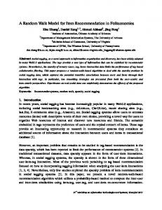
] p (1k) ~ r,t ! ] p (1k) ~ r,t ! 52 v 2lp (1k) ~ r,t ! 1l b p (2k) ~ r,t ! ]t ]xk FIG. 1. Sample of the trajectory of a photon inside the slab. Note the situation of the axes.
our model are addressed in Sec. V. Conclusions are drawn in Sec. VI. II. THREE-DIMENSIONAL PERSISTENT RANDOM WALK IN THE SLAB
We consider the infinite slab of thickness L. The physical picture behind the random walk theory for multiple scattering transport is that photons move between collisions in a straight line at a constant velocity v that is characteristic of the medium. The scattering events change the direction in which photons are traveling but not the magnitude of the velocity v . The number of collisions follow a Poisson law of rate l. In this way, the mean time between two consecutive scattering events is l 21 , or equivalently, the scattering mean free path is l s 5 v l 21 . We show below that absorption can be easily introduced in this formulation but we do not consider it for the moment. The last magnitude required to characterize the model is the phase function f ( g ), which provides the probability density function of the relative angle between the photon direction of motion before and after a collision. In our model, this function reads f ~ g ! 5 ~ 12 b ! d ~ g 2 p /2! 1 b d ~ g 2 p ! ,
~2.1!
with the additional limitation that among the orthogonal directions only the four parallel to the axes X, Y, or Z are possible. In other words, after a collision photons will either reverse their previous direction with probability b or turn to one of the four possible orthogonal directions with probability (12 b )/4 each. Figure 1 shows a realization of a photon path between the two faces of the slab at the planes x50 and x5L according to our model. Forward scattering is incorporated automatically in the model by the definition of l because a forward collision is completely equivalent to straight motion. In the Appendix, we explain how to rescale l and the scattering probabilities in order to work with a phase function with no forward scattering as Eq. ~2.1!. The local anisotropy of the scattering is quantified by the average value of the cosine of the scattering angle, g5 ^ cos g&. In our case,
1 1 l ~ 12 b ! @ p (1 j) ~ r,t ! 1 p (2 j) ~ r,t !# , 4 jÞk
(
~2.3!
] p (2k) ~ r,t ! ] p (2k) ~ r,t ! 5v 2lp (2k) ~ r,t ! 1l b p (1k) ~ r,t ! ]t ]xk 1 1 l ~ 12 b ! @ p (1 j) ~ r,t ! 1 p (2 j) ~ r,t !# 4 jÞk
(
~2.4! (k51,2,3). Let us now specify the initial and boundary conditions that are necessary to solve this set of equations. We assume that the x axis is orthogonal to the slab sides as shown in Fig. 1. Thus boundary conditions are p (11) ~ x50,y,z;t ! 5 p (21) ~ x5L,y,z;t ! 50,
~2.5!
which take into account that any particle cannot enter the slab from outside. Internal reflection due to optical index mismatch at the slab surfaces is not considered although it might be incorporated by changing the boundary conditions. We must have some care in handling the initial conditions since photons are injected at x50 into the slab and this initial condition is in contradiction with boundary condition ~2.5! when t50. To avoid such a problem we assume that photons are injected inside the slab at a depth x 0 and take the limit x 0 →0 1 at the end of the calculations. Consequently, the initial conditions are p (11) ~ x,y,z;0 ! 5 d ~ x2x 0 ! d ~ y ! d ~ z ! ,
~2.6!
p (21) ~ x,y,z;0 ! 5 p (62) ~ x,y,z;0 ! 5 p (63) ~ x,y,z;0 ! 50. ~2.7! In what follows we will work with dimensionless variables defined by t 8 5lt,
r8 5lr/ v ,
~2.8!
and for notational convenience we drop primes hereafter. Note that this scaling is equivalent to setting v 51 and l 51 in the above equations; in other words, we measure time
PRE 59
PERSISTENT RANDOM WALK MODEL FOR TRANSPORT . . .
in units of the mean time between collisions l 21 and length in units of the scattering mean free path l s 5 v l 21 . The solution to the problem posed by Eqs. ~2.3!–~2.7! is easily obtained by using the following joint two-dimensional Fourier and Laplace transform: ˜p ~ x, v;s ! 5
E
`
2`
dye 2i v 2 y
E
`
2`
dze 2i v 3 z
E
`
0
where v5( v 2 , v 3 ). From the joint transformation of system ~2.3!–~2.4! for k52,3, we get the algebraic relation
(
jÞ1
˜p (11) ~ x ! 5 ~ m 2h ! Ae 2 m x 2 ~ m 1h ! Be m x ,
~2.16!
˜p (21) ~ x ! 5c @ Ae 2 m x 1Be m x # ,
~2.17!
where h and c where defined in Eq. ~2.15! and m 5 m ( v;s) is given by
dte 2st p ~ r;t ! , ~2.9!
m 5 Ah 2 2c 2 .
A5
˜ (21) ~ x, v;s !# , 52F ~ v;s !@ ˜p (11) ~ x, v;s ! 1p
H
~ m 1h ! x ~ L2x 0 ! / ~ m 2h ! ,
e
2mL
~2.10! B5
where f ~ v 2 ;s ! 1 f ~ v 3 ;s ! 1 f ~ v 2 ;s ! f ~ v 3 ;s ! 42 f ~ v 2 ;s ! f ~ v 3 ;s !
~ 12 b !@ s1 ~ 11 b !# @ s1 ~ 12 b !#@ s1 ~ 11 b !# 1 v
. 2
~2.11!
~2.12!
The variable v 2 is the modulus of vector v. The substitution of Eq. ~2.10! into Eqs. ~2.3! and ~2.4! ~with k51) results in ˜ (61) (x, v;s): the following set of equations for ˜p (61) (x)[p ˜ (11) ~ x ! dp ˜ (11) ~ x ! 2c ˜p (21) ~ x ! 5 d ~ x2x 0 ! , 2hp dx ˜ (21) ~ x ! dp ˜ (21) ~ x ! 1c ˜p (11) ~ x ! 50, 1hp dx
H
@~ 1/2m ! e
2mx0
x,x 0 ,
2 x ~ L2x 0 !# ,
x ~ L2x 0 ! ,
x.x 0 ,
x,x 0 ,
x ~ L2x 0 ! 2 ~ 1/2m ! e
2mx0
,
x.x 0 ,
~2.19! ~2.20!
where
x~ x ![
and f ~ v;s ! [
~2.18!
The quantities A j and B j ( j51,2) can be found from the boundary conditions at x50 and x5L and from the discontinuity, due to the initial condition, of the densities ˜p 61 (x) at the photon injection point x 0 . After some algebra we obtain
˜ (2 j) ~ x, v;s !# @ ˜p (1 j) ~ x, v;s ! 1p
F ~ v;s ! [
6519
~2.13! ~2.14!
where h5h( v;s) and c5c( v;s) are defined by
~ m 2h ! sinh m x . 2 m @ m cosh m L2h sinh m L #
~2.21!
Equations ~2.16!–~2.21! furnish the complete solution to our problem. In those cases where particles are injected on the surface of the slab, the exact solution can be simplified after taking the limit x 0 →0 1 in the expressions above. In this case we have ˜p (11) ~ x ! 5
F
G
1 2 x ~ L ! @~ m 2h ! e 2 m (L2x) 1 ~ m 1h ! e m x # , 2m ~2.22!
˜p (21) ~ x ! 5c
F
G
1 2 x ~ L ! @ e 2 m x 1e m x # . 2m
~2.23!
In most situations, one is interested in photon concentration regardless of photon velocity. The total probability density p(r,t) for the position independent of the velocity reads 3
p ~ r;t ! 5
1 h[ ~ 12 b ! F ~ v;s ! 2 ~ s11 ! , 2 1 c[ ~ 12 b ! F ~ v;s ! 1 b . 2
~2.15!
We have thus turned the original problem ~2.3!–~2.7! into the simpler problem given by Eqs. ~2.13! and ~2.14! and boundary conditions ~2.5!. Note that we have actually reduced the transport problem through a three-dimensional slab to a one-dimensional problem which is very similar to the problem of solving the one-dimensional telegrapher’s equation in the presence of traps, a problem we successfully addressed some time ago @18,19#. The exact solution to Eqs. ~2.13! and ~2.14! along with Eq. ~2.5! is straightforwardly obtained and the solution can be written as
(
k51
@ p (1k) ~ r;t ! 1 p (2k) ~ r;t !# .
~2.24!
It was mentioned above that absorption can be readily introduced in our formulation. Indeed, if photons can be absorbed at any point of the medium at a constant rate l a independent of the position and direction of photon motion, then it is enough to multiply all densities by the factor exp(2lat) @4# to incorporate absorption. Thus, for instance, the total density ~2.24! will be p a ~ r;t ! 5e 2l a t p ~ r;t ! .
~2.25!
In the Laplace domain, the relation between quantities when there is or not absorption becomes particularly simple, since in this case we have pˆ a ~ r;s ! 5 pˆ ~ r;l a 1s ! ,
~2.26!
˜A ´ , PORRA ` , AND MASOLIVER BOGUN
6520
where pˆ a (r;s) is the Laplace transform of the total probability density function.
where pˆ (r;s1l a ) is the Laplace transform of the nonabsorbing total probability density. In terms of the joint FourierLaplace transform defined in Eq. ~2.9! we have
III. SURVIVAL PROBABILITY: CHARACTERISTIC TIMES
We now use the exact solution, Eqs. ~2.22! and ~2.23!, obtained in the previous section to calculate several characteristic times of photon motion that are relevant for timeresolved experiments. To this end we will first evaluate the survival probability S(t), which is the probability the particle is still inside the slab at time t. In terms of the total probability density function in the presence of traps, p(r;t), which we have just obtained above, the survival probability can be evaluated by @4# S~ t !5
E E E `
L
dx
2`
0
dy
`
2`
E E E `
L
dx
0
Sˆ a ~ s ! 5
2`
dy
`
2`
~3.2!
pˆ ~ r;s1l a ! dz,
E
L
qˆ ~ x;s1l a ! dx,
~3.3!
qˆ ~ x;s ! [ ˜p ~ x, v;s ! u v5(0,0) .
~3.4!
0
where
Moreover, we see from Eqs. ~2.10! and ~2.24! that Sˆ a ~ s ! 5 @ 112F ~ s !#
E
L
0
@ qˆ (11) ~ x,s ! 1qˆ (21) ~ x,s !# dx,
~3.5!
where qˆ (61) (x,s) is defined as in Eq. ~3.4! with ˜p (x, v;s) replaced by the density ˜p (61) (x, v;s). Function F(s) is simply F( v;s), Eq. ~2.11!, at v5(0,0), F ~ s ! [F ~ v;s ! u v5(0,0) .
~3.6!
The substitution of Eqs. ~2.16! and ~2.17! into Eq. ~3.5! yields
2 @ h a cosh m a ~ L1x 0 ! /22 m a sinh m a ~ L1x 0 ! /2# sinh m a ~ L2x 0 ! /21c a sinh m a ~ L2x 0 ! , ~ s1l a !@ h a sinh m a L2 m a cosh m a L #
1 h a 5 ~ 12 b ! F ~ l a 1s ! 2 ~ l a 1s11 ! , 2 1 c a 5 ~ 12 b ! F ~ l a 1s ! 1 b , 2
~3.8!
m a5 A
h 2a 2c 2a .
Knowledge of Sˆ a (s) allows us to obtain the mean residence time ^ T a & of photons inside the slab. Note that the residence time T a coincides in the absence of absorption with the escape time out of the slab. The residence time moments will be given, in terms of the Laplace transform Sˆ a (s), by
t n ~ L,l a ! 5 ~ 21 ! n21 n
d n21 Sˆ a ~ s ! ds n21
U
~3.7!
where h 0 , c 0 , and m 0 , are given by Eq. ~3.8! after setting s 50, that is,
where @cf. Eqs. ~2.15!, ~2.18! and Eq. ~3.6!#
~3.9!
. s50
The mean residence time is thus given by t 1 5 ^ T a & 5Sˆ a (0). From now on we will assume that photons are initially injected on the surface of the slab and therefore x 0 50 1 . From Eqs. ~2.22!, ~2.23!, and ~3.5! we get
F
Sˆ a ~ s ! 5
~3.1!
p ~ r;t ! dz.
In what follows we assume that we deal with an absorbing medium of rate l a . We denote by S a (t) the survival probability in the presence of absorption; its Laplace transform is given by @cf. Eqs ~2.25! and ~2.26!# Sˆ a ~ s ! 5
PRE 59
G
m 0 1c 0 sinh m 0 L 1 t 1 ~ L,l a ! 5 12 , la m 0 cosh m 0 L2h 0 sinh m 0 L
1 h 0 5 ~ 12 b ! F ~ l a ! 2 ~ l a 11 ! , 2 1 c 0 5 ~ 12 b ! F ~ l a ! 1 b , 2
The behavior of the mean residence time depends on whether the slab thickness L is less or greater than a critical value defined by L c5
1 . m0
~3.12!
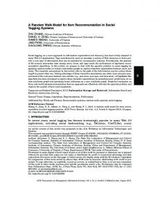
In Fig. 2, the mean residence time, Eq. ~3.10!, is plotted as a function of the slab thickness L. As in many experimental settings @14#, we will assume in what follows that the isotropization length l iso is much shorter than the absorption 21 length, i.e., l a 5 v l 21 /(11 b ). In this case @see a @l iso5 v l Eq. ~3.11!#, the factor m 0 can be approximated as follows:
m 0; ~3.10!
m 05 A
~3.11!
h 20 2c 20 .
A
3 1O ~ l iso /l a ! , l a l iso
and the critical thickness is given by
~3.13!
PERSISTENT RANDOM WALK MODEL FOR TRANSPORT . . .
PRE 59
6521
L lim t 1 ~ L,l a ! 5 ^ T & 53 . v l a →0
~3.17!
The mean escape time in this limit is 3 times as much as the ballistic time to cross the slab. This is somewhat surprising since one would expect that, as L→0, the escape time should approach the ballistic time, t 1 ;L/ v . Nevertheless, one can show that this longer time is due to those particles which, after the first collision, remain moving parallel to the slab faces. Indeed, we first note that the average time that takes a particle moving in a plane parallel to the slab faces to leave such a plane is T Y Z5 FIG. 2. Mean escape time t 1 (L,l a ) in l 21 units as a function of slab size L in l5 v /l units. The values of the absorption rate l a are l a 50.1l ~solid line!, l a 50.05l ~dotted line!, l a 50.033l ~short dashed line!, and l a 50.025l ~long dashed line!. In this figure, b 50.5 and x 0 50 1 .
L c ' Al a l iso/3.
~3.14!
Note that we have reintroduced units, Eq. ~2.8!, in this discussion. If no absorption exists, l a 50 and l a 5L c 5`, while if l a 5`, then l a 5L c 50. Therefore, for thin slabs where L!L c absorption is negligible, but for thick slabs where L @L c , the medium is strongly absorbing. We also note that in our simplified model for transport the condition for neglecting absorption does not simply consist in comparing slab thickness L with the absorption length l a , but to compare L with L c , that is, with the square root of l a . Hence, the size L for which one does not have to take into account absorption is less than one might think a priori. Whether this observation is a particular feature of our model, due to the fact that particles can move parallel to slab faces without any bound ~see below!, or it is a general property will be investigated further. The absorbing and nonabsorbing regimes can be clearly seen from the asymptotic behavior of the mean residence time as a function of slab thickness L ~see Fig. 2!. Thus, from Eq. ~3.10! it follows that in the limit of high absorption and L@L c , the escape time approaches a constant value independent of slab thickness:
t 1 ~ L,l a ! 5
F
G
1 c0 11 1O ~ e 2L/L c ! . la h 02 m 0
~3.15!
The values of c 0 , h 0 , and m 0 are those given in Eq. ~3.11! but with units. For instance, coefficient c 0 reads c 0 5l(1 2 b )F(l a /l)/(2 v )1l b / v and has dimensions of @ L 21 # . In the low-absorption limit, assuming that L!L c , we can see from Eq. ~3.10! that 2l a 13 ~ 12 b ! l L t 1 ~ L,l a ! ; . 2l a 1 ~ 12 b ! l v
~3.16!
In the limit l a →0 when no absorption is present, we have
2 . l ~ 12 b !
~3.18!
This result is readily obtained by taking into account that after a collision there is a probability b 1(12 b )/2 that such a particle does not leave the plane. When L→0, the main contribution to the escape time comes from those particles that do not suffer any collision and therefore take a time L/ v to cross the slab. The probability that a particle is not scattered is exp(2lt) which is approximately 12lL/ v when L →0. However, those particles that are scattered in a direction parallel to the slab faces add to the escape time twice as much as the first ones. The probability that a particle suffers a collision that brings it to move in such a direction is the scattering probability 12exp(2lt);lL/v times the probability, 12 b , to be scattered in the right direction. Therefore, the escape time when L→0 reads T esc;
S
D
L L L L 12l 1l ~ 12 b ! T Y Z 1O ~ L 2 ! 53 , v v v v ~3.19!
where we have used Eq. ~3.18!. In fact, the transmission time @13# is the average time usually measured in time-resolved experiments instead of the escape time given above. The transmission time is the mean of the time that takes a photon to leave the slab through the opposite face to that it was injected. We will evaluate the transmission time when absorption is negligible, although by a straightforward but lengthy calculation one can also deal with the absorbing case. In what follows we use again the dimensionless variables given by Eq. ~2.8!. Let us denote by J tr(t) the flux of particles leaving the slab through the opposite face of the entering one. The probability density function of the transmission time p tr(t) is then given by p tr~ t ! 5
J tr~ t !
.
~3.20!
dz p (11) ~ x5L,y,z;t ! ,
~3.21!
E
`
0
J tr~ t ! dt
In our case, the flux reads J tr~ t ! 5 v
E E `
2`
dy
`
2`
where v 51 since we are using dimensionless units. The Laplace transform of p tr(t) is
˜A ´ , PORRA ` , AND MASOLIVER BOGUN
6522
qˆ (11) ~ L,s ! , qˆ (11) ~ L,0!
pˆ tr~ s ! 5
PRE 59
~3.22!
where ˜ (11) ~ x, v;s ! u v5(0,0) . qˆ (11) ~ x;s ! [p
~3.23!
In terms of pˆ tr(s), the mean transmission time
t tr~ L ! 52
dpˆ tr~ s ! ds
U
~3.24! s50
can be calculated from Eq. ~2.22! and is
S
t tr~ L ! 5L 21
D
L . 2l iso
~3.25!
In the limit L!l iso , the transmission time is t tr(L);2L, which is twice as much as the ballistic time to cross the slab. As in the case of the escape time, this is again due to those particles moving parallel to the slab sides. We mention that this anomalous effect of a lack of convergence of characteristic times to the ballistic time when L→0 has been reported for other transport models although for higher-order moments only @20#. For a thick slab L/l iso@1 and the transmission time becomes in dimensionless units, Eq. ~2.8!, L2 t tr~ L ! ; 2l iso
FIG. 3. Stationary concentration of particles r a (x u x 0 ) ~in l 21 5l/ v units! inside the slab for b 50.5, n 0 5l, L510v /l, x 0 5 v /l, and l a 50.1l ~dotted line!, l a 50.04l ~short dashed line!, l a 50.025l ~long dashed line!, and l a 50 ~solid line!. Position x is plotted in l5 v /l units
where F(s) is given by Eq. ~3.6!, and qˆ (6) (x,s) is defined by Eq. ~3.4!. Now the substitution of Eqs. ~2.16! and ~2.17! into Eq. ~4.2! yields
r a ~ x u x 0 ! 5G 1 @~ h 0 2c 0 ! sinh m 0 x2 m 0 cosh m 0 x #
~3.26!
or, after reintroducing units,
~4.3!
~ x,x 0 !
and
t tr~ L ! ;
L2 . 2 v l iso
r a ~ x u x 0 ! 5G 2 @~ h 0 2c 0 ! sinh m 0 ~ L2x !
~3.27!
This result agrees with that obtained from the diffusion approximation although we postpone the discussion about the diffusion approximation to Sec. VI. The transition between the ballistic and diffusive regimes occurs when L;5l iso .
2 m 0 cosh m 0 ~ L2x !#
~ x.x 0 ! ,
where G 1 5n 0
c 0 @ 2l a 13 ~ 12 b !# sinh m 0 ~ L2x 0 ! ] , m 0 @ 2l a 1 ~ 12 b !#@ h 0 sinh m 0 L2 m 0 cosh m 0 L # ~4.5!
IV. STATIONARY PROPERTIES
In this section we study the stationary properties of the model that are relevant in cw experiments. Specifically we will first obtain the stationary particle concentration inside the slab. We assume that photons are continuously injected at a rate n 0 , all of them moving to the right, at the initial point x 0 @21#. Absorption is also considered at a constant rate l a . Let r a (x u x 0 ) be the stationary particle concentration inside the slab. In terms of the total probability density function p(x,y,z;t) of a point source at x 0 @cf. Eq. ~2.24!# we have
r a ~ x u x 0 ! 5n 0
E E E `
2`
`
dy
2`
`
dz
0
~4.4!
dte 2l a t p ~ x,y,z;t ! . ~4.1!
Using Eq. ~2.10!, we get
r a ~ x u x 0 ! 5n 0 @ 112F ~ l a !#@ qˆ (11) ~ x,l a ! 1qˆ (21) ~ x,l a !# , ~4.2!
G 2 5n 0
@ 2l a 13 ~ 12 b !#@ m 0 cosh m 0 x 0 2h 0 sinh m 0 x 0 # , m 0 @ 2l a 1 ~ 12 b !#@ h 0 sinh m 0 L2 m 0 cosh m 0 L #
~4.6! and h 0 , c 0 , and m 0 are given by Eq. ~3.11!. We note that the escape time t 1 (L,l a ), Eq. ~3.10!, can also be obtained in terms of r a (x u x 0 ) using the flux over population method as @22,23#
t 1 ~ L,l a ! 5
1 n0
Er L
0
a ~ x u x 0 ! dx.
~4.7!
In Fig. 3, we plot r a (x u x 0 ) for several values of the absorbing rate l a . For finite values of l a the concentration profile decays exponentially while in the absence of absorption we have the linear behavior:
r ~ x u x 0 ! 5n 0
3 ~ L2x 0 !~ l iso1x ! l iso~ 2l iso1L !
~ x,x 0 ! ,
~4.8!
PERSISTENT RANDOM WALK MODEL FOR TRANSPORT . . .
PRE 59
6523
and
r ~ x u x 0 ! 5n 0
3 ~ 2l iso1x 0 !~ l iso1L2x ! l iso~ 2l iso1L !
~ x.x 0 ! .
~4.9!
The discontinuity of r (x u x 0 ) at x5x 0 is simply a consequence of the injection of particles with positive velocity. This discontinuous behavior is a general feature of any model where particles have finite velocity, and it has also been observed in models using the telegrapher’s equation as a transport equation @25#. We evaluate now a relevant quantity in transmissionwave spectroscopy: the transmission and reflection coefficients T(L,l a ) and R(L,l a ). As is well known, the transmission ~reflection! coefficient is related to the flux of particles that, being injected in one side, leave the slab from the opposite ~same! side. The transmission coefficient is the integral over all times of the transmitted flux J tr(t) and its expression is T ~ L,l a ! 5
E
5v
`
0
J tr~ t ! dt
E E E `
`
dt
0
2`
dy
`
2`
dze 2l a t p (11) ~ x5L,y,z;t ! , ~4.10!
where v 51 because of dimensionless units. When absorption is not considered, the definition of J tr(t) used in this expression is equivalent to Eq. ~3.21!. The reflection coefficient is defined analogously but taking the flux at x50. In our model, where fluxes are discrete, we have the simpler expressions in terms of the Laplace-Fourier transform of p (61) (x, v;s): T ~ L,l a ! 5 v ˜p (11) ~ L, v;l a ! u v5(0,0)
~4.11!
R ~ L,l a ! 5 v ˜p (21) ~ 0,v;l a ! u v5(0,0) ,
~4.12!
and
where v 51 because of dimensionless variables. Assuming that x 0 50 1 , we obtain from Eqs. ~2.22! and ~2.23! that T ~ L,l a ! 5
m0 m 0 cosh m 0 L2h 0 sinh m 0 L
~4.13!
and
FIG. 4. Transmission T and reflection R coefficients as a function of slab size L in l5 v /l units for b 50.5, x 0 50 1 and l a 5l ~solid line!, l a 50.1l ~dotted line!, l a 50.01l ~short dashed line!, and l a 50.001l ~long dashed line!. V. DIFFUSION APPROXIMATION
For the model proposed, we have been able to obtain all relevant quantities exactly. This is a rather exceptional case due to the peculiar form of the model phase function, Eq. ~2.1!. In general, most magnitudes have to be calculated within an approximation scheme. Among them, diffusion theory is the most often used in analyzing experimental results. By comparing our results with those given by the diffusion approximation, we can test how well this approach works with our model. This comparison will provide additional evidence about the limits of the diffusion approximation. In what follows, absorption is neglected because diffusion theory gives better results when there is no absorption @24#. The diffusion constant D that appears in the diffusive theory can be written as D5
R ~ L,l a ! 5
c 0 sinh m 0 L , m 0 cosh m 0 L2h 0 sinh m 0 L
~4.14!
In Fig. 4, we plot these functions for different absorption rates. Note that, due to absorption, R(L,l a )1T(L,l a )Þ1. In the absence of absorption, these coefficients reduce to T ~ L,0! 5
2l iso , 2l iso1L
R ~ L,0! 5
and obviously R(L,0)1T(L,0)51.
L , 2l iso1L
~4.15!
v l iso , 3
~5.1!
where v is the photon velocity inside the medium and l iso is the isotropization length defined in Sec. II. In addition to D, diffusion theory introduces two more parameters, the extrapolation length l e and the penetration length l p , to treat the boundary conditions and the source of photons, respectively. In terms of these parameters, the transmission coefficient predicted by diffusion theory is @25# T dif5
l p 1l e . L12l e
~5.2!
˜A ´ , PORRA ` , AND MASOLIVER BOGUN
6524
When L is large enough to disregard the ballistic photons ~those that cross the slab without being scattered!, T dif agrees with the transmission probability calculated for our model, Eq. ~4.15!, provided l p and l e are both equal to l iso . The penetration length obtained corresponds to the most used value. However, the extrapolation length differs from the standard value that follows from diffusion theory, l e 52l iso/3. The reason for this apparent disagreement is the limited number of velocity directions allowed by our model. Indeed, from the exact stationary probability density, Eqs. ~4.8! and ~4.9!, the extrapolation length calculated by the requirement
S
12l e
D
d r~ xux0! dx
U
50
~5.3!
x50
gives precisely l e 5l iso . A similar calculation yields the same value for the extrapolation length at the other slab face, when L is large enough to neglect the ballistic photons. Moreover, as the diffusive part of the stationary density becomes linear close to the slab sides, the extrapolation length can also be obtained in this case from the solution of r (2l e u x 0 )50. Once the lengths l e and l p are known, it is possible to use the diffusion approximation to calculate other quantities of interest. For instance, the escape time ^ T & can be obtained from the mean first-passage time of a free system driven by white noise and the result is L v
^ T & 53 ,
~5.4!
which coincides with the exact calculation given by Eq. ~3.17!. The transmission time can also be computed in the diffusion approximation @1#. In order to obtain it, we begin with the expression for the photon concentration in a slab with faces at x5l e and x5L1l e when a unit pulse is injected at x 0 5l e 1l p 52l e , 2 p ~ x,t ! 5 L12l e
F
`
mpx
mpx
( sin L12l0e sin L12l e m51
3exp 2
Dtm 2 p 2 ~ L12l e ! 2
G
.
~5.5!
Note that the latter expression vanishes at x50 and x5L 12l e which correspond to the extrapolated boundaries of the slab of width L located between x5l e and x5L1l e . The transmitted flux J dif reads J dif~ t ! 52D 5
d p ~ x,t ! u x5L1l e dx
PRE 59
Using this result, we obtain the average transmission time T tr given by the diffusion approximation, that is,
E E
`
T tr5
0
tJ dif~ t ! dt
`
0
5 J dif~ t ! dt
L 2 14Ll iso23l 2iso 2 v l iso
.
~5.7!
To derive this expression, we took into account that for our model l e 5l iso . In this case, the diffusion approximation is also very accurate because the exact result, Eq. ~3.25!, and T tr differ only by a constant factor 23l iso/2. Therefore, the diffusion approximation works for our model well below the accepted limit of failure of such approach for more realistic models @13#. As we have explained, this is a consequence of the limited number of photon directions of motion allowed by the model.
VI. CONCLUSIONS
In this paper we have proposed a model for light propagation through a thin slab. The main property of the model is that photons can only take a restricted set of velocity directions. This limitation has the advantage that has allowed us to compute most relevant properties in experimental studies without any approximation. Among the interesting quantities in multiple light scattering experiments, we have concentrated on the properties of the transmitted flux. In most calculations, absorption has been taken into account. In particular, we have shown its influence in the mean survival time of photon inside the slab. Our exact calculations have been compared with those obtained from the diffusion approximation, the most widely used approach in the analysis of multiple light scattering data. We were able to obtain the exact expression for the extrapolated length. Using this parameter, the results of the diffusion approximation agree very well with the exact ones even below the region where it is known from experiments that the diffusion approximation does not work. The reason for this agreement lies on the limited number of directions along which photons can move. However, the model is really three dimensional as reflected by the diffusion constant associated with it. The diffusion approximation cannot give, however, the discontinuity in the stationary density at the position of photon injection. This feature could be used to test other approximation schemes, like the use of a phenomenological telegrapher’s equation.
Dp ~ L12l e ! 2 `
3
(m m51
F
F
3exp 2
sin
m p ~ L2l e ! m p ~ L13l e ! 2sin L12l e L12l e
Dtm 2 p 2 ~ L12l e ! 2
G
.
G ~5.6!
ACKNOWLEDGMENTS
This work has been supported in part by Direccio´n General de Investigacio´n Cientı´fica y Te´cnica under Contract No. PB96-0188 and Project No. HB119-0104, and by Societat Catalana de Fı´sica ~Institut d’Estudis Catalans!.
PRE 59
PERSISTENT RANDOM WALK MODEL FOR TRANSPORT . . . APPENDIX: FORWARD SCATTERING
The model explained in Sec. II confines the directions of photon motion to those parallel to the axes X, Y, and Z. Due to this restriction, forward scattering cannot be distinguished from straight motion. This property allows us to rewrite the phase function in such a way that only takes into account those collisions that produce a change in motion direction ~including a reversion!, that is, with no forward scattering included. Indeed, let us assume a general phase function for our model: f 1 ~ g ! 5p f d ~ g ! 1p b d ~ g 2 p ! 1p o d ~ g 2 p /2! ,
p~ t !5
1
t8
exp~ 2t/ t 8 ! ,
ˆ (s), the Laplace transscattering event. The expression for U form of U(t), becomes simpler because the sum over k can be worked out: ˆ ~ s !5 U
t8 t 8 s11
~A2!
where t 8 is the average time between consecutive scattering events. The scattering mean free path is simply v t 8 . Let U(t) be the probability that the photon keeps moving in the same direction for a time greater than t. Using Eqs. ~A1! and ~A2! and taking into account that the result of a forward collision does not differ from straight motion, we see that U(t) is given by
`
1
( k51
p kf
t 8k ~ t 8 s11 !
5 k11
t8 t 8 s112p f
. ~A4!
ˆ (s) yields The Laplace inversion of U U ~ t ! 5exp~ 2t/ t ! ,
~A1!
where p f is the forward scattering probability, p b is the backscattering probability and p o gives the probability that after a collision a photon turns to any of the four orthogonal directions that are parallel to the axes X, Y, and Z. The time between two successive collisions is distributed according to the following exponential probability density function:
6525
~A5!
with a new parameter t :
t5
t8 . 12 p f
~A6!
Therefore, times between scattering events that produce a change in motion direction are also exponentially distributed with an average time between collisions equal to t . After one of these events, a photon can only move in an orthogonal direction ( g 5 p /2) or reverse its direction of motion ( g 5 p ). Thus, the phase function can be written f ~ g !5
po pb d ~ g 2 p /2! 1 d~ g2p !, 12 p f 12 p f
~A7!
where P(t)5exp(2t/t8) is the survival probability and p k (t) is the probability density function for the time of the kth
which agrees with Eq. ~2.1! if b 5 p b /(12 p f ). It follows from this analysis that the forward scattering probability is incorporated in the model by rescaling the average time between scattering events as t 5 t 8 /(12p f ) and changing the phase function from Eq. ~A1! to Eq. ~2.1!. Note that the anisotropy factor g is always negative because forward scattering is included in the rescaled l5(12p f )l 8 and not in the phase function.
@1# B.B. Das, Feng Liu, and R.R. Alfano, Rep. Prog. Phys. 60, 227 ~1997!. @2# Optical Tomography, Photon Migration, and Spectroscopy of Tissue and Model Media, edited by B. Chance and R.R. Alfano, Proc. SPIE No. 2389 ~SPIE, Bellingham, 1995!; bibliography in Trends in Optics and Photonics, TOPS Vol II, edited by R.R. Alfano and J.G. Fujimoto ~Optical Society of America, Washington, D.C., 1996!. @3# Laser-Doppler Blood Flowmetry, edited by A.P. Shepherd and P.A. Oberg ~Luwer, Boston, 1990!. @4# G.H. Weiss, Aspects and Applications of the Random Walk ~North-Holland, Amsterdam, 1994!. @5# A. Ishimaru, Wave Propagation and Scattering in Random Media ~Academic, New York, 1978!, Vol. I; Appl. Opt. 28, 2210 ~1989!. @6# R.F. Bonner, R. Nossal, S. Havlin, and G.H. Weiss, J. Opt. Soc. Am. A 4, 423 ~1987!. @7# A.H. Gandjbakhche and G.H. Weiss, Prog. Opt. 34, 333 ~1995!.
@8# J.M. Porra`, J. Masoliver, and G.H. Weiss, Phys. Rev. E 55, 7771 ~1997!. @9# D.J. Durian and J. Rudnick, J. Opt. Soc. Am. A 14, 235 ~1997!. @10# A.H. Gandjbakhche, R.F. Bonner, and R. Nossal, J. Stat. Phys. 69, 35 ~1992!. @11# A.H. Gandjbakhche, R. Nossal, and R.F. Bonner, Appl. Opt. 32, 504 ~1993!. @12# D.J. Durian, Phys. Rev. E 50, 857 ~1994!. @13# K.M. Yoo, Feng Liu, and R.R. Alfano, Phys. Rev. Lett. 64, 2647 ~1990!. @14# R.H.J. Kop, P. de Vries, R. Sprik, and A. Lagendijk, Phys. Rev. Lett. 79, 4369 ~1997!. ˜ a´, J.M. Porra`, and J. Masoliver, Phys. Rev. E 58, @15# M. Bogun 6992 ~1998!. @16# I. Claes and C. Van den Broeck, J. Stat. Phys. 49, 383 ~1987!. @17# S. Goldstein, Q. J. Mech. Appl. Math. 4, 129 ~1951!. @18# J. Masoliver, J.M. Porra`, and G.H. Weiss, Phys. Rev. A 45, 2222 ~1992!. @19# J. Masoliver, J.M. Porra`, and G.H. Weiss, Phys. Rev. E 48, 939 ~1992!.
( p kf E0 P ~ t2t 8 ! p k~ t 8 ! dt 8 , k51 `
U~ t !5 P~ t !1
t
~A3!
6526
˜A ´ , PORRA ` , AND MASOLIVER BOGUN
@20# C.R. Doering, T.S. Ray, and M.L. Glasser, Phys. Rev. A 45, 825 ~1992!; T.S. Ray, M.L. Glasser, and C.R. Doering, ibid. 45, 8573 ~1992!. @21# G.H. Weiss, R. Nossal, and R.F. Bonner, J. Mod. Opt. 36, 349 ~1989!. @22# L. Farkas, Z. Phys. Chem. ~Leipzig! 125, 236 ~1927!.
PRE 59
@23# P. Ha¨nggi, P. Talkner, and M. Borkovec, Rev. Mod. Phys. 62, 251 ~1990!. @24# J. J. Duderstand and W. R. Martin, Transport Theory ~Wiley, New York, 1979!. @25# P.A. Lemieux, M.U. Vera, and D.J. Durian, Phys. Rev. E 57, 4498 ~1998!.