Phase transitions in optimal unsupervised learning

PHYSICAL REVIEW E

VOLUME 57, NUMBER 3

MARCH 1998

Phase transitions in optimal unsupervised learning Arnaud Buhot and Mirta B. Gordon* De´partement de Recherche Fondamentale sur la Matie`re Condense´e, CEA/Grenoble, 17 rue des Martyrs, 38054 Grenoble Cedex 9, France ~Received 25 September 1997; revised manuscript received 12 November 1997! We determine the optimal performance of learning the orientation of the symmetry axis of a set of P 5 a N points that are uniformly distributed in all the directions but one on the N-dimensional space. The components along the symmetry breaking direction, of unitary vector B, are sampled from a mixture of two Gaussians of variable separation and width. The typical optimal performance is measured through the overlap R opt5B•J* , where J* is the optimal guess of the symmetry breaking direction. Within this general scenario, the learning curves R opt( a ) may present first order transitions if the clusters are narrow enough. Close to these transitions, high performance states can be obtained through the minimization of the corresponding optimal potential, although these solutions are metastable, and therefore not learnable, within the usual Bayesian scenario. @S1063-651X~98!07303-6# PACS number~s!: 87.10.1e, 02.50.2r, 05.20.2y

I. INTRODUCTION

In this paper we address a very general problem in the statistical analysis of large amounts of data points, also called examples, patterns, or training set, namely the problem of discovering the structure underlying the data set. Whether this determination is possible or not depends on the assumptions one is willing to accept @1#. Several algorithms allowing to detect structure in a set of points exist. Among them, principal component analysis finds the directions of higher variance, projection pursuit methods @2# seek directions in input space onto which the projections of the data maximize some measure of departure from normality, whereas self-organizing clustering procedures @3# allow to determine prototype vectors representative of clouds of data. The parametric approach assumes that the structure of the probability density function from which the patterns have been sampled is known. Only its parameters have to be determined given the examples. A frequent guess is that the probability density is either Gaussian or a mixture of Gaussians. The process of determining the corresponding parameters is called unsupervised learning, because we are not given any additional information about the data, in contrast with supervised learning, in which each training example is labeled. It has recently been shown that finding the principal component of a set of examples, clustering data with a mixture of Gaussians, and learning pattern classification from examples with neural networks may be cast as particular cases of unsupervised learning @4#. In all these problems, the examples are drawn from a probability density function ~PDF! with axial symmetry, and the symmetry-breaking direction has to be determined given the training set. As this direction may be found through the minimization of a cost function, the properties of unsupervised learning may be analyzed with statistical mechanics. This approach allows to establish the properties of the typical solution, determined in the thermodynamic limit, i.e., the space dimension N→1`, the num-

*Also at Centre National de la Recherche Scientifique. 1063-651X/98/57~3!/3326~8!/$15.00

57

ber of examples P→1`, with the fraction of examples a 5 P/N constant. Besides these general results, the statistical mechanics framework allows to deduce the expression of an optimal cost function @5–7#, whose minimum is the best solution that may be expected to be learned given the data. The optimal cost function depends on the functional structure of the PDF from which the examples are sampled, and on the fraction a of available examples. Its main interest is that it allows to deduce the upper bound for the typical performance that may be expected from any learning algorithm. On the other hand, Bayes’ formula of statistical inference allows to determine the probability of the symmetry-breaking direction given the training set. Sampling the direction with Bayes probability is called Gibbs learning @8#. The average of the solutions obtained through Gibbs learning, weighted with the corresponding probability, is called the Bayesian solution. It is widely believed that the Bayesian solution is optimal. Moreover, this has been so in all the scenarios considered so far. In the present paper, we consider a very general twocluster scenario, which contains results already reported as particular cases. In fact, two different situations, in which the pattern distribution is a Gaussian of zero mean and unit variance in all the directions but one, have been considered so far: a Gaussian scenario @9# and a two-cluster scenario @10,11,8#. In the former, the components of the examples parallel to the symmetry-breaking direction are sampled from a single Gaussian. In the latter these components are drawn from a mixture of two Gaussians, each one having unit variance. The learning process has to detect differences between the PDF along the symmetry-breaking direction and the distributions in the orthogonal directions. Several ad hoc cost functions allowing to determine the symmetry-breaking direction have been analyzed for both scenarios. Typically, if the PDF has a nonzero mean value in the symmetry-breaking direction, learning is ‘‘easy’’: the quality of the solution increases monotonically with the fraction a of examples, starting at a 50. In contrast, if the PDF has zero mean, the deviations of the PDF along the symmetry-breaking direction from the PDF in the orthogonal directions depend on the 3326

© 1998 The American Physical Society

57

PHASE TRANSITIONS IN OPTIMAL UNSUPERVISED . . .

second and higher moments. In this case, a phenomenon called retarded learning @8# appears: learning the symmetrybreaking direction becomes impossible when the fraction of examples falls below a critical value a c . Since we have considered the case of clusters of variable width, we could determine the entire phase diagram of the two-cluster scenario. Several new learning phases appear, depending on the mean and the variance of the clusters. In particular, if the second moment of the individual clusters is smaller than the second moment of the PDF in the orthogonal directions, first order transitions from low to high performance learning may occur as a function of a . Close to these, high performance metastable states exist above the stable states of Gibbs learning, in the thermodynamic limit. One of the most striking results of this paper is that these high performance metastable states can indeed be learned through the minimization of an optimal a -dependent potential, although they cannot be obtained through Bayesian learning. Our results have been obtained within the replica approach with the replica-symmetry hypothesis. We show below that this assumption is equivalent to the more intuitive requirement that the optimal learning curves R opt( a ) are increasing functions of the fraction of examples a . To our knowledge, this fact has not been noticed before. The paper is organized as follows. A short presentation of the problem and the replica calculation are given in Sec. II. In Sec. III we deduce the optimal cost functions within the replica-symmetry hypothesis, as well as the condition of replica-symmetry stability. In Sec. IV we deduce and discuss the optimal learning curves for the general two-cluster scenario. The typical properties of the optimal cost functions in the complete range of a , presented in Sec. V, show that Bayesian learning may not be optimal. Finally, the complete phase diagram is described in Sec. VI, as a function of the two clusters’ parameters. II. GENERAL FRAMEWORK AND REPLICA CALCULATION

We consider the general case of N-dimensional vectors j, the patterns or examples of the training set, drawn from an axially symmetric probability density P * ( j u B) of the form P * ~ j u B! [

1 ~2p!

N/2

H

J

j• j 2V * ~ l ! , exp 2 2

1

A2 p

H

exp 2

J

l2 2V * ~ l ! . 2

1`

2`

Dl exp@ 2V * ~ l !# 51,

~3!

where Dl5exp(2l2/2)dl/ A2 p . The different moments ^ l n & of ~2! are

^ l n& [

E

~ j•B! n P * ~ j u B! d j5

E

1`

2`

l n P * ~ l ! dl. ~4!

Several examples of functions V * have been treated in the literature so far @4,7–11#. In the particular case of supervised learning of a linearly separable classification task by a single unit neural network, the symmetry-breaking direction B is the teacher’s vector, orthogonal to the hyperplane separating the classes. The class of pattern j is t [sgn(B• j). The corresponding PDF is P * ( t l)52 Q( t l)exp(2l2/2)/ A2 p , i.e., V * (l)52ln2 for t l.0 and 1` for t l,0. In the following, we concentrate on the problem of unsupervised learning. We are given a training set La 5 $ jm % m 51, . . . , P of P5 a N vectors sampled independently with probability density P * ( j u B). We have to learn the unknown symmetry-breaking direction B from the examples knowing the functional dependence of P * on B. Using Bayes’ rule of inference, the probability of a direction J ~with J•J51) given the data is P ~ Ju La ! 5

1 Z

)m exp$ 2 jm • jm /22V *~ jm •J! % P 0~ J! ,

~5!

where P 0 (J)5 d (J•J21) is the assumed prior probability and Z5 * dJ) m exp$2jm • jm /22V * ( jm •J) % P 0 (J) is the probability of the training set. By analogy with supervised learning, sampling the direction with probability ~5! is called Gibbs learning @8#. We consider learning procedures where the direction J is found through the minimization of a cost function or energy E(J;La ). As the patterns are independently drawn, this energy is an additive function of the examples. The contribution of each pattern jm to E is given by a potential V that depends on the direction J and on jm through the projection ~called local field! g m 5J• jm : P

~1!

where B is a unitary vector in the symmetry-breaking direction, i.e., B•B51 ~notice that this is not the usual convention!, and l[ j•B5 ( i j i B i . According to Eq. ~1!, the patterns have normal distributions, i.e., P(x) 5exp(2x2/2)/ A2 p onto the N21 directions orthogonal to B. The distribution ~1! in the symmetry-breaking direction is P *~ l ! 5

E

3327

~2!

Thus, V * (l) introduces a modulation parallel to B; if V * 50 the patterns’ distribution is normal in all the directions. Normalization of P * requires

E ~ J;La ! 5

(

m 51

V~ gm!.

~6!

As the training set only carries partial information on the symmetry-breaking direction B, the direction J determined by the minimization of Eq. ~6! will generally differ from B. The quality of a solution J may be characterized by the overlap R5B•J. If R50, J does not give any information about the symmetry-breaking direction. Conversely, if R51 the symmetry-breaking direction is perfectly determined. The statistical mechanics approach allows to calculate the expected overlap R( a ) for any general distribution V * and any general potential V, in the thermodynamic limit N, P→ 1` with a [ P/N finite. In this limit, we expect that the energy is self-averaging: its distribution is a d peak centered at its expectation value independently of the particular realization of the training patterns. Given the modulation V * , different values of R may be reached, depending on the po-

3328

ARNAUD BUHOT AND MIRTA B. GORDON

tential used for learning. In the following, we sketch the main lines that allow to derive the typical value of R corresponding to a general potential V. The free energy F corresponding to the energy ~6! with a given potential V( g ) is

12R 2 5 a

R

1 F ~ b ,N,La ! 52 lnZ ~ b ,N,La ! , b

E

1`

2`

57

Dt @ g ~ t;c ! 2t # 2

A12R

2

5a

~7!

3

where b is the inverse temperature and Z the partition function: Z ~ b ,N,La ! 5

E

dJ exp$ 2 b E ~ J;La ! % d ~ J 21 ! . 2

~8!

As mentioned before, in the thermodynamic limit the free energy is self-averaging, i.e., 1 1 F ~ b ,N,La ! 5 lim lim F ~ b ,N,La ! , N N N→1` N→1`

~9!

¯ stands for the average over all the possible trainwhere ~•••! ing sets. The average in the right-hand side of Eq. ~9! is calculated using the replica method: 1 lnZ5 lim lnZ n , n→0 n

52 3

H

1 12R 2 22 a 2c

E

E

f ~ R,c ! 5 a

Dt W ~ t;c !

J

Dz exp@ 2V * ~ l !# ,

~11!

where l[z A12R 2 1Rt.

~12!

In Eq. ~11!, R is the overlap between the symmetry-breaking direction B and a minimum J of the cost function ~6!; c 5limb →1` b (12q), where q is the overlap between minima of the cost function ~6! for two different replicas, and W ~ t;c ! 5min g @ cV ~ g ! 1 ~ g 2t ! 2 /2# ,

~13!

is the saddle point equation. The extremum conditions of the free energy ~11! with respect to R and c, ] f / ] R5 ] f / ] c 50, give the following equations for R and c:

2`

Dz exp@ 2V * ~ l !# , ~14a!

Dt @ g ~ t;c ! 2t #

1`

2`

2`

Dz z exp@ 2V * ~ l !# ,

~14b!

E

Dt V„g ~ t;c ! …

E

Dz exp@ 2V * ~ l !# . ~15!

If the potential V( g ) is not convex, Eq. ~14! may have more than one solution. In that case, the one minimizing Eq. ~15! with respect to R should be kept. These results were obtained under the assumption of replica symmetry. A necessary condition for the replicasymmetry hypothesis to be satisfied is

a

1 f ~ R,c ! 5 lim lim F ~ b ,N,La ! N b →1` N→1`

1`

1`

where l is defined in Eq. ~12! and g (t;c) is the solution that minimizes Eq. ~13!. Introduction of Eq. ~14! into Eq. ~11! gives the free energy at zero temperature:

~10!

which reduces the problem of averaging lnZ to the one of averaging the partition function of n replicas of the original system, and taking the limit n→0. The properties of the minimum of the cost function are those of the zero temperature limit ( b →1`) of the free energy. In the case of differentiable potentials V, the integrals are dominated by the saddle point, and the zero temperature free energy reads @4#

E E

E

E

1`

2`

Dt @ g 8 ~ t;c ! 21 # 2

E

1`

2`

Dz exp@ 2V * ~ l !# ,1, ~16!

with g 8 (t;c)[ ] g / ] t. III. OPTIMAL POTENTIAL AND REPLICA-SYMMETRY STABILITY CONDITION

Given any modulation V * , the typical overlap R obtained through the minimization of a differentiable potential V may be determined as a function of a by solving Eqs. ~14!. The result is consistent if condition ~16! is verified. In this section, we are interested in the best performances that may be expected. Recently, a general expression for the optimal potential allowing to find the solution with maximum overlap R opt has been deduced @4#. This optimal potential V opt depends implicitly on a through R opt( a ), and on the probability distribution P * through the modulation V * . It was obtained under the assumption of replica symmetry, which has been shown to be correct for the particular cases investigated so far. In fact, the stability condition of replica symmetry for optimal learning is verified whenever the slope of the learning curves is positive, as will be shown below. For the sake of completeness, we first describe an alternative derivation of the optimal potential. Following the same lines we used for supervised learning @6#, V opt is determined through a functional maximization of R, given by Eq. ~14!, with respect to V at constant a . As discussed in @6#, the parameter c sets the energy units and may be arbitrarily chosen. We used c51 throughout, without any lack of generality. After a straightforward calculation we obtain that the optimal overlap R opt is given by the inversion of

57

a ~ R opt! 5R 2opt

HE

PHASE TRANSITIONS IN OPTIMAL UNSUPERVISED . . .

1`

2`

Dt

FE

Dz z exp„2V * ~ l ! …

E

Dz exp„2V * ~ l ! …

G

2

J

21

, ~17!

where l, given by Eq. ~12!, reads l[z A12R 2opt 1R opt t. Notice that Eq. ~17! may be not invertible, i.e., R opt( a ) may be multivalued. In this case, the correct solution has to be selected. V opt is determined through the integration of

8 „g opt~ t ! …5 V opt

FE

12R 2opt d ln R 2opt dt

1`

2`

G

Dz exp„2V * ~ l ! … ,

~19!

Since R is parametrized by a , the cost function leading to optimal performance is different for different training set sizes. Equations ~17! and ~18! were previously derived by Van den Broeck and Reiman @7#, who showed that the typical overlap R b of Bayesian learning satisfies the same equation ~17! as R opt . However, this only guarantees that Bayesian learning is optimal if Eq. ~17! is invertible. In that case its unique solution is R b5R opt . Otherwise, as is discussed in the example of Sec. IV, solutions with R opt.R b may exist. The results derived so far are valid under the replicasymmetry hypothesis, and must thus satisfy Eq. ~16!. Taking Eqs. ~17! and ~19! into account, a cumbersome but straightforward calculation gives 12 a 5

E

1`

2`

Dt @ g 8 ~ t;c ! 21 # 2

E

R 2opt~ 12R 2opt! d a ~ R opt! . a dR 2opt

1`

2`

and on V * . The minimum J* of the corresponding energy ~6! maximizes the overlap R between J* and the symmetrybreaking direction B. The development of a (R opt) for small R opt shows that R opt.0 for all a .0 if and only if ^ l & Þ0. In that case, for a !1, R opt' ^ l & Aa , as with Hebb’s learning rule @4#. If ^ l & 50, two different behaviors may arise: either a continuous transition from R opt50 to R opt; Aa 2 a c occurs at a c [(12 ^ l 2 & ) 22 , or the overlap jumps from R opt50 to R opt .0 through a first order transition at a 1 < a c . In particular, if ^ l 2 & 51, only a discontinuous transition may occur since a c 51`. Discontinuities between two finite values of R opt also may arise for a . a c . All these phase transitions appear in the two-cluster scenario that we analyze in the next section.

~18!

where the argument of V 8opt is given by the saddle-point equation ~13! with c51, i.e.,

g opt~ t ! 5t2V 8opt„g opt~ t ! ….

3329

Dz exp@ 2V * ~ l !# ~20!

Therefore, in the case of optimal learning, the necessary condition of replica-symmetry stability ~16! is equivalent to the natural requirement that the learning curve R opt( a ) is an increasing function of the fraction of examples a for R opt Þ0,1. This relation, which does not seem to have been noticed before, is independent of the distribution ~1! from which the data set is sampled. In the cases where the analytic function a (R opt) given by Eq. ~17! is not invertible, only the branches with positive slope have to be considered, as they trivially satisfy the replica-symmetry condition. Examples of such a behavior are shown in the next section. Hence, given any modulating function V * sufficiently derivable, as far as R optÞ0,1 there exists an optimal potential V opt( g ), consistent with the assumptions of the replica calculation, which depends implicitly on a through R opt( a ),

IV. A CASE STUDY: TWO-CLUSTER DISTRIBUTIONS

Consider the general two-Gaussian-clusters scenario, in which the modulation along the symmetry-breaking direction ~2! is P * ~ l; r , s ! 5

F

1

( exp 2 2 s A2 p e 561

~ l1 e r ! 2

2s2

G

.

~21!

This distribution is a generalization of the one studied by Watkin and Nadal @8#, who considered optimal learning for clusters with s 51. If r 50, Eq. ~21! corresponds to the single Gaussian scenario studied by Reimann et al. @4#. In this paper we investigate the complete phase diagram in the plane r , s . The first two moments of Eq. ~21! are

^ l & 5 0,

~22!

^ l 2& 5 r 21 s 2.

~23!

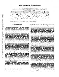
Thus, if s 51 only distributions with ^ l 2 & .1 are considered. The optimal solution in that case is close to the one obtained with a quadratic potential @8#. Quadratic potentials detect the direction extremizing the variance of the training set, which we call variance learning. We show below that the optimal overlap may be much larger than the one obtained through variance learning if the clusters have s ,1. Introducing the expression of V * obtained from Eqs. ~21! and ~2! into Eq. ~17! gives a as a function of R opt . It turns out that, for some values of a , this function has three different roots for R opt( a ), as is apparent in Figs. 1 and 2. The one lying on the branch with negative slope violates the assumption of replica symmetry. The two others correspond to minimas of the corresponding free energies. Figures 1, 2, and 3 show the optimal learning curves for several values of r and s in the range not investigated before. The two branches R opt( a ) with positive slope that satisfy condition ~16!, and the dotted line of negative slope ~inconsistent with the assumption of replica symmetry!, are presented for illustration. The value of a at which the jump from one branch to the other occurs is discussed in the next section. The performance obtained through learning with simple quadratic po-

3330

ARNAUD BUHOT AND MIRTA B. GORDON

FIG. 1. Learning curves for the two-cluster scenario, for cluster parameters corresponding to the lowest small square of Fig. 6. Full line, optimal learning; dash-dotted lines, lower branch of metastable solutions to optimal learning. Also shown is the replica-symmetry unstable curve ~dotted line!. The lowest dashed line corresponds to learning with a quadratic potential ~variance learning!. Here, a 1 53.79, R opt( a 1 )50.84; the Bayesian first order transition occurs at a G54.07, R opt( a G)50.9; the critical a for variance learning is a c 54.73.

57

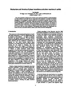
FIG. 3. Optimal learning curves ~full line! for the two-cluster scenario, for cluster parameters corresponding to the upper small square of Fig. 6. The lowest dashed line corresponds to learning with a quadratic potential ~variance learning!. Here, a c 50.68.

tentials is also presented, to show the dramatic improvement of optimal learning with respect to variance learning for double clusters with s ,1. V. BAYESIAN VERSUS OPTIMAL SOLUTIONS

FIG. 2. Learning curves for the two-cluster scenario, for cluster parameters corresponding to the central small square of Fig. 6. Full line, optimal learning; dash-dotted lines, lower branch of metastable solutions to optimal learning. Also shown is the replica-symmetry unstable curve ~dotted line!. The lowest dashed line corresponds to learning with a quadratic potential ~variance learning!. Here, a 1 52.49, R opt( a 1 )50.76; the Bayesian first order transition occurs at a G52.52, R opt( a G)50.81; the critical a for variance learning is a c 52.10.

As pointed out in Sec. III, Eq. ~17! may be deduced in two different ways: through the determination of the Bayesian learning performance, or through functional optimization. This procedure yields of a cost function for each training set size a whose minimum gives the solution with maximal overlap. The Bayesian solution to the learning problem is given by the average of solutions sampled with Gibbs’ probability. A simple argument @8# shows that the typical Bayesian performance satisfies R b5 AR G, where R G is the typical overlap between a solution drawn with probability ~5! and the symmetry-breaking direction B. R G minimizes the free energy with potential V( g )5V * ( g ) at inverse temperature b51 @8,7#. As Eq. ~17! is satisfied both by R b and R opt , it is tempting to conclude that Bayesian learning is optimal. If Eq. ~17! has a unique solution, this is obviously the case. However, Eq. ~17! may not be invertible. This arises in the two-cluster scenario presented in the preceding section, where two branches of solutions consistent with the assumption of replica symmetry exist for some values of a . In the case of Bayesian learning, these branches result from the fact that Gibbs’ free energy has two local minima as a function of R. R G , the thermodynamically stable state, corresponds to the absolute minimum. When a changes, R G jumps from one branch to the other through a first order phase transition at a 5 a G , where both minima have the same free energy @12#. Therefore the Bayesian solution, which is the average of the solutions sampled with Gibbs’ probability, presents a jump at the same value a G as Gibbs’ performance. Thus, the meta-

57

PHASE TRANSITIONS IN OPTIMAL UNSUPERVISED . . .

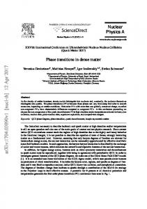
FIG. 4. Learning curves for r 51.1, s 50.5 obtained with the optimal potentials corresponding to R opt50.84, R opt50.87, and R opt50.90 ~full lines!. Only the solutions consistent with the replica-symmetry hypothesis are shown. Dotted lines: optimal solution.

stable states of higher performance than R b , which exist for a , a G , cannot be obtained through Bayesian learning. On the other hand, in Sec. III we determined optimal potentials whose minimization allows to obtain performance R opt . These potentials exist for all the pairs „a ,R opt( a )… lying on the monotonically increasing branches of R opt( a ), which satisfy the hypothesis of replica symmetry. Potentials allowing to reach the performances of the upper ~Gibbsmetastable! branch thus exist. It should be noticed that we cannot determine the position of the jump of R opt through the comparison of the free energies corresponding to solutions on different branches at the same a , as was done to determine a G , because a different potential has to be minimized for each pair „a ,R opt( a )… and, as discussed in Sec. III, these potentials are measured in the arbitrary units determined by our choice c51. In order to clarify this problem, we studied the performance of the minima of the optimal potentials. In fact, the properties of each of the potentials V opt(l) may be determined for any value of a ~besides the value for which it has been optimized! in the same way as those of other ad hoc potentials, by solving numerically Eq. ~14!. Figures 4 and 5 present several learning curves R( a ) obtained with potentials V opt optimized for overlaps lying on the upper metastable branch of Gibbs’ learning. They correspond to the same clusters’ parameters as Figs. 1 and 2. Each learning curve is tangent to the optimal learning curve at the point „a (R opt),R opt… at which the potential was determined. This result holds in particular for all the points lying on the highperformance metastable branch of Bayesian learning, i.e., for a 1 , a , a G . It is important to point out that the free energy ~11! presents a unique replica-symmetric minimum as a function of R for all these potentials. Thus, these results show that the corresponding optimal potentials V opt allow to select, among the metastable states of Gibbs learning, the one of largest overlap. In particular, the Gibbs’ metastable states in the upper branch for a , a G are learnable through the minimization of the corresponding optimal potential.

3331

FIG. 5. Learning curves for r 51.2, s 50.5 obtained with the optimal potentials corresponding to R opt50.76, R opt50.79 and R opt50.81 ~full lines!. Only the solutions consistent with the replica- symmetry hypothesis are shown. Dotted lines: optimal solution.

Thus, in the range a 1 , a , a G , Bayesian learning is not optimal. This surprising behavior may arise whenever the curve R G( a ) of Gibbs learning presents first order phase transitions. It is worth noting that, besides the solutions that verify the replica-symmetric condition ~16!, solutions unstable under replica-symmetry breaking with smaller R and slightly higher free energy also exist. The nature of these states is very different from that of the metastable states of Gibbs learning. Whether the typical performance in the case of the double cluster distributions is the one described by the replica-symmetric solution or not remains an open problem. VI. THE PHASE DIAGRAM

In this section we describe, on the r -s plane, all the possible learning phases that may arise in unsupervised learning within the two-Gaussian-cluster scenario. As shown in Fig. 6, depending on the values of r and s , qualitatively different behaviors of the learning curves R opt( a ) may appear. They are correlated with the form of the corresponding optimal potentials. The regions marked with an ‘‘S’’ are regions of variancetype learning: the optimal potential is a single well with V opt→1` for l→6` if s 2 ,1, and V opt→2` for l→ 6` if s 2 .1. In these regions, the learning curves increase monotonically with a , starting at a c 5 u ^ l 2 & 21 u 22 , as for quadratic potentials @4#. For parameter values outside the ‘‘S’’ regions, V opt→ 1` for l→6`, even in the large variance region ^ l 2 & .1 where naively one would expect the potential to have the same asymptotic behavior as for s 2 .1. Depending on the value of R opt , the optimal potential may be a double-well function of the local field g . In the latter case, the optimal learning strategy looks for structure in the data distribution rather than for directions extremizing the variance. This is more striking on the line ^ l 2 & 51 corresponding to distribu-

3332

ARNAUD BUHOT AND MIRTA B. GORDON

57

FIG. 7. Potentials for optimal learning in the grey regions of the phase diagram, showing the evolution of the separation between minima with a . VII. CONCLUSION

FIG. 6. Phase diagram of the two-cluster scenario. The three small squares correspond to the learning curves of Figs. 1, 2, and 3.

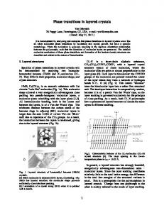
tions with the same second moment in all the directions. On this line, variance learning is impossible and a c 5`. However, in the entire light-gray region including this line, performant learning is achieved if the adequate potential is minimized. The optimal overlap presents jumps from R opt 50 to finite R at a fraction of examples a , a c . In the highperformance branch, the optimal potential is double-well, with the two minima close to 6 r , as shown in Fig. 7. Thus, the potential is sensitive to the two-cluster structure, and its minimization results in high performance learning. For r and s in the dark-gray regions, a first order transition to large R also takes place, but for a . a c . Below the transition, optimal learning is mainly controlled by the variance of the training set. In the white regions on both sides of the dark-gray ones, no first order phase transitions to high performance learning occur as a function of a . In the white region just below the dark-gray one, the potential changes smoothly from a single to a double well with increasing R opt . The two minimas appear at g 50, and move away with increasing R opt , as shown in Fig. 8. However, as far as these minimas are not sufficiently apart, R opt remains close to the values obtained with simple quadratic potentials. Conversely, in the upper white region, which corresponds to ^ l 2 & @1, the minima of the optimal potential are far apart, in a region of large local fields, where the patterns’ distribution is vanishingly small. Thus, in the range of pertinent values of g the potential is concave (V 9opt,0), and here also, as in the lower white region, the values of R opt are close to those obtained with quadratic potentials @4#.

Learning the symmetry-breaking direction of a distribution of patterns with axial symmetry in high dimensions is a difficult problem. In this paper we determined the optimal performances that may be reached if the patterns distribution has a double-cluster structure in the symmetry-breaking direction. Depending on the clusters’ size and separation, the learning curves may present several phases with increasing a , including novel first order transitions from lowperformance variance learning to high-performance structure

FIG. 8. Potentials for optimal learning in the white regions of the phase diagram, showing the appearance of the two minima that get farther apart with increasing a .

57

PHASE TRANSITIONS IN OPTIMAL UNSUPERVISED . . .

detection. We showed that when the optimal learning curves present such discontinuities, Bayesian learning may be not optimal. These results rely on the assumption that the solution with replica symmetry is the absolute minimum of the free energies studied. Although we showed that our solutions satisfy the replica symmetry stability condition, we cannot

@1# R. O. Duda and P. E. Hart, Pattern Classification and Scene Analysis ~John Wiley and Sons, New York, 1973!. @2# B. Ripley, Pattern Recognition and Neural Networks ~Cambridge University Press, Cambridge, 1996!. @3# T. Kohonen, Self-Organizing Maps ~Springer, Berlin, 1995!. @4# P. Reimann and C. Van den Broeck, Phys. Rev. E 53, 3989 ~1996!. @5# O. Kinouchi and N. Caticha, Phys. Rev. E 54, R54 ~1996!. @6# A. Buhot, J. M. Torres Moreno, and M. B. Gordon, Phys. Rev. E 55, 7434 ~1997!.

3333

rule out the existence of states of lower energy, but having broken replica symmetry. ACKNOWLEDGMENTS

We thank Chris Van den Broeck and Mauro Copelli for helpful discussions at the early stages of this work.

@7# C. Van den Broeck and P. Reimann, Phys. Rev. Lett. 76, 2188 ~1996!. @8# T. L. H. Watkin and J.-P. Nadal, J. Phys. A 27, 1899 ~1994!. @9# P. Reimann, C. Van den Broeck, and G. J. Bex, J. Phys. A 29, 3521 ~1996!. @10# M. Biehl and A. Mietzner, Europhys. Lett. 24, 421 ~1993!. @11# M. Biehl and A. Mietzner, J. Phys. A 27, 1885 ~1994!. @12# M. Copelli ~private communication!.