work on dataflow graphs and SARE's (Section 2). ..... 2. There are no initialization phases: ân, num(n, init) = 0. 3. Each node has only one steady-state phase: ...
Phased Computation Graphs in the Polyhedral Model
∗
William Thies, Jasper Lin and Saman Amarasinghe MIT Laboratory for Computer Science Cambridge, MA 02139 {thies, jasperln, saman}@lcs.mit.edu
Abstract We present a translation scheme that allows a broad class of dataflow graphs to be considered under the optimization framework of the polyhedral model. The input to our analysis is a Phased Computation Graph, which we define as a generalization of the most widely used dataflow representations, including synchronous dataflow, cyclo-static dataflow, and computation graphs. The output of our analysis is a System of Affine Recurrence Equations (SARE) that exactly captures the data dependences between the nodes of the original graph. Using the SARE representation, one can apply many techniques from the scientific community that are new to the DSP domain. For example, we propose simple optimizations such as node splitting, decimation propagation, and steady-state invariant code motion that leverage the fine-grained dependence information of the SARE to perform novel transformations on a stream graph. We also propose ways in which the polyhedral model can offer new approaches to classic problems of the DSP community, such as minimizing buffer size, code size, and optimizing the schedule.
1
Introduction
Synchronous dataflow graphs have become a powerful and widespread programming abstraction for DSP environments. Originally proposed by Lee and Messerchmitt in 1987 [18], synchronous dataflow has since evolved into a number of varieties [5, 1, 26, 6] which provide a natural framework for developing modular processing blocks and composing them into a concurrent network. A dataflow graph consists of a set of nodes with channels running between them; data values are passed as streams over the channels. The synchronous assumption is that a node will not fire until all of its inputs are ready. Also, the input/output rates of the nodes are known at compile time, such that a static schedule can be computed for the steadystate execution. Synchronous dataflow graphs have been shown to successfully model a large class of DSP applications, including speech coding, auto-correlation, voice band modulation, and a number of filters. A significant industry has emerged to provide dataflow design environments; leading products include COSSAP from Synopsys, SPW from Cadence, ADS from Hewlett Packard, and DSP Station from Mentor Graphics. Academic projects include prototyping environments such as Ptolemy [17] and Grape-II [16] as well as languages such as Lustre [13], Signal [10], and StreamIt [11]. ∗ This
document is MIT Laboratory for Computer Science Technical Memo LCS-TM-???, August 2002. Our latest work on this subject will be available from http://cag.lcs.mit.edu/streamit
1
Optimization is especially important for signal processing applications, as embedded processors often have tight resource constraints on speed, memory, and power. In the synchronous dataflow domain, this has resulted in a number of aggressive optimizations that are specially designed to operate on dataflow graphs–e.g., minimizing buffer size while restricting code size [25], minimizing buffer size while maintaining parallelism [12], resynchronization [4], and buffer sharing [24]. While these optimizations are beneficial, they unilaterally regard each node as a black box that is invisible to the compiler. Blocks are programmed at a coarse level of granularity, often with hand-tweaked implementations inside, and optimizations are considered only when stitching the blocks together. In some sense at the other end of the spectrum are the optimization techniques of the scientific computing community. These are characterized by fine-grained analyses of loops, statements, and control flow, starting from sequential C or FORTRAN source code that lacks the explicit parallelism and communication of a dataflow graph. Out of this community has come a number of general methods for precise, fine-grained program analysis and optimization. In the context of array dataflow analysis and automatic parallelization, one such framework is the polyhedral model [7], which represents programs as sets of affine relations over polyhedral domains. In recent years, it has been shown that affine dependences can exactly represent the flow of data in certain classes of programs [8], and that affine partitioning can subsume loop fusion, reversal, permutation, and reindexing as a scheduling technique [21]. Moreover, affine scheduling can operate on a parameterized version of the input program, avoiding the need to expand a graph for varying parameters and problem sizes, and it can often reduce to a linear program for flexible and efficient optimization. Polyhedral representations have also been utilized for powerful storage optimizations [22, 28, 31, 20]. In this paper, we aim to bridge the gap and employ the polyhedral representations of the scientific community to analyze the synchronous dataflow graphs of the DSP community. Towards this end, we present a translation from a dataflow graph to a System of Affine Recurrence Equations (SARE), which are equivalent to a certain class of imperative programs and can be used as input to the affine analysis described above. The input of our analysis is a “Phased Computation Graph” (PCG), which we formalize as a generalization of several existing dataflow frameworks. Once a PCG is represented as a SARE, we demonstrate how affine techniques could be employed to perform novel optimizations such as node splitting, decimation propagation, and steady-state invariant code motion that exploit both the structure of the dataflow graph as well as the internal contents of each node. We also discuss the potential of affine techniques for scheduling parameterized dataflow graphs, as well as offering new approaches to classic problems in the dataflow domain. The rest of this paper is organized as follows. We begin by describing background information and related work on dataflow graphs and SARE’s (Section 2). Then we define a Phased Computation Graph (Section 3) and Phased Computation Program (Section 4), and give the procedure for translating a simple, restricted PCP to a SARE (Section 5). Next, we give the full details for the general translation (Section 6), describe a range of applications for the technique (Section 7), and conclude (Section 8). A detailed example that illustrates our technique appears in the Appendix.
2 2.1
Background and Related Work Dataflow Graphs
Strictly speaking, synchronous dataflow (SDF) refers to a class of dataflow graphs where the input rate and output rate of each node is constant from one invocation to the next [18, 19]. For SDF graphs, it is straightforward to determine a legal steady state schedule using balance equations [3] (see Section 5.1). The SDF scheduling community focuses on “single-appearance schedules” (SAS) in which each filter appears at 2
only one position in the loop nest denoting the schedule. The interest in SAS is because the runtime overhead of a method call is prohibitive, so the code for each block is inlined. However, code size is so important that they can’t afford to duplicate the inlining, thus leading to the restriction that each filter appear only once. They have demonstrated that minimizing buffer size in general graphs is NP-complete, but they explore two heuristics to do it in acyclic graphs [2]. Cyclo-static dataflow (CSDF) is the generalization of SDF to the case where each node has a set of phases with different I/O rates that are cycled through repeatedly [5, 27]. Compared to SDF, CSDF is more natural for the programmer for writing phased filters, since periodic tasks can be separated. For instance, consider a channel decoder that inputs a large matrix of coefficients at regular intervals, but decodes one element at a time for N invocations in between each set of coefficients. By having two separate phases, the programmer doesn’t have to interleave this functionality in a single, convoluted work function. Also, CSDF can have lower latency and more fine-grained parallelism than SDF. However, current scheduling techniques for CSDF involve converting each phase to an SDF actor, which can cause deadlock even for legal graphs [5] and does not take advantage of the fine-grained dataflow exposed by CSDF. The computation graph (CG) was described by Karp and Miller [15] as a model of computation that, unlike the two above, allows the nodes to peek. By “peek” we mean that a node can read and use a value from a channel without consuming (popping) it from the channel; peeking is good for the programmer because it automates the buffer management for input items that are used on multiple firings, as in an FIR filter. However, peeking complicates the schedule because an initialization schedule is needed to ensure that enough items are on the channel in order to fire [11]. In [15], conditions are given for when a computation graph terminates and when its data queues are bounded. Govindarajan et. al develop a linear programming framework for determining the “rate-optimal schedule” with the minimal memory requirement [12]. A rate-optimal schedule is one that takes advantage of parallel resources to execute the graph with the maximal throughput. Though their formulation is attractive and bears some likeness to ours, it is specific for rate-optimal schedules and does not directly relate to the polyhedral model. It also can result in a code size blow up, as the same node could be executed in many different contexts.
2.2
Systems of Affine Recurrence Equations
A System of Affine Recurrence Equations (SARE) is a set of equations E1 . . . EmE of the following form [7, 8]: ∀~i ∈ DE : X(~i) = fE (. . . , Y (~hE,Y (~i)), . . . )
(1)
In this equation, our notation is as follows: • {X, Y, . . . } is the set of variables defined by the SARE. Variables can be considered as multi-dimensional arrays mapping a vector of indices ~i to a value in some space V. • DE is a polyhedron representing the domain of the equation E. Each equation for a variable X has a disjoint domain; the domain DX for variable X is taken as the convex union of all domains over which X is defined. • ~hE,Y is a vector-valued affine function, giving the index of variable Y that X(~i) depends on. A vector~ where C is a constant array and d~ is a valued function ~h is affine if it can be written as ~h(~i) = C~i + d, constant vector that do not vary with ~i. • fE is a strict function used to compute the elements of X. 3
Model of Computation Synchronous Dataflow [18] Cyclo-Static Dataflow [5] Computation Graphs [14] Phased Computation Graphs
Items on Channels at Start X X X X
Nodes with Pop 6= Push X X X X
Nodes with Peek > Pop
Cyclic Steady State Phases
Initialization Phases
X X X
X
X
Table 1: Models of Computation for Dataflow Graphs. Intuitively, the SARE can be considered as follows. Given an array element at a known index ~i, the SARE gives the set of arrays and indices that this element depends on. Furthermore, each index expression on the right hand side is an affine expression of ~i. Note that in order to map directly from an array element to the elements that it depends on, the index expression on the left hand side must exactly match the domain quantifier ~i. A SARE has no notion of internal state per se; however, state can be modeled by introducing a self-loop in the graph of variables. If the dependence function ~h happens to be a translation (~h(~i) = ~i − ~k for constant ~k), then the SARE is uniform, and referred to as a SURE or SRE [15]. SURE’s can be used for systolic array synthesis [29], and there are techniques to uniformize SARE’s into SURE’s [23]. SARE’s became interesting from the standpoint of program analysis upon Feautrier’s discovery [8, 9] that a SARE is mathematically equivalent to a “static control flow program”. A program has static control flow if the entire path of control can be determined at compile time (see [8, 7] for details). Feautrier showed that using a SARE, one can use linear programming to produce a parameterized schedule for a program. That is, if a loop bound is unknown at compile time, then the symbolic bound enters the schedule and it does not affect the complexity of the technique. Feautrier’s framework is very flexible in that it allows one to select a desirable affine schedule by any linear heuristic. Lim and Lam [22] build on Feautrier’s technique with an affine partitioning algorithm that maximizes the degree of parallelism while minimizing the degree of synchronization. It also operates on a form that is equivalent to a SARE.
3
Phased Computation Graphs
We introduce the Phased Computation Graph (PCG) as a model of computation for dataflow languages; specifically, we designed the PCG as a model for StreamIt [30]. A PCG is a generalization of the Computation Graph (CG) of Karp and Miller [14] to the case where each node has both an initial and steady-state execution epoch, each of which contains a number of phases. It is also a generalization of other popular representations for dataflow graphs, such as synchronous dataflow (SDF) and cyclo-static dataflow (CSDF) (see Table 1). Phases are attractive constructs for the reasons given in describing CSDF in Section 2; also, an initial epoch is critical for applications such as a WAV file decoder that adjusts its parameters based on the data it finds in the header of the stream. Formally, a PCG is a directed graph with the following components: • Nodes n1 . . . nmn . • Channels c1 . . . cmc , where each channel is directed from a given node na to a given node nb . • A non-negative integer A(c) indicating the number of items that are initially present on channel c.
4
• The number of phases num(n, t) that node n exhibits during epoch t. Here t indicates the type of epoch, which is either initial (init) or steady-state (steady). For all n, num(n, init) ≥ 0 and num(n, steady) ≥ 1. • Non-negative integers U (c, t, p), O(c, t, p), and E(c, t, p), which give the number of items pushed, popped, and peeked, respectively, over channel c during the p’th phase of epoch t.
3.1
Execution Model
We give an informal description of the execution semantics of a PCG, which is an intuitive extension to that of a CG. An execution consists of a sequence of atomic firings of nodes in the graph. The effect of firing a given node depends on its epoch and its phase, which are both local states of the node. At the start of execution, each node is in phase 0 of the initial epoch, and each channel c contains A(c) items. Let us consider a node n that is in phase p of epoch t. It is legal for n to fire if p ∈ [0, num(n, t) − 1] and, for each channel cin directed into n, there are at least E(cin , t, p) items on cin . The effect of this firing is to consume O(cin , t, p) items from each channel cin directed into n; to produce U (cout , t, p) new items on each channel cout directed out of n; and to advance the phase p of n to next(t, p). In the initial epoch, each phase executes only once and next(init, p) = p + 1; in the steady-state epoch, the phases execute cyclically and next(steady, p) = (p + 1) mod num(n, t). If a node n is in phase num(n, init) of the initial epoch, then it transitions to the steady-state epoch and resets its phase to 0. From the starting state of the graph, execution proceeds via an infinite sequence of node firings. The order of node firings is constrained only by the conditions given above.
4
Phased Computation Programs
The PCG described above is a representation for a graph, treating each node and channel as a black box. Here we introduce some notation for the internals of the nodes, as well as the ordering of items on the channels. We refer to the aggregate model as a Phased Computation Program (PCP). Before describing a PCP, we will need some additional notation: • We assume that all items passed over channels are drawn from the same domain of values V. • An array type1 of length n and element type τ is denoted by τ [n]. Given a two-dimensional array A of type τ [n][m], A[i][∗] denotes the m-element array comprising the i’th row of A. • num in(n) (resp. num out(n)) denotes the number of channels that are directed into (resp. out of) node n. • chan in(n) (resp. chan out(n)) denotes the list of channels that are directed into (resp. out of) node n. • pos in(n, c) (resp. pos out(n, c)) denotes the position of channel c in chan in(n) (resp. chan out(n). That is, chan out(n)[pos out(n, c)] = c.
1 To simplify the presentation, we allow ourselves a slight abuse of notation by sometimes using arrays instead of enumerating individual elements. Our definitions could be expanded into strict element-wise SARE’s without any fundamental change to the technique.
5
A PCP consists of the following: • A Phased Computation Graph G = ({n1 . . . nmn }, {c1 . . . cmc }, A, num, U, O, E) describing the nodes, channels, and I/O rates of the program (see Section 3). Each channel c = (n a , nb ) is a FIFO queue; na pushes items onto the back of c and nb consumes items from the front of c. • The initial values I(c) that are enqueued onto channel c at the start of execution. Since there are A(c) initial values on channel c, I(c) has type V[A(c)]. • A work function W (n, t, p) that represents the computation of node n in phase p and epoch t. The signature of W (n, t, p) is [V[E(chan in(n)[1], t, p)], . . . , V[E(chan in(n)[num in(n)], t, p)]] → [V[U (chan out(n)[1], t, p)], . . . , V[U (chan out(n)[num out(n)], t, p)]]. That is, the function inputs a list of arrays, each of which corresponds to an incoming channel cin and contains the E(cin , t, p) values that n reads from cin in a given firing. The procedure returns a list of arrays, each of which corresponds to an outgoing channel cout and contains the U (cout , t, p) values that n writes to cout in a given firing.
5
Basic Translation: CG to SARE
In order to familiarize the reader with the basics of our technique, we present in this section the translation procedure for a simplified input domain. The translation rules for the general case can be found in Section 6. Our basic translation operates on computation graphs with all of the channels initially empty. That is, we assume that: 1. No items appear on the channels at the beginning: ∀c, A(c) = 0. 2. There are no initialization phases: ∀n, num(n, init) = 0. 3. Each node has only one steady-state phase: ∀n, num(n, steady) = 1. Given these restrictions, we can simplify our notation considerably. Since we are only concerned with the steady-state epoch and the 0’th phase of each node, we can omit some arguments to any function that requires an epoch t or a phase p. For instance, the push and pop rates of a channel c are now just U (c) and O(c), respectively; the work function for a node n is simply W (n).
5.1
Calculating the Steady-State Period
Let S(n) denote the number of times that node n fires its first phase for a periodic steady-state execution of the entire graph. A periodic schedule is one that does not change the number of items on the channels in the graph after executing; in other words, it is legal to execute in the steady state. For an SDF graph, there is a unique and minimal periodic schedule, of which all other periodic schedules are a multiple [3]. It is straightforward to use a set of balance equations to solve for S(n) given the declared rates of filters in the graph. If the graph is invalid (i.e., it would lead to deadlock or an unbounded buffer size) then the balance equations will have no solution. See [3] for details. We will use the following helper function in our analysis. Given channel c = (n a , nb ): Period(c) ≡ S(na ) ∗ U (c) = S(nb ) ∗ O(c) That is, Period(c) denotes the number of items that are passed over channel c during a single steady-state execution of the graph. 6
Variables For each channel c = (na , nb ), do the following: • Introduce variable BUFc with the following domain: DBU F c = { (i, j) | 0 ≤ i ≤ N − 1 ∧ 0 ≤ j ≤ Period(c) − 1}
(2)
• Introduce variable WRITEc with this domain: DW RIT E c = { (i, j, k) | 0 ≤ i ≤ N − 1 ∧ 0 ≤ j ≤ S(na ) − 1 ∧ 0 ≤ k ≤ U (c) − 1}
(3)
• Introduce variable READc with this domain: DREADc = { (i, j, k) | 0 ≤ i ≤ N − 1 ∧ 0 ≤ j ≤ S(nb ) − 1 ∧ 0 ≤ k ≤ E(c) − 1}
(4)
Equations For each node n, introduce the following equations: • (READ to WRITE) For each c ∈ chan out(n): ∀(i, j, k) ∈ DW RIT E c : WRITEc (i, j, k) = W (n)(Steady Inputs)[pos out(n, c)][k]
(5)
where Steady Inputs = [READchan in(n)[0] (i, j, ∗), . . . , READchan in(n)[num in(n)−1] (i, j, ∗)] • (WRITE to BUF) For each c ∈ chan out(n), and for each q ∈ [0, S(n) − 1]: ∀(i, j) ∈ DW →B (c, q) : BUFc (i, j) = WRITEc (i, q, j − q ∗ U (c))
(6)
where DW →B (c, q) = DBU F c ∩ {(i, j) | q ∗ U (c) ≤ j ≤ (q + 1) ∗ U (c) − 1} • (BUF to READ) For each c ∈ chan in(n), and for each q ∈ [0, b
E(c)
Period(c)
c]:
∀(i, j, k) ∈ DB→R : READc (i, j, k) = BUFc (i + q, j ∗ O(n) + k − q ∗ Period(c))
(7)
where DB→R = DREADc ∩ {(i, j, k) | q ∗ Period(c) ≤ k ≤ min((q + 1) ∗ Period(c), E(c)) − 1} Figure 1: Procedure for generating a SARE from a simplifed PCP: one that has only one epoch, one phase, and no initial tokens.
7
5.2
Generating a SARE
We now generate a SARE for the simplified instance of a PCP. The domains of the SARE will be parameterized by N , the number of steady-state cycles that one wishes to execute in the PCP. However, it is important to note that N does not affect the number of variables or equations in the SARE, as that would require a separate compilation and analysis for each value of N . It is a key benefit of the SARE representation that N can be incorporated as a symbolic parameter in the schedule. The procedure for generating the SARE appears in Figure 1. The basic idea is to introduce a variable BUFc for each channel c which keeps track of the entire history of values that are transmitted over c (we keep track of the entire history since all elements in a SARE must be assigned only once.) The i dimension of BUF counts over steady-state periods, while the j dimension holds elements that were written during a given period. We also introduce variables WRITEc and READc that write and read from channel c. For reasons that become clear below, these variables have a k dimension to index the values that are pushed on a given firing, while the j dimension counts firings of a node and the i dimension counts steady-state periods, as before. Equation 5 expresses the computation internal to each node, whereas Equations 6 and 7 expresses the communication of the nodes with the channels. In Equation 5, the node’s work function is used to calculate all of the WRITE values from all of the READ values, during a given firing (i, j). Equation 6 shows the communication from the WRITE array to the BUF array for a given channel. To understand this equation, it might help to consider a simpler version which expresses the correct relationship but is not a legal SARE: ∀(i, j, k) ∈ DWRITEc : BUFc (i, j ∗ U (c) + k) = WRITEc (i, j, k) The equation above is simply copying the contents of WRITE into BUF while accounting for the differing array dimensions. However, this equation is not valid for a SARE, since there is an affine expression indexing the array on the left hand side. To deal with this issue, we split up the equation into several pieces, each of which assigns to a different portion of the BUF array. In Equation 6, we introduce a variable q that counts up to S(n), which is the extent of the j dimension of WRITEc . For each of these q, we copy over U (c) values from the appropriate section of the WRITE array; the domain DW →B (c, q) represents the q’th slice of BUF into which the section should be written. This equation is a valid component of our SARE, as the boundaries on each equation’s domain are fully resolvable at compile time. Equation 7 is similar to Equation 6 regarding the slicing technique that is used to parameterize the domain of the equation. However, here the motivation is different: the extent of the k dimension of READ might exceed the length of the period in BUF (this is because nodes are allowed to peek more than they pop.) Thus, the q variable is used to slice the peek amount E(c) into Period(c)-sized chunks so as to resolve the proper source location in BUF. Again, all the variables in the index expressions are compile-time constants (except, of course, for the index quantifiers i, j, and k.)
6
General Translation: PCP to SARE
In this section we give the formal translation of a Phased Computation Program to a System of Affine Recurrence Equations. Again, the SARE will be parameterized by N , the number of steady-state cycles that one wishes to execute in the PCP. The translation will use the helper functions shown in Figure 2. We
8
Helper Functions • The number of integral points in a one-dimensional domain D is denoted by |D|. The sign and absolute value of an integer i are given by sign(i) and abs(i), respectively. Pp−1 • PartialWrite(c, t, p) = r=0 U (c, t, r) Pnum(n,t)−1 • TotalWrite(n, c, t) = r=0 U (c, t, r) Pp−1 • PartialRead(c, t, p) = r=0 O(c, t, r) Pnum(n,t)−1 • TotalRead(n, c, t) = r=0 O(c, t, r) • Given channel c = (na , nb ): Period(c) ≡ S(na ) ∗ TotalWrite(na , c, steady) = S(nb ) ∗ TotalRead(nb , c, steady) Figure 2: Helper functions for the PCP to SARE translation. also make use of the S(n) function giving the number of steady-state executions of node n (see Section 5.1). Please refer to the Appendix for a concrete illustration of the techniques described below. Figure 3 illustrates the variables used for the translation. These are very similar to those in the simple case, except that now there are separate variables for initialization and steady state, as well as variables for each phase. The equations for the translation appear in Figures 5 and 6. A diagram of which variables depend on others appears in Figure 4. Due to space limitations, we discuss only the most interesting parts of the translation below. Equation 14 writes the initial values of the initial tokens on IBUF, the initial buffer. Equation 15 transfers values from the initial epoch of a node to the initial buffer of a channel. Equations 16 and 17 do the work computation of the initial and steady-state items, respectively, just as in the simple translation of Section 5.2. Equation 18 copies items from the node to the channel, using the same slicing technique as Equation 6. Equation 19 copies values from the initial buffer (IBUF) of a channel into the initial read array for a node. However, since the node might read more items in the initial epoch than exist on the initial buffer, we restrict the domain of the equation to only those indices that have a corresponding value in IBUF. If it is the case that there are fewer items in the initial buffer than a node reads in its initial epoch, then Equation 20 copies values from the beginning of the channel’s steady-state buffer into the remaining locations on the node’s initial array. The upper bound for q in Equation 20 is calculating the maximum amount that any phase peeks in the initialization epoch, so that enough equations are defined to fill the node’s initial read array. Note that for some phases, the dependence domain of Equation 20 will be empty, in which case no equation is introduced. Also, Equation 20 uses the slicing method (see Section 5.2) because the initial read array is of lower dimensionality than the steady-state buffer from which it is reading. Equation 21 is dealing with the opposite case as Equation 20: when a node finds items on its channel’s initial buffer when it is entering the steady-state epoch. In this case copying over the appropriate items to the beginning of the steady-state read array is rather straightforward. Much of the complexity of the entire translation is pushed into Equations 22 and 23. There are two distinct complications in these equations. First is one that we tackled in Equation 7: the fact that the read array might peek beyond the limits of the buffer, which requires us to slice the domain in increments of one period. The second complication is that there could be an offset–an initial buffer might have written into
9
Variables For each channel c = (na , nb ), do the following: • Introduce variables IBUFc and SBUFc with the following domains: num(na ,init)−1
X
U (c, init, p)}
(8)
DSBU F c = { (i, j) | 0 ≤ i ≤ N − 1 ∧ 0 ≤ j ≤ Period(c) − 1}
(9)
DIBU F c = { i | 0 ≤ i ≤ A(c) − 1 +
p=0
• For each p ∈ [0, num(na , init) − 1], introduce variable IWRITEc,p with this domain: DIW RIT E c,p = { i | 0 ≤ i ≤ U (c, init, p) − 1}
(10)
• For each p ∈ [0, num(nb , init) − 1], introduce variable IREADc,p with this domain: DIREADc,p = { i | 0 ≤ i ≤ E(c, init, p) − 1}
(11)
• For each p ∈ [0, num(na , steady) − 1], introduce variable SWRITEc,p with this domain: DSW RIT E c,p = { (i, j, k) | 0 ≤ i ≤ N − 1 ∧ 0 ≤ j ≤ S(na ) − 1 ∧ 0 ≤ k ≤ U (c, steady, p) − 1} (12) • For each p ∈ [0, num(nb , steady) − 1], introduce variable SREADc,p with this domain: DSREADc,p = { (i, j, k) | 0 ≤ i ≤ N − 1 ∧ 0 ≤ j ≤ S(nb ) − 1 ∧ 0 ≤ k ≤ E(c, steady, p) − 1} (13) Figure 3: Variables for the PCP to SARE translation.
I
IBUF
SREAD
SWRITE
SBUF
IWRITE
IREAD
Figure 4: Flow of data between SARE variables. Data flows from the base of each arrow to the tip. Dotted lines indicate communication that might not occur for a given channel.
10
Equations (Part 1 of 2) For each channel c = (na , nb ), introduce the following equations: • (I to IBUF):
∀i ∈ [0, A(c) − 1] : IBUFc (i) = I(c)[i]
(14)
• (IWRITE to IBUF) For each p ∈ [0, num(na , init) − 1]: ∀i ∈ [A(c) + PartialWrite(c, init, p), A(c) + PartialWrite(c, init, p + 1) − 1] :
(15)
IBUFc (i) = IWRITEc,p (i − A(c) − PartialWrite(c, init, p)) For each node n, introduce the following equations: • (IREAD to IWRITE) For each c ∈ chan out(n), and for each p ∈ [0, num(n, init) − 1]: ∀i ∈ DIW RIT E c,p : IWRITEc,p (i) = W (n, init, p)(Init Inputs)[pos out(n, c)][i],
(16)
where Init Inputs = [IREADchan in(n)[0],p (∗), . . . , IREADchan in(n)[num in(n)−1],p (∗)] • (SREAD to SWRITE) For each c ∈ chan out(n), and for each p ∈ [0, num(n, steady) − 1]: ∀(i, j, k) ∈ DSW RIT E c,p : SWRITEc,p (i, j, k) = W (n, steady, p)(Steady Inputs)[pos out(n, c)][k], where
(17)
Steady Inputs = [SREADchan in(n)[0],p (i, j, ∗), . . . , SREADchan in(n)[num in(n)−1],p (i, j, ∗)] • (SWRITE to SBUF) For each c ∈ chan out(n), for each p ∈ [0, num(n, steady) − 1], and for each q ∈ [0, S(n) − 1]: ∀(i, j) ∈ DSW →SB (c, p, q) : SBUFc (i, j) = SWRITEc,p (i, q, j − OffsetSW →SB (q, n, c, p)), where
(18)
DSW →SB (c, p, q) = DSBU F c ∩ {(i, j) | OffsetSW →SB (q, n, c, p) ≤ j ≤ OffsetSW →SB (q, n, c, p + 1) − 1} and OffsetSW →SB (q, n, c, p0 ) = q ∗ TotalWrite(n, c, steady) + PartialWrite(c, steady, p0 )) • (IBUF to IREAD) For each c ∈ chan in(n), and for each phase p ∈ [0, num(n, init) − 1]: ∀i ∈ DIB→IR (c, p) : IREADc,p (i) = IBUFc (PartialRead(c, init, p) + i)
(19)
where DIB→IR (c, p) = {i | i ∈ DIREADc,p ∧ i + PartialRead(c, init, p) ∈ DIBU F c } • (SBUF to IREAD) For each c ∈ chan in(n), for each phase p ∈ [0, num(n, init) − 1], and for each argmaxp0 (PartialRead(c,init,p0 )+E(c,init,p0 )) q ∈ [0, b c]: Period(c) ∀i ∈ DSB→IR (c, p) : IREADc,p (i) = SBUFc (q, i − OffsetSB→IR (q, n, c, p)), where
(20)
DSB→IR (c, p) = {i | i ∈ DIREADc,p ∧ OffsetSB→IR (q, n, c, p) ≤ i ≤ OffsetSB→IR (q + 1, n, c, p) − 1} and OffsetSB→IR (q 0 , n, c, p) = q 0 ∗ Period(c) + |DIBU F c | − PartialRead(c, init, p) Figure 5: Equations for the PCP to SARE translation.
11
Equations (Part 2 of 2) For each node n, introduce the following equations: • (IBUF to SREAD) For each c ∈ chan in(n), and for each phase p ∈ [0, num(n, steady) − 1]: ∀(i, j, k) ∈ DIB→SR (n, c, p) : SREADc,p (i, j, k) = IBUFc (ReadIndex(n, c, p, i, j, k)), where ReadIndex(n, c, p, i, j, k) = TotalRead(n, c, init) + (i ∗ S(n) + j) ∗ TotalRead(n, c, steady)
(21)
+ PartialRead(c, steady, p) + k) and DIB→SR (n, c, p) = {(i, j, k) | ReadIndex(n, c, p, i, j, k) ∈ DIBU F c } • (SBUF to SREAD) For each c ∈ chan in(n), for each phase p ∈ [0, num(n, steady) − 1], and for E(c, steady, p) each q ∈ [0, b c]: Period(c) ∀(i, j, k) ∈ D1SB→SR (c, p, q) : SREADc,p (i, j, k) = SBUFc (i + q + Int Offset(n, c, p), j ∗ TotalRead(n, c, steady) + PartialRead(c, steady, p) + k − q ∗ Period(c) + Mod Offset(n, c, p)), where D1SB→SR (c, p, q) = (DSREADc,p − PUSHED(n, c, p)) ∩
(22)
{(i, j, k) | q ∗ Period(c) − min(0, Mod Offset(n, c, p)) ≤ k ≤ min((q + 1) ∗ Period(c), E(c, steady, p)) − 1 − max(0, Mod Offset(n, c, p))} ∀(i, j, k) ∈ D2SB→SR (c, p, q) : SREADc,p (i, j, k) = SBUFc (i + q + sign(Offset) + Int Offset(n, c, p), j ∗ TotalRead(n, c, steady)+
(23)
PartialRead(c, steady, p) + k − q ∗ Period(c) − sign(Offset) ∗ Period(c) + Mod Offset(n, c, p)), where D2SB→SR (c, p, q) = (DSREADc,p − PUSHED(n, c, p)) ∩ ({(i, j, k) | q ∗ Period(c) ≤ k ≤ min((q + 1) ∗ Period(c), E(c, steady, p)) − 1} − D1SB→SR (c, p, q)) where PUSHED(n, c, p) = DIB→SR (n, c, p) and Num Pushed(n, c, p) = (max¹ PUSHED(n, c, p)) · (S(n) ∗ TotalRead(n, c, steady), TotalRead(n, c, steady), 1) + PartialRead(c, steady, p), and PEEKED(c, p) = DSB→IR(c,p) and Num Popped(c, p) = |PEEKED(c, p)| + O(c, steady, p) − E(c, steady, p) and Offset(n, c, p) = Num Popped(c, p) − Num Pushed(n, c, p) abs(Offset(n, c, p)) and Int Offset(n, c, p) = sign(Offset) ∗ b c) Period(c) and Mod Offset(n, c, p) = sign(Offset) ∗ (abs(Offset(n, c, p)) mod Period(c)) Figure 6: Equations for the PCP to SARE translation.
12
(24)
the beginning of the read array, or an initial read array might have read from the beginning of the steady-state buffer2 . Equation 24 provides a set of helper functions to determine the offset for Equations 22 and 23. The result is a number Offset that the domain needs to shift. Unfortunately this involves splitting the original equation into two pieces, since after the shift the original domain could be split between two different periods (with different i indices in SBUF). Each of these equations is clever about the sign of the offset to adjust the indices in the right direction.
7 7.1
Applications Node-Level Optimization
Perhaps the most immediate application of our technique is to use the SARE representation to bridge the gap between intra-node dependences and inter-node dependences. Our presentation in the last section was in terms of a coarse-grained work function W mapping inputs to outputs. However, if the source code is available for the node, then the equations containing W can be expanded into another level of affine recurrences that represent the implementation of the node itself. (If the node contained only static control flow, then this formulation as a SARE would be exact; otherwise, one could use a conservative approximation of the dependences.) The resulting SARE would expose the fine-grained dependences between local variables of a given node with the local variables of neighboring nodes. We believe that this information opens the door for a wide range of novel node optimizations, which we outline in the following sections. 7.1.1
Inter-Node Dataflow Optimizations
Once the SARE has exposed the flow dependences between the internal variables of two different nodes, one can perform all of the classical dataflow optimizations as if the variables were placed in the same node to begin with. For instance, constant propagation, copy propagation, common sub-expression elimination, and dead code elimination can all be performed throughout the internals of the nodes as if they were connected in a single control flow graph. Some of these optimizations could have a very large performance impact; for instance, consider a 2:1 downsampler node that simply discards half of its input. Using a SARE, it is straightforward to trace the element-wise dependence chain from each discarded item, and to mark each source operation as dead code (assuming the code has no other consumers.) In this way, one can perform fine-grained decimation propagation throughout the entire graph and prevent the computation of any items that are not needed. This degree of optimization is not possible in frameworks that treat the node as a black box. 7.1.2
Fission Transformations
It may be the case that many of the operations that are grouped within a node are completely independent, and that the node can be split into sub-components that can execute in parallel or as part of a more finegrained schedule. For instance, many operations using complex data types are grouped together from the programmer’s view, even though the operations on the real and imaginary parts could be separated. Given 2 Fundamentally, this complication ended up in this equation because we chose to define the initial buffer (IBUF) to be the same length as its associated initial write array (IWRITE). If we had defined it in terms of the initial read array (IREAD) instead, the complexity would be in Equation 18.
13
a SARE representation of the graph and the node, this “node fission” is completely automatic, as there would be no dependence between the operations in the SARE. A scheduling pass would treat the real and imaginary operations as if they were written in two different nodes to begin with. 7.1.3
Steady-State Invariant Code Motion
In the streaming domain, the analog of loop-invariant code motion is the motion of code from the steadystate epoch to the initialization epoch if it does not depend on any quantity that is changing during the steady-state execution of a node. Quantities that the compiler detects to be constant during the execution of a work function can be computed from the initialization epoch, with the results being passed through a feedback loop for availability on future executions. 7.1.4
Induction Variable Detection
The work functions and feedback paths of a node could be analyzed (as would the body of a loop in the scientific domain) to see if there are induction variables from one steady-state execution to the next. This analysis is useful both for strength reduction, which adds a dependence between invocations by converting an expensive operation to a cheaper, incremental one, as well as for data parallelization, which removes a dependence from one invocation to the next by changing incremental operations on filter state to equivalent operations on privatized variables.
7.2
Graph Parameterization
In the scientific community, the SARE representation is specifically designed so that a parameterized schedule can be obtained for loop nests without having to unroll each loop and schedule each iteration independently. The same should hold true for dataflow graphs. Often there is redundant structure within a graph, such as an N-level filterbank. However, to the best of our knowledge, all scheduling algorithms for synchronous dataflow operate only on a fully expanded graph (“parameterized dataflow” is designed more for flexible re-initialization, and dynamically schedules an expanded version of each program graph [1].) We believe that parameterized scheduling would be straightforward using the polyhedral model to represent the graph. For future work, we plan on implementing such a scheduler in the StreamIt compiler [11]. The StreamIt language [30] is especially well-tailored to this endeavor because it provides basic stream primitives that are hierarchical and parameterizable (e.g., an N-way SplitJoin structure that has N parallel child streams.)
7.3
Graph-Level Optimization
The SARE representation could also have something to offer with regards to the graph-level optimization problems that are already the focus of the DSP community. The polyhedral model is appealing because it provides a linear algebra framework that is simple, flexible, and efficient. 7.3.1
Buffer Minimization
Storage optimization is one area in which both the scientific community [22, 28, 31, 20] and the DSP community [25, 12, 24] have invested a great deal of energy. Both communities have invented schemes for detecting live ranges, collapsing arrays across dead locations, and sharing buffers/arrays between different
14
statements. It will be an interesting avenue for future work to use the SARE representation of dataflow graphs to compare the sets of storage optimization algorithms and see what they have to offer to each other. 7.3.2
Scheduling
There is a large body of work in the scientific community regarding the scheduling of SARE’s [7]. While they have not faced the same constraints on code size as the embedded domain, there are characteristics of affine schedules that could provide new directions for DSP scheduling algorithms. For instance, when solving for an affine schedule, one can obtain a schedule that places a statement within a loop nest but only executes it conditionally for certain values of the enclosing loop bounds. To the best of our knowledge, the single appearance schedules in the DSP community have never had this notion of conditional execution, perhaps because it represents a much larger space of schedules to consider. It is possible that an affine schedule, then, would give a more flexible solution when code size is the critical issue. Also, there are a number of sophisticated parallelization algorithms (e.g., Lim and Lam [22]) that could extract high performance from dataflow graphs. It will be an interesting topic for future work to see how they compare with the scheduling algorithms currently in use for dataflow graphs.
8
Conclusion
This paper shows that a very broad class of synchronous dataflow graphs can be cleanly represented as a System of Affine Recurrence Equations, thereby making them amenable to all of the scheduling and optimization techniques that have been developed within the polyhedral model. The polyhedral model is a robust and well-established framework within the scientific community, with methods for graph parameterization, automatic parallelization, and storage optimization that are very relevant to the current challenges within the signal processing domain. Our analysis inputs a Phased Computation Graph, which we originally formulated as a model of computation for StreamIt [30]. Phased Computation Graphs are a generalization of synchronous dataflow graphs, cyclo-static dataflow graphs, and computation graphs; they also include a novel notion of initial and steadystate epochs, which are an appealing abstraction for programmers. We believe that the precise affine dependence framework provided by the SARE representation will enable a powerful suite of node optimizations in dataflow graphs. We proposed optimizations such as decimation propagation, node fission, and steady-state invariant code motion that are a first step in this direction.
References [1] B. Bhattacharya and S. S. Bhattacharyya. Parameterized dataflow modeling of dsp systems. In Proceedings of the International Conference on Acoustics, Speech, and Signal Processing, June 2000. [2] C. S. Bhattacharyya, P. K. Murthy, and E. A. Lee. Apgan and rpmc: Complementary heuristics for translating dsp block diagrams into efficient software impelementations. Journal of Design Automation for Embededded Systems., pages 33–60, January 1997. [3] S. S. Bhattacharyya, P. K. Murthy, and E. A. Lee. Software Synthesis from Dataflow Graphs. Kluwer Academic Publishers, 1996. 189 pages. [4] S. S. Bhattacharyya, S. Sriram, and E. A. Lee. Resynchronization for multiprocessor dsp systems. IEEE Transactions on Circuit and Systems - I: Fundamental Theory and Applications, 47(11), 2000. [5] G. Bilsen, M. Engels, R. Lauwereins, and J. Peperstraete. Cyclo-static dataflow. IEEE Transactions on Signal Processing, pages 397–408, February 1996. [6] J. Buck. Scheduling dynamic dataflow graphs with bounded memory using the token flow model. PhD thesis, University of California, Berkeley, 1993.
15
[7] A. Darte, Y. Robert, and F. Vivien. Scheduling and Automatic Parallelization. Birkh¨ auser Boston, 2000. [8] P. Feautrier. Some efficient solutions to the affine scheduling problem. part I. one-dimensional time. Int. J. of Parallel Programming, 21(5):313–347, Oct. 1992. [9] P. Feautrier. Some efficient solutions to the affine scheduling problem. part II. multidimensional time. Int. J. of Parallel Programming, 21(6):389–420, Dec. 1992. [10] T. Gautier, P. L. Guernic, and L. Besnard. Signal: A declarative language for synchronous programming of real-time systems. Springer Verlag Lecture Notes in Computer Science, 274:257–277, 1987. [11] M. Gordon, W. Thies, M. Karczmarek, J. Wong, H. Hoffmann, D. Maze, and S. Amarasinghe. A stream compiler for communication-exposed architectures. In In the Proceedings of the Tenth Conference on Architectural Support for Programming Languages and Operating Systems, October 2002. [12] R. Govindarajan, G. Gao, and P. Desai. Minimizing memory requirements in rate-optimal schedules. In Proceedings of the 1994 International conference on Application Specific Array Processors, pages 75–86, August 1994. [13] N. Halbwachs, P. Caspi, P. Raymond, and D. Pilaud. The synchronous data-flow programming language LUSTRE. Proceedings of the IEEE, 79(9):1305–1320, September 1991. [14] R. M. Karp and R. E. Miller. Properties of a model for parallel computations: Determinancy, termination, queuing. SIAM Journal on Applied Mathematics, 14(6):1390–1411, November 1966. [15] R. M. Karp, R. E. Miller, and S. Winograd. The organization of computations for uniform recurrence equations. Journal of the ACM (JACM), 14(3):563–590, 1967. [16] R. Lauwereins, M. Engels, M. Ade, and J. Peperstraete. Grape-II: A System-Level Prototyping Environment for DSP Applications. IEEE Computer, 28(2), February 1995. [17] E. A. Lee. Overview of the ptolemy project. Technical Report Technical Memorandum UCB/ERL M01/11, University of California, Berkeley, March 2001. [18] E. A. Lee and D. G. Messerschmitt. Static scheduling of synchronous data flow programs for digital signal processing. IEEE Transactions on Computers, January 1987. [19] E. A. Lee and D. G. Messerschmitt. Synchronous dataflow. Proc. of the IEEE, September 1987. [20] V. Lefebvre and P. Feautrier. Automatic storage management for parallel programs. Parallel Computing, 24(3– 4):649–671, May 1998. [21] A. W. Lim and M. S. Lam. Maximizing parallelism and minimizing synchronization with affine partitions. Parallel Computing, 24(3–4):445–475, May 1998. [22] A. W. Lim, S.-W. Liao, and M. S. Lam. Blocking and array contraction across arbitrarily nested loops using affine partitioning. In Proceedings of the eighth ACM SIGPLAN symposium on Principles and practices of parallel programming, pages 103–112. ACM Press, 2001. [23] M. Manjunathaiah, G. Megson, T. Risset, and S. Rajopadhye. Uniformization tool for systolic array designs. Technical Report PI-1350, IRISA, June 2000. [24] P. K. Murthy and S. S. Bhattacharyya. Shared Buffer Implementations of Signal Processing Systems using Lifetime Analysis Techniques. IEEE Transactions on Computer-Aided Design of Integrated Circuits and Systems, 20(2):177–198, February 2001. [25] P. K. Murthy, S. S. Bhattacharyya, and E. A. Lee. Joint Minimization of Code and Data for Synchronous Dataflow Programs. Journal of Formal Methods in System Design, 11(1):41–70, July 1997. [26] P. K. Murthy and E. A. Lee. Multidimensional synchronous dataflow. IEEE Transactions on Signal Processing, July 2002. [27] T. M. Parks, J. L. Pino, and E. A. Lee. A comparison of synchronous and cyclo-static dataflow. In Proceedings of the Asilomar Conference on Signals, Systems, and Computers, October 1995. [28] F. Quiller´e and S. Rajopadhye. Optimizing memory usage in the polyhedral model. ACM Transactions on Programming Languages and Systems, 22(5):773–815, September 2000. [29] P. Quinton. Automatic synthesis of systolic arrays from uniform recurrence equations. In Proceedings of the 11th Annual Symposium. on Computer Architecture, pages 208–214, 1984. [30] W. Thies, M. Karczmarek, and S. Amarasinghe. StreamIt: A Language for Streaming Applications. In Proceedings of the International Conference on Compiler Construction, Grenoble, France, 2002. [31] W. Thies, F. Vivien, J. Sheldon, and S. Amarasinghe. A unified framework for schedule and storage optimization. In Proceedings of the ACM SIGPLAN 2001 Conference on Programming Language Design and Implementation, pages 232–242. ACM Press, 2001.
16
9
Appendix: Detailed Example
In this section we present an example translation from a PCP to a SARE. Our source language is StreamIt, which is a high-level language designed to offer a simple and portable means of constructing phased computation programs. We are developing a StreamIt compiler with aggressive optimizations and backends for communication-exposed architectures. For more information on StreamIt, please consult [30, 11].
9.1
StreamIt Code for an Equalizer
Figure 7 contains a simple example of an equalizing software radio written in StreamIt. The phased computation graph corresponding to this piece of code appears in Figure 8. For simplicity, we model the input to the Equalizer as a RadioSource that pushes one item on every invocation. Likewise, the output of the Equalizer is fed to a Speaker that pops one item on every invocation. The Equalizer itself has two stages: a splitjoin that filters each frequency band in parallel (using BandPassFilter’s), and an Adder that combines the output from each of the parallel filters. The splitjoin uses a duplicate splitter to send a copy of the input stream to each BandPassFilter. Then, it contains a roundrobin joiner that inputs an item from each parallel stream in sequence. The roundrobin joiner is an example of a node that has multiple steady-state phases: in each phase, it copies an item from one of the parallel streams to the output of the splitjoin. In StreamIt, splitter and joiner nodes are compiler-defined primitives. For an example of a user-defined node, consider the Adder filter. The Adder takes an argument, N, indicating the number of items it should add. The declaration of its steady-state work block indicates that on each invocation, the Adder pushes 1 item to the output channel and pops N items from the input channel. The code within the work function performs the addition. The BandPassFilter is an example of a filter with both an initial and steady-state epoch. The code within the init block is executed before any node fires; in this case, it calculates the weights that should be used for filtering. The prework block specifies the behavior of the filter for the initial epoch. In the case of an FIR filter, the initial epoch is essential for dealing with the startup condition when there are fewer items available on the input channel than there are taps in the filter. Given that there are N taps in the filter, the prework function3 performs the FIR filter on the first i items, for i = 1 . . . N-1. Then, the steady state work block operates on N items, popping an item from the input channel after each invocation.
9.2
Converting to a SARE
We will generate a SARE corresponding to N steady-state executions of the above PCP. 9.2.1
The Steady-State Period
The first step in the translation is to calculate S(n), the number of times that a given node n fires in a periodic steady-state execution (see Section 5.1). Using S(n) we can also derive Period(c), the number of items that are transferred over channel c in one steady-state period. This can be done using balance equations on the steady-state I/O rates of the stream [3]: ∀c = (na , nb ) : S(na ) ∗ TotalWrite(na , c, steady) = S(nb ) ∗ TotalRead(nb , c, steady)
3 To simplify the equations, we have written the BandPassFilter to have only one phase in the initial epoch. However, it would also be possible to give a more fine-grained description with multiple initial phases.
17
void->void pipeline EqualizingRadio { add RadioSource(); add Equalizer(2); add Speaker(); } float->float pipeline Equalizer (int BANDS) { add splitjoin { split duplicate; float centerFreq = 100000; for (int i=0; ifloat filter Adder (int N) { work push 1 pop N { float sum = 0; for (int i=0; ifloat filter BandPassFilter (float centerFreq, int N) { float[N] weights;
U(c2, steady) = 1 O(c2, steady) = 1 E(c2, init) = 49 E(c2, steady) = 50
U(c4, init) = 49 U(c4, steady) = 1 O(c4, steady, 0) = 1 O(c4, steady, 1) = 0
c5
U(c5, init) = 49 U(c5, steady) = 1 O(c5, steady, 0) = 0 O(c5, steady, 1) = 1
roundrobin
init { weights = calcImpulseResponse(centerFreq, N); }
c6
U(c6, steady, 0) = 1 U(c6, steady, 1) = 1 O(c6, steady) = 2
Adder (2)
prework push N-1 pop 0 peek N-1 { for (int i=1; i