Aug 16, 2018 - In compact U(1) lattice gauge theory, these explicit photon operators are shown to permit direct confirmation of the massive and massless ...
PHYSICAL REVIEW D 98, 034502 (2018)
Photon operators for lattice gauge theory Randy Lewis Department of Physics and Astronomy, York University, Toronto, Ontario M3J 1P3, Canada
R. M. Woloshyn TRIUMF, 4004 Wesbrook Mall, Vancouver, British Columbia V6T 2A3, Canada (Received 8 July 2018; published 16 August 2018) Photon operators with the proper J PC quantum numbers are constructed, including one made of elementary plaquettes. In compact U(1) lattice gauge theory, these explicit photon operators are shown to permit direct confirmation of the massive and massless states on each side of the phase transition. In the Abelian Higgs model, these explicit photon operators avoid some excited state contamination seen with the traditional composite operator, and allow more detailed future studies of the Higgs mechanism. DOI: 10.1103/PhysRevD.98.034502
I. INTRODUCTION In a pioneering work, Berg and Panagiotakopoulos [1] showed the existence of a massless photon in compact U(1) lattice gauge theory. The massless state that they found corresponds, in the continuum, to an axial vector superposition of two opposite-helicity nonzero-momentum photons. The operator used to interpolate this state transforms as T þ− under lattice rotations, parity transformation and 1 charge conjugation. (T 1 is the cubic lattice representation for angular momentum J ¼ 1.) This operator is constructed from a combination of four plaquettes and has been used in a number of subsequent lattice studies, e.g., [2–7]. In their paper, Berg and Panagiotakopoulos [1] mention the possibility of using operators constructed from 8-link Wilson loops [8] to investigate states that transform as T −− 1 , which corresponds to the quantum numbers of a single photon on the lattice. As far as we are aware, such operators have not been implemented in a lattice simulation until now. In this paper we investigate a number of different operators that can be used to interpolate the photon. In Sec. II examples of operators with T −− transformation 1 properties are constructed using 8-link Wilson loops. As well it is shown that, although a single plaquette does not contain any T −− 1 , a particular linear combination of 8 elementary plaquettes does form a pure T −− 1 operator. A numerical simulation of compact U(1) lattice gauge theory is discussed in Sec. III. As is well known, this theory has a weak-coupling unconfined phase in which free
Published by the American Physical Society under the terms of the Creative Commons Attribution 4.0 International license. Further distribution of this work must maintain attribution to the author(s) and the published article’s title, journal citation, and DOI. Funded by SCOAP3.
2470-0010=2018=98(3)=034502(7)
photons should exist [9]. Correlation functions of the operators presented in Sec. II were calculated in this phase and are shown to describe a state with a dispersion relation consistent with a massless particle. Furthermore, it is shown that although there are multiple T −− 1 operators they are all propagating the same state. The T þ− 1 four-plaquette operator of Ref. [1] is adequate to expose the massless photon but there are situations where an operator with the proper photon transformation properties is needed. As an example we consider the lattice version of the abelian Higgs model [10], i.e., a field theory of a self-coupled charged scalar field. As a function of its parameters this model has a Coulomb phase in which charged particles and massless photons exist, but the model also has confined and Higgs regions where charged and massless states disappear from the spectrum [11,12]. The Abelian Higgs model has been studied extensively using nonperturbative lattice methods [12–17]. To expose the Higgs boson and the massive vector boson expected in the Higgs regime, it is typical to use composite gauge-invariant operators [13] constructed from the scalar field and gauge field links. Here we focus on the vector boson. On the lattice it has transformation properties T −− 1 like the photon. To demonstrate that the photon acquires a mass in the Higgs regime, and that it mixes with and describes the same state as the composite vector boson operator, requires a photon operator with the correct quantum numbers. This is discussed in Sec. IV. Section V gives a summary and mentions possible future work. II. PHOTON OPERATORS The simplest gauge-invariant operator made of gauge links is the elementary plaquette. With three spatial planes
034502-1
Published by the American Physical Society
PHYS. REV. D 98, 034502 (2018)
RANDY LEWIS and R. M. WOLOSHYN and two orientations (clockwise and counterclockwise), there are 6 spatial plaquettes in total. Standard group theory methods allow a calculation of the character table, and from that the multiplicities, resulting in plaquette ¼ Aþþ ⊕ Eþþ ⊕ T þ− 1 1 :
ð1Þ
Notice that dimðA1 Þ þ dimðEÞ þ dimðT 1 Þ ¼ 1 þ 2 þ 3 ¼ 6 is the number of plaquettes, as required. Also notice that there is no T −− 1 in the elementary plaquette so it cannot couple to a single photon. The 3 imaginary parts of the plaquettes give the T þ− and the 3 real parts give the Aþþ 1 1 þþ and E . To construct an operator with nonzero momentum, it is convenient to replace each individual plaquette with the sum of 4 plaquettes in the same plane that touch a specific lattice site x. This does not change the group theory given above. We refer to the imaginary part of this 4-plaquette operator as O1 ,
ð2Þ
where x is at the center of each diagram and i is orthogonal to the page. Previous authors [1–5,7] have used this O1 to couple to a pair of photons. The same group theory approach reveals 8-link Wilson loops that do contain T −− 1 . Some examples are listed in Table 3.2 of [8], including two “figure eight” paths that they call #12 and #13 with the following contents: #12∶
Aþþ 1
⊕
Aþþ 2
−− ⊕ 2Eþþ ⊕ T −− 1 ⊕ T2 ;
−− ⊕ Eþþ ⊕ T þþ ⊕ T −− #13∶ Aþþ 1 ⊕ T2 : 1 2
ð3Þ
where x is at the center of each diagram1 and i points toward the top of the page. Each of these two operators is pure T −− 1 and will couple to a single photon. Although the elementary plaquette does not contain T −− 1 , one can build a sum of elementary plaquettes that does. Moreover, an operator can be constructed from elementary plaquettes that couples only to T −− 1 . The result, denoted by O4 , is a sum of 8 elementary plaquettes. For compactness, we draw all 8 plaquettes in a single diagram: ð7Þ
where x is at the center of each diagram and i points toward the top of the page. This diagram shows that the link directions are reminiscent of a solenoid. This operator is found to produce an excellent signal for the photon. Explicit expressions for O1, O2 , O3 and O4 are given in the Appendix. Other T −− 1 operators could be constructed as well, and Table 3.2 of [8] provides a good starting point since it lists several Wilson loops containing a T −− 1 component. We chose the two operators (#12 and #13) from Table 3.2 that contain no T þ− 1 component and, being planar, they are also straightforward to implement. Likewise our O4 operator is not the only sum of plaquettes that is purely T −− but, having only 8 plaquettes, it is a 1 convenient operator and in numerical simulations it turns out to have the smallest statistical fluctuations among our list of operators. III. COMPACT U(1) LATTICE GAUGE THEORY The compact U(1) gauge theory on a hypercubic lattice is described by the action SG ¼ −
ð4Þ
We take an additional step to extract the pure T −− 1 from each, thus creating our O2 and O3 :
ð5Þ
ð8Þ
where U P are products of links around the elementary plaquettes. In terms of real phase angles the gauge field links Uμ ðxÞ are eiθμ ðxÞ . At strong coupling, i.e., small β, the theory is confining due to the self interaction induced by exponentiating the gauge field. At β ¼ βc ≈ 1.01 there is a transition to an unconfined phase [9,18,19]. For β > βc there should be a massless vector state (photon) in the spectrum. Numerical simulations were carried out on 164 site lattices with periodic boundary conditions for a variety of β values up to β ¼ 2.8. A multi-hit Metropolis updating algorithm was used. As an example of the correlation functions that were Another option for Oi2 ðxÞ is to include 8 more terms in the sum, where x can be at each of the 4 corners of the Wilson loop in the 2 available planes. 1
ð6Þ
βX ðU P þ U �P Þ 2 P
034502-2
PHYS. REV. D 98, 034502 (2018)
PHOTON OPERATORS FOR LATTICE GAUGE THEORY -3
O1 O2 O3 O4
-4
10
0.995 0.99 0.985 0.98
-5
10 Correlation function
Correlation function
10
-5
10
-6
10
-7
10
-8
10 -6
10
-9
0
4
8
12
10
16
0
4
8
t
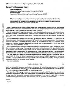
FIG. 1. Correlation functions of photon operators in compact U(1) lattice gauge theory at β ¼ 1.2 plotted versus Euclidean timestep t.
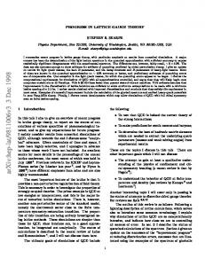
obtained, Fig. 1 shows the diagonal correlators at β ¼ 1.2 of the operators discussed in Sec. II projected with one unit of lattice momentum ( ⃗p ¼ π8 ð1; 0; 0Þ and permutations with momentum transverse to the vector operator). Energies were obtained using a constrained two-exponential fit [20] over the whole time range (excluding the source point). The results for β > βc are shown in Fig. 2 for operators projected with one and two lattice units of momentum. The dashed lines in the figure are the energies calculated using the lattice dispersion relation X 2 coshðEÞ ¼ m2 þ 8 − 2 cosðpi Þ ð9Þ i
with m2 ¼ 0. Below βc the photon operators propagate massive states. This can be inferred, e.g., from the momentum-projected correlation functions of O4 calculated at some values
of β just below the critical value and plotted in Fig. 3. The correlators survive only a few time steps before disappearing into noise so it is difficult to determine the asymptotic value of the ground state energy. However, the rate of falloff of the correlation functions where they are statistically significant would indicate a mass greater than one, i.e., larger than the cutoff scale. This is consistent with the results of Refs. [1,21]. To confirm that our set of four operators is providing evidence that the theory contains just one photon, we can study the full 4 × 4 correlation matrix of sources and sinks. First, the correlation function of O1 with any of the others is found to be statistically consistent with zero at every time step, as expected because O1 contains no T −− 1 component while the others are exclusively T −− . Next we consider all 1 elements of the 3 × 3 correlation matrix for O2, O3 and O4 . The normalization of each operator is chosen such that its diagonal correlator is unity at t ¼ 1 (which is right beside the source). This rescales all 9 elements of the correlation matrix as follows:
Energy [lattice units]
Cij ðtÞ Cij ðtÞ → pffiffiffiffiffiffiffiffiffiffiffiffiffiffiffiffiffiffiffiffiffiffiffiffiffi Cii ð1ÞCjj ð1Þ
O1 O2 O3 O4
0.5
0.45
0.35 2 β
2.5
ð10Þ
where i ∈ ð2; 3; 4Þ and j ∈ ð2; 3; 4Þ. The resulting correlation functions are shown in Fig. 4. Data sets in this plot have a small horizontal offset for clarity, but the main point is that all nine sets are essentially indistinguishable up to some overall minus signs. Mathematically, the plot says our correlation matrix is proportional to
0.4
1.5
16
FIG. 3. Momentum-projected correlation functions of O4 at β values just below βc ≈ 1.01 in compact U(1) lattice gauge theory.
0.55
1
12
t
0
3
FIG. 2. Energies extracted from correlators of photon operators in compact U(1) lattice gauge theory as a function of β. Lower points are for one unit of lattice momentum. Upper points are for two units. The dashed lines show energies calculated using the lattice dispersion relation for a massless particle.
1
B M¼@ 1
1 1
−1 −1
−1
1
C −1 A
ð11Þ
1
which has a pair of vanishing eigenvalues and a single eigenvalue equal to 3. The corresponding eigenvectors are
034502-3
PHYS. REV. D 98, 034502 (2018)
RANDY LEWIS and R. M. WOLOSHYN O2O2 O2O3 -O2O4 O3O2 O3O3 -O3O4 -O4O2 -O4O3 O4O4
Higgs κ
normalized correlator
1
confined
0
0.1
10
5
Coulomb
∞
0
β
15
t
FIG. 5.
FIG. 4. Entries in the 3 × 3 correlation matrix for O2, O3 and O4 in compact U(1) lattice gauge theory with one unit of momentum at β ¼ 2.
λ1 ¼ 0 ⇒ v1 ¼ O2 − O3 ;
ð12Þ
λ2 ¼ 0 ⇒ v2 ¼ O2 þ O3 þ 2O4 ;
ð13Þ
λ3 ¼ 3 ⇒ v3 ¼ O2 þ O3 − O4 :
ð14Þ
Calculations of the vi vj correlation functions confirm that all of them are statistically consistent with zero at every time step, except v3 v3 which alone retains the original photon signal from Fig. 4. Therefore the original operators Oi are all coupling to the same photon, and v3 is maximizing our overlap with that photon. IV. ABELIAN HIGGS MODEL As an application for the operators discussed in the previous section, we consider the Abelian Higgs model. The lattice action for this model is S ¼ SG þ Sφ where the gauge action was defined in Eq. (8) and
O5 ¼ Imφ� ðxÞUi ðxÞφðx þ ˆiÞ
ð16Þ
is considered here. Numerical simulations were carried out on 164 lattices for a range of κ values at fixed β ¼ 2, well above the critical β of the pure gauge theory. Although strictly speaking not an order parameter, the quantity X GðxÞ ¼ Re φ� ðxÞU μ ðxÞφðx þ μˆ Þ
ð17Þ
μ
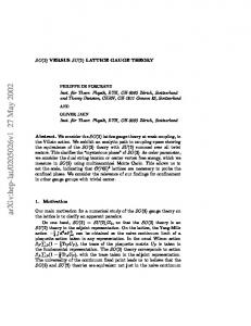
is used to locate the transition region from the Coulomb to the Higgs phase. The results are plotted in Fig. 6 where one can see that the critical κ is around 0.16. Diagonal correlators of the operators O1 to O4 projected with one unit of momentum were calculated for a range of κ values using a sample of 80 000 field configurations. Figure 7 showing the results at κ ¼ 0.145 illustrates the quality of the correlators. The energies extracted from diagonal photon correlators are plotted in Fig. 8. The dashed line in the figure shows the energy expected for a zero-mass particle. A massless photon exists in the Coulomb region
X ðφ� ðxÞU μ ðxÞφðx þ μˆ Þ þ H:c:Þ x;μ
X X þ φ� ðxÞφðxÞ þ λ ðφ� ðxÞφðxÞ − 1Þ2 : x
0.5
ð15Þ
0.4
x
The phase diagram at fixed λ is shown schematically in Fig. 5. Numerical calculations for this work were done assuming that the complex scalar field φ has a fixed unit norm, i.e., the value in the limit λ → ∞. In this limit only the hopping term of Sφ is needed and this saves some time in doing the simulation. The interest here is in showing the existence of a massless photon in the Coulomb phase and the fate of the photon in the Higgs region and we do not expect these qualitative aspects to depend on λ. In addition to the four operators discussed in previous sections, the composite vector boson operator
〈G(x)〉
Sφ ¼ −κ
Phase diagram of the Abelian Higgs model.
0.3 0.2 0.1 0
0.14
0.15
0.17
0.16
0.18
0.19
κ
FIG. 6. The expectation value of GðxÞ as a function of κ for the Abelian Higgs model at β ¼ 2 and λ ¼ ∞.
034502-4
PHYS. REV. D 98, 034502 (2018)
PHOTON OPERATORS FOR LATTICE GAUGE THEORY -3
-4
10
10
Correlation function
Correlation function
-4
O1 O2 O3 O4
10
-5
10
.160 .165 .170 .175 .180 .185 .190
-5
10
-6
10
-7
10 -6
10
0
4
8
12
0
16
4
8
FIG. 7. Correlation functions of photon operators in the Abelian Higgs model at κ ¼ 0.145, β ¼ 2 and λ ¼ ∞.
O1 O2 O3 O4
0.46 0.44
16
FIG. 9. Correlation functions of the composite vector operator O5 in the Abelian Higgs model at β ¼ 2 and λ ¼ ∞.
0.48
Energy [lattice units]
Energy [lattice units]
0.48
12
t
t
0.42 0.4 0.38
O5 O4
0.46 0.44 0.42 0.4
0.36 0.14
0.15
0.16
κ
0.17
0.18
0.38
0.19
0.17
FIG. 8. Energies extracted from correlators of photon operators projected with one unit of momentum in the Abelian Higgs model as a function of κ at β ¼ 2 and λ ¼ ∞. The dashed line shows energy calculated using the lattice dispersion relation for a massless particle.
but beyond κ ¼ 0.16 the increasing energies indicate an increasing nonzero mass. The correlation function of the composite boson operator O5 is plotted in Fig. 9 for κ values in the Higgs region. Near the transition the correlators are too noisy to obtain a reliable estimate of the ground state energy. At κ ¼ 0.175 and above, the ground state energy can be determined reasonably well and the values are shown in Fig. 10 for correlators projected with one unit of momentum. For comparison the energies extracted from the correlator of O4 are also shown. In the semiclassical treatment of the Abelian Higgs model, the massive vector boson appears as an elementary field [10] and it is natural to interpret it as a photon having acquired a mass. In contrast, nonperturbative lattice calculations typically use the gauge-invariant composite operator O5 to reveal the presence of a massive vector state [13]. As shown here there are photon interpolating
0.175
0.18
κ
0.185
0.19
0.195
FIG. 10. Energies extracted from the correlators of O5 and O4 in the Higgs region of the Abelian Higgs model.
operators which, when used in the Higgs region, exhibit a mass compatible with that of the composite vector boson. The question is whether the photon operators and the operator O5 are propagating the same state or not. To answer this question, cross correlations between different operators are needed. In previous studies [13] where only the simple plaquette operator O1 was considered, the mixing of the photon with the composite vector could not be addressed. Recall that operator O1 transforms as T þ− 1 and has no correlation with O5 which transforms as T −− 1 . What is different in this work is that operators with the appropriate photon transformation properties T −− have 1 been introduced so cross correlations can be studied. It was shown in Sec. III that the operators O2 , O3 and O4 all propagate the same photon state so, to study cross correlations with O5 , the operator O4 which has the smallest statistical fluctuations is chosen. Results will be shown here for κ ¼ 0.180. Other κ’s at 0.175 and above show similar behaviour. The four correlation functions
034502-5
PHYS. REV. D 98, 034502 (2018)
RANDY LEWIS and R. M. WOLOSHYN 44 55 45 54
-4
0.48
Energy [lattice units]
Correlation function
10
-5
10
-6
10
0.46
O5 O4 Eigenvalue 1
0.44 0.42 0.4
0
4
8
12
0.38
16
t
0.17
FIG. 11. The four correlation functions constructed from the operators O4 and O5 at κ ¼ 0.180.
(momentum projected) that can be constructed using operators O4 and O5 are shown in Fig. 11. It is apparent even without a quantitative fit that the diagonal correlator of O5 contains a substantial heavy non-ground state contribution which is not propagated by the photon operator O4. The cross correlators falling nicely in between the diagonal correlators is already an indication of the high degree of correlation between the operators. The eigenvalues of the 2 × 2 correlator matrix were calculated at every time step and are plotted in Fig. 12. The two eigenvalues are very different in magnitude and time dependence. The ground state energy extracted from the large eigenvalue is compatible with that extracted from the diagonal correlators alone. This is shown in Fig. 13 along with results for other κ values. The small eigenvalue is statistically significant only near the source and reflects the fact that O5 can excite some high lying states. This eigenvalue is too small to measure at larger time separations which is an indication that the operators O4 and O5 propagate the same ground state. This result reminds us -4
Correlator matrix eigenvalue
10
-5
10
-6
10
-7
10
-8
10
-9
10
0
4
8
12
16
t
FIG. 12. Eigenvalues of the 2 × 2 correlation matrix constructed from the operators O4 and O5 at κ ¼ 0.180. The triangles denote points where the eigenvalue is negative.
0.175
0.18
κ
0.185
0.19
0.195
FIG. 13. Energies extracted from the large eigenvalue of the 2 × 2 correlator matrix compared to values from the correlators of O5 and O4 in the Higgs region of the Abelian Higgs model.
that in the nonperturbative context the view that the massive vector boson present in the Higgs regime is a massive photon is too simplistic and does not account for the fact that in a field theory all allowable field configurations can contribute to physical states. V. SUMMARY Past studies of lattice theories containing U(1) gauge fields provided evidence of a massless photon in the theory’s unconfined phase without having a single-photon operator, relying instead on an operator for a pair of photons. Here we have constructed three different operators with single-photon transformation properties T −− 1 and used them to confirm the massless photon. The pattern of cross correlations among these operators shows that they are all propagating the same photon state. Our “solenoidal” operator (here called O4 ) was found to give a particularly robust signal for the photon. As a further application of the single photon operators we consider the fate of the photon in the Abelian Higgs model. Past lattice studies of this model have used a composite vector operator (here called O5 ) built from both the scalar and gauge fields to expose the presence of a massive vector particle in the Higgs regime. Now that we have T −− 1 operators built purely from gauge fields (O2 , O3 and O4 ), cross correlations can be studied and it was shown that the photon and composite vector operators couple to the same massive vector state. It was also observed that there is some excited state contribution present in the correlator of O5 which is absent from O2 , O3 and O4 . It may be interesting for future work to study these excited state effects in detail. The photon operators discussed in this work can be applied in other field theories. Of particular relevance may be SUð2Þ × Uð1Þ gauge theory with a complex Higgs doublet, where the photon, customarily understood to
034502-6
PHYS. REV. D 98, 034502 (2018)
PHOTON OPERATORS FOR LATTICE GAUGE THEORY emerge as a linear combination of the SU(2) and U(1) gauge fields, remains massless in the Higgs phase. The operators discussed here could be useful for investigating the lattice version of this scenario.
Canada. TRIUMF receives federal funding via a contribution agreement with the National Research Council of Canada. APPENDIX: EXPLICIT OPERATORS
ACKNOWLEDGMENTS The work of R. L. is supported in part by the Natural Sciences and Engineering Research Council of
The operators are constructed in a spatial lattice at a fixed Euclidean time. Using i, j, k to denote the 3 distinct spatial directions, the operators are
ˆ þ Pjk ðx − kÞÞ; ˆ ˆ þ Pjk ðx − jˆ − kÞ Oi1 ðxÞ ¼ ImðPjk ðxÞ þ Pjk ðx − jÞ
ðA1Þ
Oi2 ðxÞ ¼ ImðQij ðxÞ þ Qij ðx − ˆiÞ þ Qik ðxÞ þ Qik ðx − ˆiÞÞ;
ðA2Þ
Oi3 ðxÞ ¼ ImðRij ðxÞ þ Sij ðxÞ þ Rik ðxÞ þ Sik ðxÞÞ;
ðA3Þ
ˆ þ Pik ðx − ˆiÞ þ Pki ðx − ˆi − kÞÞ; ˆ ˆ þ Pij ðx − ˆiÞ þ Pji ðx − ˆi − jÞP ˆ ik ðxÞ þ Pki ðx − kÞ Oi4 ðxÞ ¼ ImðPij ðxÞ þ Pji ðx − jÞ
ðA4Þ
where ˆ †j ðxÞ; Pij ðxÞ ¼ Ui ðxÞUj ðx þ ˆiÞU †i ðx þ jÞU
ðA5Þ
ˆ †j ðx þ ˆiÞU †i ðxÞU†j ðx − jÞU ˆ i ðx − jÞU ˆ j ðx þ ˆi − jÞU ˆ †i ðxÞ; Qij ðxÞ ¼ U j ðxÞU i ðx þ jÞU
ðA6Þ
ˆ †j ðxÞU†j ðx − jÞU ˆ †i ðx − ˆi − jÞU ˆ j ðx − ˆi − jÞU ˆ i ðx − ˆiÞ; Rij ðxÞ ¼ Ui ðxÞUj ðx þ ˆiÞU †i ðx þ jÞU
ðA7Þ
ˆ †i ðx − jÞU ˆ j ðx − jÞU ˆ j ðxÞU†i ðx − ˆi þ jÞU ˆ †j ðx − ˆiÞUi ðx − ˆiÞ: Sij ðxÞ ¼ U i ðxÞU †j ðx þ ˆi − jÞU
ðA8Þ
Another option for operator O2 is given by ˆ þ Qij ðx − ˆi − jÞ ˆ þ Qij ðx þ jÞ ˆ þ Qij ðx − ˆi þ jÞ ˆ Oi2 ðxÞ ¼ ImðQij ðxÞ þ Qij ðx − ˆiÞ þ Qij ðx − jÞ ˆ þ Qik ðx − ˆi − kÞ ˆ þ Qik ðx þ kÞ ˆ þ Qik ðx − ˆi þ kÞÞ: ˆ þ Qik ðxÞ þ Qik ðx − ˆiÞ þ Qik ðx − kÞ
[1] B. Berg and C. Panagiotakopoulos, Phys. Rev. Lett. 52, 94 (1984). [2] I.-H. Lee and J. Shigemitsu, Phys. Lett. 169B, 392 (1986). [3] I.-H. Lee and J. Shigemitsu, Nucl. Phys. B276, 580 (1986). [4] H. G. Evertz, K. Jansen, J. Jersák, C. B. Lang, and T. Neuhaus, Nucl. Phys. B285, 590 (1987). [5] P. Majumdar, Y. Koma, and M. Koma, Nucl. Phys. 677, 273 (2004). [6] A. K. De and M. Sarkar, J. High Energy Phys. 10 (2017) 125. [7] R. M. Woloshyn, Phys. Rev. D 95, 054507 (2017). [8] B. Berg and A. Billoire, Nucl. Phys. B221, 109 (1983). [9] A. H. Guth, Phys. Rev. D 21, 2291 (1980). [10] P. W. Higgs, Phys. Rev. 145, 1156 (1966). [11] E. H. Fradkin and S. H. Shenker, Phys. Rev. D 19, 3682 (1979). [12] K. Jansen, J. Jersák, C. B. Lang, T. Neuhaus, and G. Vones, Phys. Lett. 155B, 268 (1985).
ðA9Þ
[13] K. Jansen, J. Jersák, C. B. Lang, T. Neuhaus, and G. Vones, Nucl. Phys. B265, 129 (1986). [14] V. Azcoiti, G. di Carlo, and A. F. Grillo, Phys. Lett. B 258, 207 (1991). [15] J. L. Alonso et al., Nucl. Phys. B405, 574 (1993). [16] M. Baig and J. Clua, Phys. Rev. D 57, 3902 (1998). [17] F. Romero-López, A. Rusetsky, and C. Urbach, Phys. Rev. D 98, 014503 (2018). [18] J. Jersák, T. Neuhaus, and P. M. Zerwas, Nucl. Phys. B251, 299 (1985). [19] G. Arnold, B. Bunk, T. Lippert, and K. Schilling, Nucl. Phys. B, Proc. Suppl. 119, 864 (2003). [20] G. P. Lepage, B. Clark, C. T. H. Davies, K. Hornbostel, P. B. Mackenzie, C. Morningstar, and H. Trottier, Nucl. Phys. B, Proc. Suppl. 106, 12 (2002). [21] A. Nakamura and M. Plewnia, Phys. Lett. B 255, 274 (1991).
034502-7