Physical Limits of Computing - CiteSeerX

To be published in the IEEE Computing in Science & Engineering magazine, May/June 2002. Draft of Feb. 14. References now in good shape. Still needs re-reviewed, and edited to length.

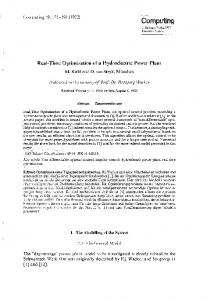
Physical Limits of Computing Michael P. Frank University of Florida, CISE Department February 14, 2002 Computational science & engineering and computer science & engineering have a natural and long-standing relation. Scientific and engineering problems tend to place some of the most demanding requirements on computational power, thereby driving the engineering of new bit-device technologies and circuit architectures, as well as the scientific & mathematical study of better algorithms and more sophisticated computing theory. The need for finitedifference artillery ballistics simulations during World War II motivated the ENIAC, and massive calculations in every area of science & engineering motivate the PetaFLOPSscale* supercomputers on today’s drawing boards (cf. IBM’s Blue Gene [1]). Meanwhile, computational methods themselves help us to build more efficient computing systems. Computational modeling and simulation of manufacturing processes, logic device physics, circuits, CPU architectures, communications networks, and distributed systems all further the advancement of computing technology, together achieving ever-higher densities of useful computational work that can be performed using a given quantity of time, material, space, energy, and cost. Furthermore, the long-term economic growth enabled by scientific & engineering advances across many fields helps make higher total levels of societal expenditures on computing more affordable. The availability of more affordable computing, in turn, enables whole new applications in science, engineering, and other fields, further driving up demand. Partly as a result of this positive feedback loop between increasing demand and improving technology for computing, computational efficiency has improved steadily and dramatically since computing’s inception. When looking back at the last forty years (and the coming ten or twenty), this empirical trend is most frequently characterized with reference to the famous "Moore’s Law" [2], which describes the increasing density of microlithographed transistors in integrated semiconductor circuits. (See figure 1.)34 Interestingly, although Moore’s Law was originally stated in terms that were specific to semiconductor technology, the trends of increasing computational density inherent in the law appear to hold true even across multiple technologies. One can trace the history of computing technology back through discrete transistors, vacuum tubes, electromechanical relays, and gears, and amazingly, we still see the same exponential curve extending across all these many drastic technological shifts. Furthermore, when looking back far enough, the curve even appears to be super-exponential; the frequency of doubling of computational efficiency appears to itself increase over the long term ([5], pp. 20-25). Naturally, we wonder just how far we can reasonably hope this fortunate trend to take us. Can we continue indefinitely to build ever more and faster computers using our available economic resources, and apply them to solve ever larger and more complex scientific and engineering problems? What are the limits? Are there limits? When *

Peta = 1015, FLOPS = FLoating-point Operations Per Second

semiconductor technology reaches its technology-specific limits, can we hope to maintain the curve by jumping to some alternative technology, and then to another one after that one runs out? ITRS Feature Size Projections 1000000 uP chan L DRAM 1/2 p

100000

min Tox

Human hair thickness

Feature Size (nanometers)

max Tox 10000

Eukaryotic cell

1000

Bacterium

Virus

100

Protein molecule

10

DNA molecule thickness

1

Atom 0.1 1955 1960 1965 1970 1975 1980 1985 1990 1995 2000 2005 2010 2015 2020 2025 2030 2035 2040 2045 2050 Year of First Product Shipment

We are here

Figure 1. Trends for minimum feature size in semiconductor technology. The data in the middle are taken from the 1999 edition of the International Technology Roadmap for Semiconductors [3]. The point at left represents the first planar transistor, fabricated in 1959 [4]. Presently, the industry is actually beating the roadmap targets that were set just a few years ago; ITRS targets have historically always turned out to be conservative, so far. From this data, wire widths, which correspond most directly to overall transistor size, would be expected to reach near-atomic size by about 2040-2050, unless the trend line levels off before then. It is interesting to note that in some experimental processes, some features such as gate oxide layers are already only a few atomic layers thick, and cannot shrink further.

Obviously, it is always a difficult and risky proposition to forecast future technological developments. However, 20th-century physics has given forecasters a remarkable gift, in the form of the very sophisticated modern understanding of physics, as embodied in the Standard Model of particle physics. Although of course many interesting unsolved problems remain in physics at higher levels, all available evidence tells us that the Standard Model, together with general relativity, explains the foundations of physics so successfully that apparently no experimentally accessible phenomenon fails to be encompassed within it at present. That is to say, no definite and persistent inconsistencies between these fundamental theories and empirical observations have been uncovered in physics within the last couple of decades. And furthermore, in order to probe beyond the range where the theory has already been thoroughly verified, physicists find that they must explore subatomic-particle energies above a trillion electron volts, and length scales far tinier than a proton’s radius. The few remaining serious puzzles in particle physics, such as the masses of particles, the disparity between the strengths of the fundamental forces, and the unification of general relativity and quantum mechanics are of a rather abstract and aesthetic flavor. Their eventual resolution (whatever form it takes) is not currently expected to have any

significant applications until one reaches the highly extreme regimes that lie beyond the scope of present physics (although, of course, we cannot assess the applications with certainty until we have a final theory). In other words, we expect that the fundamental principles of modern physics have "legs," that they will last us a while (many decades, at least) as we try to project what will and will not be possible in the coming evolution of computing. By taking our best theories seriously, and exploring the limits of what we can engineer with them, we push against the bounds of what we think we can do. If our present understanding of these limits eventually turns out to be seriously wrong, well, then the act of pushing against the limits is probably the activity that is most likely to lead us to that very discovery. (This methodological philosophy is nicely championed by Deutsch [6].) So, I personally feel that forecasting future limits, even far in advance, is a useful research activity. It gives us a roadmap showing where we may expect to go with future technologies, and helps us know where to look for advances to occur, if we hope to ever circumvent the limits imposed by physics, as it is currently understood. Interestingly, just by considering fundamental physical principles, and by reasoning in a very abstract and technology-independent way, one can arrive at a number of firm conclusions about upper bounds, at least, on the limits of computing. I have furthermore found that often, an understanding of the general limits can be applied to improve one’s understanding of the limits of specific technologies. Let us now review what is currently known about the limits of computing in various areas. Throughout this article, I will focus primarily on fundamental, technologyindependent limits, since it would take too much space to survey the technology-specific limits of the many present and proposed future computing technologies. But first, before we can talk sensibly about information technology in physical terms, we have to define information itself, in physical terms. Physical Information and Entropy From a physical perspective, what is information? For purposes of discussing the limits of information technology, the relevant definition relates closely to the physical quantity known as entropy. As we will see, entropy is really just one variety of a more general sort of entity which we will call physical information, or just information for short. (This abbreviation is justified because all information that we can manipulate is ultimately physical in nature [7].) The concept of entropy was introduced in thermodynamics before it was understood to be an informational quantity. Historically, it was Boltzmann who first identified the maximum entropy S of any physical system with the logarithm of its total number of possible, mutually distinguishable states. (This discovery is carved on his tombstone.) I will also call this same quantity the total physical information in the system, for reasons to soon become clear. In Boltzmann’s day, it was a bold conjecture to presume that the number of states for typical systems was a finite one that admitted a logarithm. But today, we know that operationally distinguishable states correspond to orthogonal quantum state-vectors, and the number of these for a given system is well-defined in quantum mechanics, and furthermore is finite for finite systems (more on this later).

Now, any logarithm, by itself, is a pure number, but the logarithm base that one chooses in Boltzmann’s relation determines the appropriate unit of information. Using base 2 gives us the information unit of 1 bit, while the natural logarithm (base e) gives us a unit I like to call the nat, which is simply (log2 e) bits. In situations where the information in question happens to be entropy, the nat is more widely known as Boltzmann’s constant kB. Any of these units of information can also be associated with physical units of energy divided by temperature, because temperature itself can be defined as just a measure of energy required per increment in the log state count, T = ∂E/∂S (holding volume constant). For example, the temperature unit 1 Kelvin can be defined as a requirement of 1.38 × 10-23 Joules (or 86.2 µeV) of energy input per increase of the log state count by 1 nat (that is, to multiply the number of states by e). A bit, meanwhile, is associated with the requirement of 9.57 × 10-24 Joules (59.7 µeV) energy per Kelvin that is needed to double the system’s total state count. Now, that’s information, but what distinguishes entropy from other kinds of information? The distinction is fundamentally observer-dependent, but in a way that is well-defined, and that coincides for most observers in simple cases. Let known information be the physical information in that part of the system

Physical Information Known information plus entropy = maximum entropy = maximum known information

Example:

1 2 3

System with 3 twostate subsystems, such as quantum spins.

23=8 states Known Information

Entropy

Spin label 1 2 3

Informational Status Entropy Known information Entropy

Figure 2. Physical Information, Entropy, and Known Information. Any physical system, when described only by constraints that upper-bound its spatial size and its total energy, still has only a finite number of mutually distinguishable states consistent with those constraints. The exact number N of states can be determined using quantum mechanics (with help from general relativity in extreme-gravity cases). We define the total physical information in a system as the logarithm of this number of states; it can be expressed equally well in units of bits or nats (a nat is just Boltzmann’s constant kB). In the example at right, we have a system of 3 two-state quantum spins, which has the 23=8 distinguishable states shown. It therefore contains a total of 3 bits = 2.08 kB of physical information. Relative to some knowledge about the system’s actual state, the physical information can be divided into a part that is determined by that additional knowledge (known information), and a part that is not (entropy). In the example, suppose we happen to know (through preparation or measurement) that the system is not in any of the 4 states that are crossed out (i.e., has 0 amplitude in those states). In this case, the 1 bit (0.69 kB) of physical information that is associated with spin number 2 is then known information, whereas the other 2 bits (1.39 kB) of physical information in the system are entropy. The available knowledge about the system can change over time. Known information becomes entropy when we forget or lose track of it, and bits of entropy can become known information if we measure them. However, the total physical information in a system is exactly conserved, unless the system’s size and/or energy changes over time (as in an expanding universe, or an open system).

NonUniform vs. Uniform Probability Distributions

Probability

Odds (Inverse Probability)

1

80

0.8

Odds 60 Against (1 out of N)

0.6

40

0.4

20

0.2

0

0 1

2

3

4 State

5

6

7

8

9

1 2 3 4 5 6 7 8 9 10 State

10

Log Odds (Information of Discovery)

7 6 5 Log Base 2 4 3 of Odds 2 1 0

Shannon Entropy (Expected Log Odds) 0.5 0.4 Bits

0.3 0.2 0.1 0

1 2 3 4 5 6 7 8 9 10 State

1 2 3 4 5 State Index

6

7

8

9 10

Figure 3. Shannon Entropy. The figure shows an example of Shannon’s generalization of Boltzmann entropy for a system having ten distinguishable states. The blue bars correspond to a specific nonuniform probability distribution over states, while the purple bars show the case with a uniform (Boltzmann) distribution. The upper-left chart shows the two probability distributions. Note that in the nonuniform distribution, we have a 50% probability for the state with index 4. The upper-right chart inverts the probability to get the odds against the state; state 4 is found in 1 case out of 2, whereas state 10 (for example) appears in 1 case out of 70. The logarithm of this "number of cases" (lower left) is the information gain if this state were actually encountered; in state 4 we gain 1 bit; in case 10, more than 6 bits (26=64). Weighting the information gain by the state probability gives the expected information gain. Because the logarithm function is concave-down, a uniform distribution minimizes the expected log-probability, maximizes its negative (the expected log-odds, or entropy), and minimizes the information (the expected log-probability, minus that of the uniform distribution).

whose state is known (by a particular observer), and entropy be the information in the part that is unknown. The meaning of "known" can be clarified, by saying that a system A (the observer) knows the state of system B (the observed system) to the extent that some part of the state of A (e.g. some record or memory) is correlated with the state of B, and furthermore that the observer is able to access and interpret the implications of that record regarding the state of B. To quantify things, the maximum known information or maximum entropy of any system is, as already stated, just the log of its possible number of distinguishable states. If we know nothing about the state, all the system’s physical information is entropy, from our point of view. But, as a result of preparing or interacting with a system, we may come to know (or learn) something more about its actual state, besides just that it is one of the N states that were originally considered "possible." Suppose we learn that the system is in a particular subset of M