Plankton Classification Using Hybrid Convolutional Network-Random Forests Architectures Pranav Jindal Department of Computer Science, Stanford University
[email protected]
Rohit Mundra Department of Electrical Engineering, Stanford University
[email protected]
Abstract
1.2. Dataset The data provided by Kaggle for the competition consisted of labeled training images and unlabeled test images which were in grayscale although they were stored in 3channel JPEG images. Since the images were acquired from an underwater towed imaging system, they were segmented by the competition hosts such that each image contained just one species of plankton. As a result, the images were distributed unevenly among 121 classes and were of different dimensions ranging from as little as 40 pixels to as much as 400 pixels in one dimension. The exact number of images for training and test are listed here.
Convolutional Neural Networks have been established as the dominant choice for recent state-of-art image classification systems. Encouraged by their success at both image classification and feature extraction, we attempt to use CNNs to work on the image classification task of automatically identifying different species of plankton. We approach the problem by first directly applying CNNs to classify the plankton and move progressively towards using CNNs as a generic feature extractor with a random-forest classifier on top of the hierarchy. We examine the performance of both the above approaches and discuss the results obtained in the Kaggle National Data Science Bowl 2015.
Training/Labeled Test/Unlabeled
30,336 images 130,400 images
It is visible that the training set is substantially smaller than the test set and thus, in the next section we describe data augmentation to inflate the training set size.
1. Introduction In this section we describe the problem trying to be addressed by the National Data Science Bowl 2015 along with the dataset.
1.1. Problem This paper focuses on the automated classification of 121 types of plankton for the National Data Science Bowl presented by Kaggle and Booz Allen Hamilton. Planktons are vital for our ecosystem as they account for more than half the primary productivity on earth and nearly half the total carbon fixed in the global carbon cycle. Loss of plankton populations can have devastating impacts in our ecosystem and thus, measuring and monitoring them is fundamental to the wellbeing of our society. Conventional methods for measuring and monitoring plankton populations are infeasible and do not scale well - they involve analysis of underwater imagery by an expert at plankton recognition. The automation of this task will have broad applications for assessment of ocean and ecosystem health.
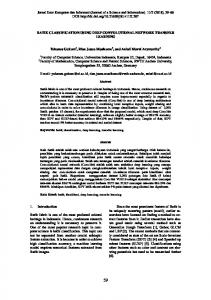
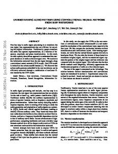
Figure 1. Plankton varieties
Some examples of labeled plankton images are shows in Figure 1. 1
2. Preprocessing and Data Augmentation In this section, we describe the preprocessing steps and data augmentations training and test images underwent before being used for training.
2.1. Dimensional Uniformity The dataset provided by Kaggle consists of images of varying sizes, however conventional CNNs require that all the input images have the same dimensions. Since the image sizes ranged from 40 pixels to 400 pixels wide, we decided to work with 128 × 128 pixel images. Even so, most images did not have a 1 : 1 aspect ratio and we decided to experiment with two approaches: 1. Maintaining aspect ratio: This involves making sure the larger of the two dimensions of a given image is scaled such that it is 128 pixels shaped in that dimension. The smaller of the two dimensions would obviously scale down by maintaining aspect ratio to less than 128 pixels. The resulting space which does not represent the image (due to the smaller dimension being less than 128 pixels) is left to have a white background since it blends well with backgrounds of images. 2. Forgoing aspect ratio: This involves forcing every image (regardless of original dimensions) to be scaled to fit 128×128 in each dimension. As a result, this causes many images (particularly rectangular ones) to appear distorted.
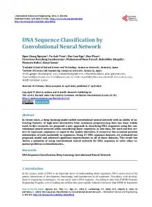
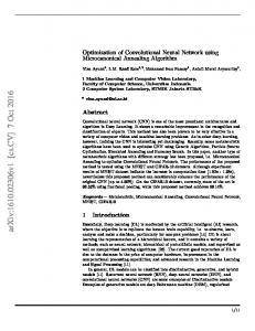
Figure 2. Canny-edge detection on original images
2.3. Data Augmentations Since the test data was substantially larger than the training data, it was difficult to generalize well without artificially inflating the dataset by using augmentations. As a result, we tried many data augmentations: 1. 2. 3. 4. 5.
On training convolutional networks (described in later sections) with both types of transformations described above, we found little to no difference in training and validation loss and decided to preserve the aspect ratio for one of our convolutional networks (ClassyFireNet) and forgo the aspect-ratio for the other net (GoogLeNet).
Rotation (0◦ to 360◦ with 20◦ increments) Zooming (factors of 1/1.3, 1/1.2, 1/1.1, 1.1, 1.2, 1.3) Shearing (−20◦ and 20◦ ) Flipping (Bernoulli, p = 0.5) Translation (+/ − 4 pixels randomly offset in x and y directions, each with uniform probability)
Even though real-time data augmentation almost always outperforms offline/batch-processing data augmentation, we were constrained to use offline data augmentation for rotation, zooming and shearing since Caffe, our deep-learning framework, does not facilitate real-time data augmentation of these types. It does however provide real-time data augmentation for flipping and translation so these were done in real-time.
2.2. Filtering Images As part of the experimentation, we also tried applying the canny-edge detector on the original images and fed the resultant edge-images for training. Our motivation was that a much of the noise present in the images would be removed as a result of this transformation. However, we found that this filter on this dataset did not perform better than the raw images. We hypothesize that this is a result of the loss of texture from plankton images causing convolutions to be less effective. Figure 2 shows examples of the original images as well as the transformation after applying the canny-edge detector on the image.
2.4. Training/Validation Split We decided to use 85% of the original dataset for training purposes and the remaining 15% for validation. The datapoints were chosen randomly and even though stratification was not enforced, both sets were verified to be representative of the original class distribution. It is important to note that if a given image was used for training, so were all its augmentations. This prevented the use of an image for training and its transformation for validation – a situation likely to lead to over-optimistic validation loss. 2
3. Loss Function
troducing a network with relatively few convolutional layers and describe how we progressed to deeper networks.
This section describes the loss functions being minimized by the convolutional networks as well as random forests. This is vital to understand since changes in loss functions change the fundamental optimization objective for a classifier.
4.1. Phase 1: 4 convolution, 1 fully-connected layers As our first attempt to training CNNs for the competition, we started with a very simple network with just 4 convolutional layers (conv3-64 each) and 1 fully connected layer (FC-256) leading to a 121 class Softmax prediction. This network was not trained over GPUs but instead over an Intel Architecture 64-bit CPU. The network training lasted over 24 hours resulting in the training and validation losses to saturate around 1.58. Since the training loss and validation losses were not disparate, we realized that our model had very low capacity and overfitting was not possible even without data augmentations. Thus, we realized our next step was to use a deeper model with more capacity.
3.1. Logarithmic Loss The primary metric for evaluation for this competition was log-loss calculated over all test examples in the following manner: logloss = −
N M 1 XX yij loge (pij ) N i=1 j=1
4.2. Phase 2: 5 convolution, 2 fully-connected layers
N = Number of test examples (130,400) M = Number of classes (121) pij = Predicted probability of test example i belonging to class j yij = 1 if test example i does indeed belong to class j, else 0. Intuitively, a small loss indicates that the classifier (on average) predicts a high probability of the correct class. For instance, if the classifier predicted an image to belong to the correct class with probability of 0.25, the logloss would then be − loge (0.25) = 1.386. Conversely, if a logloss of 1.386 is experienced over a dataset, one can infer that the classifier predicted the correct class to have probability of e−1.386 = 0.25 on average. A consequence of using this loss metric is that assigning very low probabilities for the correct class even a few times over the entire dataset can be very expensive. Since this was the metric the competition assessments were made on, our convolutional networks minimized this loss function.
In our second design phase, we decided to use a deeper network than that used in Phase 1. To get started, we used the default CaffeNet architecture provided by the Caffe framework. The only modifications were only those in the input and output layers (data size and number of classes). Data (128 × 128) Conv11-96 (Stride 4) Maxpool3 (Stride 2) LRN-5 Conv5-256 Maxpool3 (Stride 2) LRN-5 Conv3-384 Conv3-384 Conv3-256 Maxpool3 (Stride 2) FC-512 Dropout (0.5) FC-512 Dropout (0.5) Softmax-121
3.2. Classification Rate Another useful and popular metric for classification problems is the classification rate – the fraction of data points for which the maximum probability (over all classes) is assigned to the correct class. This loss metric is invariant to the actual value of the probability assigned to the correct class and only checks whether the correct class is assigned a higher probability than all others. While this metric is not used for optimization purposes in the convolutional network training, it is the default metric used for Random Forests training.
The above network was first trained on just the training data and was found to overfit after 13-14 epochs of training. This training lasted 6-8 hours on an NVIDIA Grid K520 GPU and resulted in a training loss of 0.81 with a validation loss of 1.18. We also tried removing the local response normalization layers and found no difference in performance. Since we had managed to overfit even in presence of dropout layers, we tried reducing the gap between training and testing losses by adding rotated images as data augmentation. We added 45◦ increment rotations of each image thereby increasing the total dataset by a factor of 7. We transferred our previously overfit model and retrained on
4. Network Architecture This section describes the evolution the convolutional networks we used in a step-wise manner. We start with in3
4.4. Phase 3b: GoogLeNet[5]
the new dataset for nearly 10 epochs of the new augmented dataset. This resulted in both, the training and validation losses, to saturate at 0.94. Since we had again arrived at a situation where our training and validation loss were similar, we decided to move to even deeper networks to increase our model capacity further.
Motivated by the recent introduction of multi-scale convolutional networks, we trained a naive and modified implementation of the GoogLeNet as described in [5]. By naive, we imply that certain optimizations such as batch normalization were not used. Furthermore the weights were also initialized using the Xavier algorithm [1] as opposed to using gaussian. The modifications made were to use an 8 × 8 kernel for the first convolution layer and the last average pooling layer and the removal of the first max-pool layer. Of course, we also changed the Softmax layer to output 121 classes instead of 1000 classes (ImageNet). These changes allowed us to work with 128 × 128 pixel images and predict over the 121 different plankton classes. Using augmentations similar to those in Phase 3a, we were able to achieve a validation performance of 0.817 using this model on our dataset. Submitting the predictions of this model to Kaggle, we realized a test loss of 0.798.
4.3. Phase 3a: ClassyFireNet – 8 conv, 2 FC This was the first part of our final convolutional network design phase. Here we designed a network influenced some of the models proposed in [2]. The key idea behind the design of this model was to start with identifying low level features in the earlier levels with 3 × 3 convolutions build higher level features with greater depth later. The architecture we used is tabulated below and is called the ClassyFireNet. Data (128 × 128) Conv3-64 Maxpool Conv3-128 Conv3-128 Maxpool Conv3-256 Conv3-256 Maxpool Conv3-512 Conv3-512 Maxpool FC-512 Dropout (0.5) FC-512 Dropout (0.5) Softmax-121
5. Training This section describes the general strategy for training and avoiding overfitting (a recurring issue in convolutional networks in presence of limited data) along with some details of training algorithm used.
5.1. Training Algorithm We trained all our models using mini-batch stochastic gradient descent with Nesterov momentum as described in [4]. The batch size varied for different models depending on GPU memory constraints but typically varied between 32 to 64 training examples. Since the batch sizes were relatively small compared to the size of the dataset, a momentum of 0.9 was found to help reduce fluctuations in training. All our model parameters were initialized using the Xavier algorithm for initialization as discussed in [1]. We used a learning rate of 0.01 at the start of each model and stepped down to a factor of 0.9 after 10 epochs of the original dataset ( 303,360 images). At many instances, the learning rate was decreased to smaller values by intervening between training when we noticed that the validation loss stopped changing. The learning rate mentioned above was that for the non-bias weights. Bias weights learned at 2× rate.
Training the architecture above without any data augmentations, we were able to overfit very quickly. This was expected considering the architecture in Phase 2 overfit rather easily as well in the absence of augmentations. To recover from overfitting, we added rotations (20◦ increments) as a data augmentation along with translation (+/ − 4 pixels randomly offset in x and y directions, each with uniform probability) and flipping (Bernoulli, p = 0.5). We resumed training on the previously learned weights for the network for 5-10 more epochs (epochs of augmented dataset). As such, we managed a validation loss of 0.83 with a training loss of 0.62. To further reduce overfitting, we introduced more augmentations such as zooming (factors of 1/1.3, 1/1.2, 1/1.1, 1.1, 1.2, 1.3) and shearing. Again, we resumed training from the previous best model and found the validation loss to be 0.794. We proceeded with a submission to Kaggle using this model and found a test loss of 0.785.
5.2. Regularization Since a large part of performance was to introduce ways of reducing overfitting, we considered many approaches. Firstly, adding data augmentations was found to reduce the gap between training and validation loss by improving validation performance. However, many times this was insufficient was generalization. Thus, we had drop-out layers in place after the fully connected layers to regularize the model further. A drop out value of 0.5 was found to perform best 4
in ClassyFireNet while dropout values of 0.4 and 0.6 were found to be better in the GoogLeNet model. We also experimented with the weight decay values ranging from 0.01 to 0.00001 to regularize further and found a weight decay value of 0.0001 to perform best.
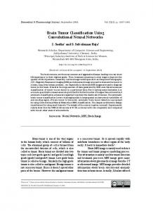
5.3. Strategy The strategy we used for training regardless of model can be succinctly put in the following way: 1. Design a convolutional network 2. Train without any data augmentations 3. If no overfitting occurs, end training and design a deeper convolutional network 4. If overfitting does occur, sequentially introduce data augmentations and resume training (See Figure 4). 5. After best augmentations have been identified, tune hyper-parameters (such as learning rate and weight decay) and resume training
Figure 4. CNNs as feature extractors
The features generated above were then used as training data along with the true labels for a random forests classifier. This idea can be seen in Figure 4 and has also been explored in recent works – for instance, for plant classification [3]. We found that with tree depths of 20-25 and with 10-100 trees, we were able to achieve very high validation classification rates using the random forests classifier (7677%). In comparison, our top two convolutional networks had classification rates of 71-74%. However, we found that the logloss of predictions from the random forests was substantially worse (around 0.92). This was understandable since the optimization problem solved by random forests is one that minimizes misclassification rate and not logloss. We found that the cause of high logloss was the extremely low probabilities being assigned to the correct class in instances where the classification was wrong. To abate this, we increased number of trees in the random forest to 500. While this did not change the classification rate much, it did improve the performance substantially resulting in a logloss of 0.81. The improvement was intuitive since 500 trees were more likely to assign non-zero probabilities to all 121 classes than were 100 trees.
Figure 3. Reducing overfitting using data augmentations
6. Feature Generation for Random Forests
7. Model Averaging
After we created the two convolutional networks described above, each with logloss near 0.80, we decided to try using our convolutional networks just for feature generation. We extracted the 512 features from the first fully connected layer (post-ReLU) from the ClassyFireNet for our entire training dataset. Similarly, we also extracted features from the GoogLeNet’s fully connected layer.
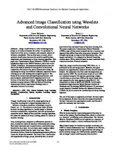
At this point, we had three sets of predictions, each with similar performance. However, our motivation behind using random forests was that an if − else type of classifier will make predictions quite different from those coming from a fully connected neural network. The diversity of predictions is crucial for ensembles to be successful. 5
On analysis of our predictions, we found this hypothesis to true. For instance Figure 5 shows the number of test examples that had their maximum probability (over all 121 classes) assigned to a given value between 0 and 1. We see that the random forests has far more examples where the maximum probability is less than 0.5 while the ClassyFireNet CNN has far more examples where the maximum probability is higher than 0.5. Given that both predictions have nearly the same logloss, this plot indicates presence of diversity between the two models’ predictions. We also measured the number of examples in which both methods predicted the same class to be more likely than any others and found that in 86% of the examples, the methods agreed on the classification. This again indicates the presence of diversity in the two models and thus motivates averaging between the two methods. We tried multiple types of ensembles. By ”Mean”, we imply that the probabilities were averaged for each class for each data point. By ”Max”, we imply that whichever model had a higher maximum probability (over all classes) was used for each data point. The different ensembles tried were: 1. ClassyFireNet + GoogLeNet (Mean) 2. ClassyFireNet + GoogLeNet (Max) 3. Random Forests + ClassyFireNet (Mean) 4. Random Forests + GoogLeNet (Mean) 5. Random Forests + ClassyFireNet (Max) 6. Random Forests + GoogLeNet (Max) 7. Random Forests + ClassyFireNet + GoogLeNet (Mean) 8. Random Forests + ClassyFireNet + GoogLeNet (Max) We found that our best test performance was when we used the mean of the random forests’ and ClassyFireNet’s predictions.
work, we achieved a logloss of 0.75. However, this result was achieved after the deadline of the competition and thus our best rank (out of 1049 contestants) at the end of the competition was 125 (logloss 0.77, top 12%) and after it ended was 103 (logloss 0.75, top 10%).
Figure 6. Team Classy Fire’s best entry on Kaggle
We learned from winners of the competition (logloss 0.56) that in presence of real-time data augmentation, our performance could have been even better. There is even room for more experimentation with the use of leaky ReLU units instead of ReLU units along with additional pooling techniques. Another area of exploration could be the use of other classifiers on the features extracted from the CNNs, such as Support Vector Machines (SVMs) and Gradient Boosting Machines (GBMs). For instance, GBMs have the advantage of variable optimization objectives (e.g. we can minimize logloss directly), however the trees require to be sequentially generated and are thus, slow to train.
References [1] X. Glorot and Y. Bengio. Understanding the difficulty of training deep feedforward neural networks. In International conference on artificial intelligence and statistics, pages 249–256, 2010. [2] K. Simonyan and A. Zisserman. Very deep convolutional networks for large-scale image recognition, 2014. [3] N. Sunderhauf, C. McCool, B. Upcroft, and P. Tristan. Finegrained plant classification using convolutional neural networks for feature extraction. In Working notes of CLEF 2014 conference, 2014. [4] I. Sutskever, J. Martens, G. Dahl, and G. Hinton. On the importance of initialization and momentum in deep learning. In Proceedings of the 30th International Conference on Machine Learning (ICML-13), pages 1139–1147, 2013. [5] C. Szegedy, W. Liu, Y. Jia, P. Sermanet, S. Reed, D. Anguelov, D. Erhan, V. Vanhoucke, and A. Rabinovich. Going deeper with convolutions, 2014.
Figure 5. CNNs as feature extractors
8. Results and Conclusions As a result of model averaging between predictions of random forests and the ClassyFireNet convolutional net6