Author's personal copy
Computer-Aided Design 43 (2011) 1099–1109
Contents lists available at ScienceDirect
Computer-Aided Design journal homepage: www.elsevier.com/locate/cad
Pocketing toolpath computation using an optimization method✩ Michel Bouard, Vincent Pateloup ∗ , Paul Armand Research institut XLIM - UMR CNRS 6172, Limoges, France
article
info
Article history: Received 8 September 2010 Accepted 28 May 2011 Keywords: Toolpath computation Optimization Pocket machining High-speed machining
abstract This paper proposes a new method of pocketing toolpath computation based on an optimization problem with constraints. Generally, the calculated toolpath has to minimize the machining time and respect a maximal effort on the tool during machining. Using this point of view, the toolpath can be considered as the result of an optimization in which the objective is to minimize the travel time and the constraints are to check the forces applied to the tool. Thus a method based on this account and using an optimization algorithm is proposed to compute toolpaths for pocket milling. After a review of pocketing toolpath computation methods, the framework of the optimization problem is defined. A modeling of the problem is then proposed and a solving method is presented. Finally, applications and experiments on machine tools are studied to illustrate the advantages of this method. © 2011 Elsevier Ltd. All rights reserved.
1. Introduction This article proposes a new method of toolpath computation using uniform cubic B-spline curves calculated with an optimization algorithm to describe the geometry of the path. The purpose of this methodology is to calculate C 2 -continuous cutting passes adapted to high-speed milling. This method is particularly dedicated to the calculation of pocketing toolpaths for aeronautical parts in aluminum, where the objective is to machine all the material within boundaries in a minimum time. Whereas all current methods of computation do not use optimization to generate the toolpath, our method proposes considering the calculation of each cutting pass as an optimization problem in which the objective is to minimize the machining time and the constraints consist of checking the cutting forces. The aim of pocket machining operations is to remove all the material inside a pre-defined contour between two horizontal planes in a minimal machining time. The only constraint specified by the part geometry is the boundary of the pocket [1]. Using this observation, any computed toolpath can take any shape if the pocket boundary is respected, the cutting conditions related to the tool/material are verified, and the removal of all the material inside the boundary is checked. Therefore, it can be interesting to compute a toolpath that fulfills the specifications quoted before and produces a minimal machining time by using the free form of the shape generated by the pocketing goal.
✩ This work is supported by the ‘‘Agence Nationale de la Recherche’’ under the reference ANR-08-JCJC-0038-01. ∗ Corresponding author. Tel.: +33 5 55 43 44 17. E-mail addresses:
[email protected] (M. Bouard),
[email protected] (V. Pateloup),
[email protected] (P. Armand).
0010-4485/$ – see front matter © 2011 Elsevier Ltd. All rights reserved. doi:10.1016/j.cad.2011.05.008
A review of pocket toolpath computation methods is presented by Hatna [1]. Generally, the machining strategy is based on the construction of parallel passes or offset curves at the boundary of the pocket (Fig. 1). If exclusively down-cut or up-cut milling is expected, contour-parallel toolpaths are preferred to directionparallel toolpaths in order to minimize the machining time [2]. The offset curves are calculated using a Voronoï diagram [3,4], a pair-wise offset algorithm [5], or a pixel-based approach [6]. A recent approach to compute offset curves not depending on the tool geometry has been developed by Molina [7]. It is based on the morphology of the external profile and avoids the main problems of traditional methods such as intersections, discontinuity, and lack of generality. All these methods compute pocket toolpaths using geometrical rules without optimization. Our previous studies [8,9] have improved these methods by using some possibilities offered by the free form of the toolpath inside the boundary. First, a method that increases the curvature radii at each corner of the toolpath was presented [8]. Then, a cubic Bspline interpolation of the cutting passes, based on the interpolation of circle arcs and straight lines, was developed to compute C 2 -continuous toolpaths [9]. With these two ‘‘add-ons’’, a classical toolpath can be improved by adding circle arcs at each corner and making it C 2 -continuous. Radii are calculated to check the maximum distance between cutting passes (dpmax ), which controls the radial depth of cut of the tool [8]. The B-spline interpolation is done to satisfy a maximum error chosen by the operator. Our approach is built on the fact that a pocket milling is considered as an optimization process of material removal under constraints. In this case, toolpath computation is not the result of a sequence of geometrical operations but the result of an optimization problem. This article is structured as follows. Initially, typical toolpath computation methods are analyzed. Our optimization method
Author's personal copy
1100
M. Bouard et al. / Computer-Aided Design 43 (2011) 1099–1109
Fig. 1. Usual pocket toolpaths.
Fig. 2. Usual pocket toolpaths for high-speed machining.
is then presented and compared to existing works. Experimental machine applications are presented to evaluate the benefits.
• Computation of the offset curves of the boundary curve using a
2. Definition of the optimization problem for pocketing toolpath computation
eliminate the non-machined areas and removal of the loops to decrease the toolpath length. • Creation of the toolpath linking using segments in order to minimize the toolpath length [10]. A toolpath linking is added between two successive offset curves. • Corner adaptation using circle arcs to replace right-angle corners in order to generate a G1 -toolpath.
To define the framework of the optimization problem, a study of classical pocketing toolpath computation methods is presented and analyzed. Then, the optimization problem is presented and compared to existing works. 2.1. Usual methods for pocketing toolpath computation A pocket machining can be defined as any machining which removes all the material located inside a preset boundary between two horizontal planes. The final part is obtained by the movement of the tool, according to the following constraints.
• Cutting constraint: efficient machining conditions have to be
used. Down-cut machining is especially expected for machining aeronautical parts in aluminum. • Mechanical constraint: the cutting efforts and cutting power consumed must be lower than the possible maximum limits of the machine and the tool. • Geometrical constraint: the machined boundary and the machined plane must respect the required dimensional specifications, shape deviation, and surface roughness. • Geometrical constraint: the internal area of the pocket must be completely machined. To satisfy these constraints, the toolpath is usually calculated using an algorithm for offset curve computation, which makes it possible to calculate a helical toolpath from the interior to the pocket outside or vice versa (Fig. 1). In the case of high-speed machining (HSM), Choi defines six stages in order to describe the computation of a pocketing toolpath using parallel contours [6].
• Determination of the boundary curve using the intersection of a plane perpendicular to the tool axis with the profile of the pocket.
pixel-based approach.
• Detection of the non-machined areas. • Fitting of the various elementary paths: addition of segments to
As a result, the calculated toolpath is illustrated in Fig. 2. The toolpath presents a set of discontinuities in curvature at each corner and at each toolpath linking. Indeed, a corner adaptation replaces one discontinuity in tangency by two discontinuities in curvature at the connects between circle arcs and straight lines. To fulfill the objective of minimizing the machining time, two ways of improvement can be explored. The first is based on the decrease of the length of the toolpath considering that the machining is realized at constant feedrate if the programmed one is low (Vf < 1 m/min). It is based on the following:
• the choice of the machining direction in ‘‘zigzag’’ mode [11,12], • the detection of the non-machined areas and their reduction in the case of a machining by contour-parallel offsets [13,14], and
• the optimization of the number and position of the connections between cutting passes [10].
The second considers that the real feedrate is never constant when the programmed one is high (Vf > 1 m/min). In this case, the real feedrate can be improved while respecting the constraints expressed above, by changing the geometry of the toolpath [8,15]. The main problem comes from each geometrical discontinuity of a toolpath that generates the following:
• a crossing with a high decrease of the feedrate if the toolpath is discontinuous in tangency [16],
• a reduction of the real feedrate of the tool in order to respect the contour error,
• dynamic loads on the machine tool structure during accelerations and decelerations,
Author's personal copy
M. Bouard et al. / Computer-Aided Design 43 (2011) 1099–1109
• a variation of the cutting conditions because of the variations of the feedrate, and • an increase in machining time due to the feedrate reduction.
Some methods that remove these discontinuities are proposed by computer-aided manufacturing (CAM) software. They are based on the use of circle arcs to remove tangency discontinuities and polynomial interpolation of the toolpath to remove curvature discontinuities. Hence, we can say that the shape of the computed toolpath directly influences the machining time. Thus the pocketing improvement needs to use new toolpath geometries. Some other authors use this approach [17,18]. Held proposes a method that generates a smooth G1 -toolpath. It is based on the placement of growing M-disks on the medial axis of Voronoï diagrams. Approximation can be used to boost the toolpath to C 2 -continuity. Toolpaths respecting perfectly maximal radial depth of cut are then computed to check the cutting forces. However, the toolpath lengths are increased and the machining time is not controlled and minimized. Bieterman also presents a method that computes smooth C 2 -toolpaths using the solution of an elliptic partial differential equation boundary value problem defined on a pocket region. As the toolpath length is increased, the author decides to increase the feedrate when the radial depth of cut is lower than an upper bound. A variable feedrate optimization procedure is proposed. With this approach, the maximum radial depth of cut is respected and the machining time is decreased, but the feedrate can be locally multiplied by three. The two previously mentioned methods modify classical toolpath geometry satisfying a maximum radial depth of cut and smoothing it to C 2 -continuity. The minimization of the machining time is never the aim of these methods. In comparison, our approach use an optimization procedure to compute a toolpath which attempts to minimize the machining time, among all the possible toolpaths respecting the various geometrical and mechanical constraints. To summarize, the approaches of Held and Bieterman want to compute C 2 -continuous helical toolpaths to decrease the machining time and check the cutting forces. Wang proposed improving a geometrically feasible toolpath using a cost function combining the path curvature and the cutter engagement [19]. These two criteria are used to minimize the acceleration requirements of the machine tool and to ensure a stable cutting process. First, the toolpath is interpolated by cubic Bezier spline segments. Each control point is then moved in order to decrease the cost function locally. This step is repeated until the decrease on the cost function becomes too small. A final C 1 continuous smoothed toolpath is obtained. Our strategy is based on the same idea: the smoothing of offset curves into C 2 -continuity to decrease the machining time while respecting a correct cutting process. The main difference in our work is the comprehensive approach to solve the problem by using an optimization problem with constraints. 2.2. Expression of the process constraints 2.2.1. Design constraints The geometry of a machined part is directly generated by the movements of the tool during toolpath following. In order to be sure that the produced part corresponds to the designed one, all geometrical specifications quoted on the part have to be respected on the machined one. Three such constraints are listed below:
• the shape of the pocket, • the geometrical specifications of the position and the orientation of the boundary and the bottom of the pocket, and
• the geometrical specifications of any shape defect and surface roughness of each face of the pocket.
1101
All these geometrical constraints specify shapes machined during the pocketing process. A correct toolpath must take into account these geometrical specifications. As its computation is based on the designed shapes of the pocket, only tool deflection and machine inaccuracy can produce failed machined pockets. If the tolerances of the geometrical specifications are too low for the machining process used, a finishing pass, generating low cutting forces, must be computed for the boundary and the bottom of the pocket. Hence, the only design constraint that must be fulfilled is the shape of the pocket. 2.2.2. Machining constraints Machining constraints are imposed by the machine tool. During the toolpath computation, we consider that we have to satisfy the following:
• the maximal power accepted by the spindle and the axes of the machine tool,
• the maximal cutting forces accepted by the tool and the part, and
• the cutting conditions given to ensure a fixed tool life.
All these constraints are described by bounds of forces. During the toolpath computation, they have to be translated into geometrical constraints. The cutting forces depend directly on the material removal rate and, in our case, the radial depth of cut of the tool [20]. Therefore, our toolpath computation has to check the radial depth of cut evolution during the optimization in order to ensure the average and maximal cutting power chosen by the user. As the shape of the toolpath is based on offset curves, two parameters are used to respect the bounds of the radial depth of cut in order to satisfy the machining constraints:
• dp: the distance between cutting passes (used in all CAM software), and
• dpmax : the maximal distance between cutting passes (defined in [8]).
A last constraint concerns the description format of the toolpath. It must be directly interpretable by the numerical control unit (NCU) without using a new interpolation method integrated in the NCU. Consequently, the only description format generating a C 2 continuous toolpath and understood by our NCU is B-spline curves of degree 3. 2.3. Definition of the functions 2.3.1. Constraints function As presented in Sections 2.1 and 2.2, the framework of our optimization is to find a toolpath which tries to minimize the machining time knowing the following:
• the toolpath has to be C 2 -continuous and as smooth as possible, • the toolpath is based on offset curves, and • the distance between cutting passes has to be close to dp and lower than dpmax .
To satisfy these two last constraints, an area between two offset curves at dp and dpmax clearance from the previous pass can be considered (Fig. 3). This area is called the control rail, and the cutting pass must be located inside it to satisfy the process constraints. 2.4. Objective function To compute the fastest toolpath inside the control rail, a geometrical criterion, computable during optimization and related to machining time evolution, must be considered. Previous works
Author's personal copy
M. Bouard et al. / Computer-Aided Design 43 (2011) 1099–1109
1102
Control rail for cutting pass N° 2 Control rail for cutting pass N° 3
Boundary of the pocket
Routil dp
External cutting pass generating boundary of the pocket
dpmax dp dpmax dp
Control rail for cutting pass N° 1
dpmax
Offset curve at the center of the control rail
Fig. 3. Control rail illustration for a pocket with three passes.
showed that the mean squared curvature along the toolpath defined by
�
1 0
κ(t )2 dt ,
(1)
As explained previously, the geometrical criterion used to reflect the machining time is the mean squared curvature. Let us recall the curvature definition of a parametric curve. Let C : [0, 1] → R2 be a given regular twice continuously derivable parametric curve.
where κ is the curvature of the toolpath, is suitable for achieving this objective [9].
Definition 1. The real curvature of C is the function κC : [0, 1] → R, defined by
3. Toolpath computation by optimization
κC =
As explained in Section 2, the computation of a pocketing toolpath can be reduced to the computation of a sequence of cutting passes described by B-spline curves of degree 3. Each curve is determined by the solution of an optimization problem, whose objective is to minimize the sum of the squares of the curvature of the curve, while the constraints are to stay inside a control rail given by the offset curves of the pocket boundary, defined by the parameters dp and dpmax . The control rail is defined by an offset curve of its middle points, which is computed by means of Voronoï diagrams. The width of the control rail is equal to the difference between dp and dpmax . Fig. 3 shows an example of a control rail for a typical pocket with three passes.
By noting that x = (x0 , . . . , xn−1 )� , y = (y0 , . . . , yn−1 )� and taking a uniform discretization t0 , . . . , tm−1 of [0, 1], the objective function is defined by applying the rectangle method to (1), which gives
3.1. Objective function
Definition 2. The simplified curvature of C is the function ξC : [0, 1] → R, defined by
Let n ≥ 4 be the number of control points. For i from 0 to n − 1, let us denote by Bi : [0, 1] → R the B-spline functions of degree 3, determined by the knot sequence u0 = · · · = u3 = 0, 0 ≤ u4 ≤ . . . ≤ un−1 ≤ 1 and un = · · · = un+3 = 1. Let (xi , yi ) ∈ R2 be the ith control point for i from 0 to n − 1. The B-spline curve is the function B : [0, 1] → R2 defined by
B (t ) =
n −1 � i =0
Bi (t )(xi , yi ).
(2)
3 Whenever the knot sequence is uniform, i.e. ui = ni− for i from −3 4 to n − 1, the B-spline curve is entirely determined by the control points. It seems then quite natural to choose those points as optimization parameters.
| det(C � , C �� )| . �C � �3
fκ (x, y) =
m−1
�
κB (ti )2 .
(3)
i=0
Assuming that the B-spline curve B is regular, meaning that its derivative does not vanish, this function is C ∞ . Due to the nonconvexity of fκ , the optimization problem can be more difficult to solve, and global optimality cannot be guaranteed. We thus introduce a simpler criterion.
ξC =
�C �� � . �C � �2
The simplified curvature dominates the real curvature, as shown by the following proposition. Proposition 1. For all t ∈ [0, 1], we have κC (t ) ≤ ξC (t ).
Proof. Use the fact that det(u, v) = sin(u, v)�u� �v� for two vectors u and v of R2 . � From the simplified curvature, we define a new objective function by fξ (x, y) =
m−1
� i=0
ξB (ti )2 .
(4)
Author's personal copy
M. Bouard et al. / Computer-Aided Design 43 (2011) 1099–1109
1103
Fig. 4. Control rail of some segments.
Proposition 1 shows that, for all (x, y) ∈ R2n , fκ (x, y) ≤ fξ (x, y).
(5)
Despite this simplification, the function fξ is still nonconvex. A criterion often used in place of the real curvature is the acceleration [21,22]. Definition 3. The acceleration of C is the function aC : [0, 1] → R, defined by aC = �C �� �.
ρi :
�
Proposition 2. If �C � = 1, then κC = ξC = aC .
Proof. The assumption on C � trivially implies that ξC = aC . If C �� = 0, we then have κC = ξC = aC = 0. Assume now that C �� �= 0. By deriving �C � �2 = 1, we obtain C � · C �� = 0. Using C � · C �� = cos(C � , C �� )�C � � �C �� �, we deduce that cos(C � , C �� ) = 0, and thus | sin(C � , C �� )| = 1. We then get κC = | sin(C � , C �� )| �C �� � = �C �� �. � We define the objective function m−1
�
aB (ti )2 .
(6)
i =0
This function enjoys two fundamental properties for optimization. Proposition 3. The function fa is quadratic and convex. Proof. Define the vector bi = (B0�� (ti ), . . . , Bn��−1 (ti ))� for i ∈ {0, . . . , m − 1}. From (2) and Definition 3, we have fa (x, y) =
=
m−1
� i=0
� � (x� bi b� i x + y bi bi y)
� �� � x y
�m−1
B 0
�� �
0 B
− →
to vector u (see Fig. 5). This transformation can be written αi = ρi ◦ τi , where τi is a translation and ρi is a rotation defined by
τi :
These three criteria are linked by the following property.
fa (x, y) =
Fig. 5. Transformation αi of segment Oi Oi+1 .
x , y
� where B = i=0 bi bi . The Hessian matrix of this quadratic form is clearly positive semi-definite, implying the convexity of fa . �
3.2. Feasible set Let us now model the control rail. An offset curve O is defined by l + 1 points Oi = (pi , qi ) ∈ R2 , i ∈ {0, . . . , l}, called offset points. We can describe it by l segments Oi Oi+1 , called offset segments. Let δ be the half-width of the control rail, i.e. δ = (dpmax − dp)/2. For each segment Oi Oi+1 , the rail can be viewed as a rectangle; see Fig. 4. By doing an affine transformation on each segment, we can express the corresponding constraints. − → − → Let (O, u , v ) be a Cartesian coordinated system. For i ∈ L := {0, . . . , l−1}, let us consider the affine transformation αi that maps α the segment Oi Oi+1 to the same length segment OOi+i 1 collinear
� � x y
�→
x y
�→
� �
�
x − pi y − qi
�
cos θi sin θi
�
− sin θi cos θi
�� �
x , y
−−−→
− →
where θi is the angle between the vectors Oi Oi+1 and u (see Fig. 5). It is straightforward to see that cos θi =
pi+1 − pi
and
di
sin θi =
�
qi − qi+1 di
,
where di = (pi+1 − pi )2 + (qi+1 − qi )2 . Let t ∈ [0, 1], (Bx (t ), α α By (t )) be a point on the B-spline curve B , and let (Bx i (t ), By i (t )) be its image by the affine transform αi . The constraints on the corresponding offset segment Oi Oi+1 can be written as 0 ≤ Bxαi (t ) ≤ di
and
− δ ≤ Byαi (t ) ≤ δ.
(7)
In order to obtain a more accurate model at each angle of the offset curve, the rectangles corresponding to the segments constraints are lengthened by substracting ei−1 from the lower bound and by adding ei to the upper bound in the first constraint of (7), where ei = δ sin βi and 2βi = π − γi , as shown in Fig. 6. More precisely,
−−−→ −−−→ γi is the angle (Oi Oi−1 , Oi Oi+1 ). In addition, we put e−1 = el−1 = 0. To use this constraint formulation, we need to subdivide
the B-spline curve into a number of offset segments, each part corresponding to one segment. To do that, we perform a uniform discretization r0 , . . . , rl−1 of the interval [0, 1], where, for all t ∈ [ri , ri+1 ], B (t ) satisfies the constraints. It remains to discretize each interval [ri , ri+1 ] to obtain a finite number of constraints. More precisely, let k ∈ N∗ and let si,0 , . . . , si,k−1 be a uniform discretization of the interval [ri , ri+1 ]. The constraints on the offset segment Oi Oi+1 are
−ei−1 ≤ Bxαi (si,j ) ≤ di + ei and
(8)
−δ ≤ Byαi (si,j ) ≤ δ,
for all j ∈ K := {0, . . . , k − 1}. Further restrictions are applied to the starting and ending points of the B-spline curve by setting α
Bxα0 (s0,0 ) = 0 and Bx l−1 (sl−1,k−1 ) = dl−1 .
(9)
Due to the fact that the knot sequence {ui }i=0,...,n+3 and the discretization {ri }i=0,...,l−1 of the B-spline curve are chosen to be uniform, it seems advisable to take a set of points that are regularly
Author's personal copy
M. Bouard et al. / Computer-Aided Design 43 (2011) 1099–1109
1104
One advantage of our constraint formulation is that the functions defining the constraints are affine of (x, y). Indeed, due to α (2) and to the affine transform αi , the coordinate functions Bx i (si,j ) αi and By (si,j ) are affine maps with respect to x and y. The first optimization problem, which we denote by Pa , is when the function fa defined by (6) is minimized in (10). Thanks to Proposition 3 and to the constraints set property, Pa is a quadratic convex minimization problem. This property is particularly significant because it guarantees the global optimality of the computed solutions. The second and third optimization problems, respectively denoted by Pξ and Pκ , are when the functions fξ and fκ defined by (3) and (4) are minimized in (10). Both problems are generally nonconvex, meaning that they are more difficult to solve and no guarantee of global optimality of the computed solution. According to [9], the most accurate model is Pκ , but this was the most difficult to solve during our experiments. Proposition 1 shows that the objective fξ is an upper bound on fκ , whereas Proposition 2 says that fa is a rough approximation of fξ . The relevance order of the problems is, from less to more, Pa , Pξ , and Pκ . Due to nonconvexity, the computed solutions for problems Pκ and Pξ will depend on the choice of control points to start the optimization process. This choice does not matter for Pa due to its convexity. It then seems judicious to solve Pa first, then to solve Pξ by starting the optimization process from the optimal solution of Pa , and finally solve Pκ by starting from the optimum of Pξ .
Fig. 6. Segment extension at angles.
3.4. Numerical solution We now give a brief description of the optimization procedure, knowing that a full mathematical explanation is beyond the scope of this paper. Due to the fact that the functions defining the constraints are affine, the three optimization problems Pa , Pξ , and Pκ can be formulated as follows:
Fig. 7. Matching between B-spline curve and control rail.
spaced for the offset curve. We adopt this strategy during our numerical experiments. The large straight offset segments are then divided into smaller pieces to obtain a quasi-uniform distribution of the offset points all along the curve. Fig. 7 illustrates how the discretization points of the B-spline curve correspond to the constraints of the control rail. With this approximation, we can observe that some areas in the angles, called outer constraints, may be reached by the B-spline curve, despite the fact that they do not belong to the control rail. This relaxation does not present any drawback, because, when the curvature is minimized, the curve always tries to pass inside the angle, that is, through the angular constraints domain. 3.3. Optimization problem Depending on the choice of the objective function, we will define three optimization problems. The feasible set of each problem is defined by (8) and (9), and the objective function is chosen between fa , fξ and fκ defined by (4) and (6) and (3). Our optimization problem can be formulated as follows: minimize f (x, y) subject to
Bxα0 (s0,0 ) = 0, α
Bx l−1 (sl−1,k−1 ) = dl−1 ,
−ei−1 ≤ Bxαi (si,j ) ≤ di + ei , (i, j) ∈ X, −δ ≤ Byαi (si,j ) ≤ δ, (i, j) ∈ Y,
(10)
where f is one of the three functions fa , fξ , or fκ , X := L × K , and Y := X \ {(0, 0), (l − 1, k − 1)}.
minimize subject to
f (x) Ax = b Cx ≥ d,
(11)
where x = (x, y) is a vector of length 2n and the objective function f is one of the functions fa , fξ , or fκ , according to the problem we want to solve. The matrices A and C and the vectors b and d are defined such that the equality constraint Ax = b corresponds to (9) and the inequality constraint Cx ≤ d to (8). We then have two equality constraints and 2(l − 1)k − 2 inequality constraints. To find a solution of this problem, we solve the first-order optimality conditions:
∇ f (x) + A� y + C � z = 0 Ax − b = 0 (Cx − d) ◦ z = 0 (Cx − d, z ) ≥ 0,
(12)
where y and z are Lagrange multipliers and ◦ is the Hadamard product. These conditions are necessary and sufficient for global optimality for problem Pa , but only necessary for problems Pξ and Pκ . In these last two cases, the solution of (12) is only a stationary point of (11). We are currently developing a nonlinear optimization method to solve these problems. Our approach is based on interior point methods [23,24], which are particularly well adapted for the solution of problems with a large number of inequalities. Other solvers dedicated to the solution of nonlinear optimization problems can also be used. 4. Pocket milling application Our toolpath computation method is dedicated to the improvement of the machining time of pockets. Therefore, it is interesting
Author's personal copy
M. Bouard et al. / Computer-Aided Design 43 (2011) 1099–1109
1105
Table 1 Characteristics of machine tools. Characteristic
KX15
TRIPTEOR
Mechanical architecture Acceleration (m/s2 ) Jerk (m/s3 ) Numerical control unit Software version
Serial kinematic machine 3 30 SIEMENS SINUMERIK 840D 6.3
Parallel kinematic machine 2.5 40 SIEMENS SINUMERIK 840D 6.5
90
180
Fig. 8. Geometry of the first pocket. Dimensions are in mm.
246 82
41
82
Fig. 10. Theoretical curvature of the computed toolpaths.
90
41
123 41
4.1. Right-angle corner crossing
Fig. 9. Geometry of the second pocket. Dimensions are in mm.
to evaluate the benefits generated by this method in some cases. In the first, the influence of our computation method is illustrated in the case of a right-angle corner crossing. Machining times and real feedrates are measured for the three optimization criteria. In the second, two pockets are tested (Figs. 8 and 9) on two machine tools. The tool diameter is chosen as large as possible to fulfill the geometry of the corners of the pocket (diameters equal to 16 mm for pocket 1 and 10 mm for pocket 2). The distance between cutting passes (dp) is fixed to 8 mm for pocket 1 and 6 mm for pocket 2. The maximal distance between cutting passes (dpmax ) is set to 10 mm for pocket 1 and 8 mm for pocket 2. In each case, the real machining time and feedrate are measured by the NCU. Characteristics of the two machine tools are listed in Table 1. The programmed feedrate for each test is equal to 20 m/min. Three types of description format of the toolpaths are used:
• a linear interpolation format composed of straight lines computed by CAM software (named G1 on tests),
• a native polynomial interpolation format composed of B-splines of degree 3 calculated by CAM software (named NURBS on tests), and • a polynomial interpolation format composed of curves calculated by the compressor of the NCU (named CD on tests) if the toolpaths are initially described by straight lines and circle arcs. R This interpolation is obtained with the ‘‘COMPCAD� ’’ option of the NCU and is checked by a tolerance parameter equal to 0.02 mm in our tests.
Our first test deals with the crossing of a right-angle corner. The offset curve is composed of three points (0, 0), (100, 0), and (100, 100), with a control rail half-width δ = 1 mm. The toolpath is described by a B-spline curve of degree 3 with n = 6 control points. The solutions of the three optimization problems Pa , Pξ , and Pκ , respectively named ACCEL, SCURVE, and CURVE, are tested. The knot sequence and control points of the three toolpaths are presented in Table 2. The value of fκ for each problem (Pa , Pξ , and Pκ ) obtained with our optimization method is given in Table 3. As expected, the value decreases successively. This reinforces our resolution strategy that consists in solving first Pa , then Pξ , and finally Pκ . The geometries of the three toolpaths being visually identical, the theoretical curvature profiles are presented in Fig. 10. Three observations can be made.
• The three curvatures profiles are symmetric. This is coherent with the geometry of the offset curve.
• At the beginning and the end of the curves, the curvature of
the ACCEL and CURVE toolpaths is nearly zero. In contrast, the curvature of the SCURVE toolpath becomes slightly negative before t = 0.2 and after t = 0.8. The simplified curvature criterion may increase the toolpath length. • The curvature is always positive between t = 0.2 and t = 0.8 for the ACCEL and SCURVE toolpaths whereas it becomes slightly negative near t = 0.35 and t = 0.65 for the CURVE toolpath. The real curvature criterion may produce oscillations along the straight lines. The real feedrate for each toolpath is now measured (Fig. 11). A comparison is made with the toolpath that describes the right-angle offset curve. Each toolpath computed by optimization produces lower machining time than the one obtained by following the right-angle corner. The benefit goes from 2% to 8% (Table 4). These gains are small because 95% of the toolpath is composed
Author's personal copy
M. Bouard et al. / Computer-Aided Design 43 (2011) 1099–1109
1106
Table 2 Computed control points and knot sequence. Knot sequence
{0, 0, 0, 0, 0.3333, 0.6667, 1, 1, 1, 1}
Control points
ACCEL
SCURVE
CURVE
(1, 0) (0.9288, 32.0968) (−1.6905, 100.7650) (−0.7650, 101.6905) (67.9042, 99.0713) (100, 99)
(−0.9999, 0) (2.605, 18.9495) (−1.7062, 101.7374) (−1.7375, 101.7062) (81.0505, 97.3950) (100, 100.9999)
(0.9999, 0) (0.9966, 0.3123) (−0.0851, 104.4648) (−4.5261, 100.1145) (100.1718, 98.9984) (100, 99.0002)
Table 5 Comparison of toolpath methods for the first pocket. The toolpath length in mm, the machining time in ms, the average feedrate in mm/min, and the gain in time over CATIA NURBS in % are given for the KX15 and TRIPTEOR machines. Method CATIA G1 CATIA G1CD CATIA NURBS OPT ACCEL OPT SCURVE OPT CURVE
Length
KX15
TRIPTEOR
Time
Feedrate
Gain
Time
Feedrate
1609 1606
22,560 22,380
4279 4306
23,968 22,248
4028 4330
Gain
1610
19,032
5076
18,312
5275
1473 1493
10,304 10,084
8577 8882
45.9 47.0
10,880 10,968
8123 8167
40.5 40.1
1497
10,100
8891
46.9
11,140
8062
39.2
• Several internal cutting passes that can be calculated by optimization.
In our test, one B-spline curve is calculated for all internal cutting passes and toolpath linking. As our method modifies and optimizes the internal cutting passes, only toolpaths without an external pass are considered and studied. Figs. 12 and 13 show computed toolpath by the following.
Fig. 11. Practical right-angle feedrate on the TRIPTEOR machine. Table 3 Value of fκ for each problem. Pa
Pξ
Pκ
49.02
48.51
40.69
• The pocket milling application of CATIA�R V5R18 CAM software
Table 4 Comparison of toolpath methods for the right angle. The toolpath length in mm, the machining time in ms, the average feedrate in mm/min, and the gain in time over CATIA in % are given for the KX15 and TRIPTEOR machines. Method CATIA ACCEL SCURVE CURVE
Length 200 199 199 199
KX15
TRIPTEOR
Time
Feedrate
1004 928 980 920
11,950 12,866 12,183 12,978
Gain
Time
Feedrate
Gain
7.6 2.4 8.4
936 880 916 912
12,820 13,568 13,034 13,092
6.0 2.1 2.6
of two straight lines that generate an equal feedrate whatever the computation method used. Fig. 11 shows that the benefit comes from a higher feedrate at the corner crossing. Locally, this is multiplied by 12 compared to the right angle. In conclusion, consistent toolpaths and lower machining times are generated by our computation method. 4.2. Industrial pocket milling Experiments were realized on the pockets presented in Figs. 8 and 9. As shown in Fig. 3, the pocket toolpath is always composed of the following.
• An external cutting pass that generated the boundary of the pocket. This cannot be optimized to ensure a correct machined pocket.
with the HSM option engaged (named CATIA on tests). This introduces corner adaptation at each corner of the toolpath. The radius value of the corners is chosen equal to 2 mm because it is the higher corner radius that one can build inside the control rail. • Our new method proposed in this article, which generates Bspline curves (named OPT on tests). For each computed pass, the three proposed criteria of optimization are tested (acceleration, named ACCEL, simplified curvature, named SCURVE, and curvature, named CURVE).
For each test case, the computing optimization time is lower than 30 s for a computer with a Intel Centrino 2 processor @ 2, 4 GHz. For pocket 1, the aircut toolpaths of the CATIA toolpath in Fig. 12 are generated by the HSM option of the CAM software. The toolpath of pocket 1 is computed with n = 350 control points and an offset curve with l = 369 points for the control rail. The solved optimization problem consists of 700 variables and 257,600 constraints. For pocket 2, there are n = 600 control points and an offset curve with l = 582 points for the control rail. It generates an optimization problem with 1200 variables and 697,200 constraints. Global results are presented in Tables 5 and 6. The first conclusion is that our proposed method of toolpath computation by optimization always generates faster toolpaths. The average feedrate with our method is approximately equal to 8 m/min for pocket 1 and 10 m/min for pocket 2, whereas those computed by CATIA are respectively equal to 5.3 and 7.0 m/min. The benefits brought by our new method are estimated to be 40% for pocket 1 and 30% for pocket 2 in comparison to ‘‘CATIA NURBS’’. This difference can be explained by the longer toolpath computed by the CAM software due to the HSM option for pocket 1.
Author's personal copy
M. Bouard et al. / Computer-Aided Design 43 (2011) 1099–1109
1107
Fig. 12. Computed toolpaths for the first pocket.
Fig. 13. Computed toolpaths for the second pocket. Table 6 Comparison of toolpath methods for the second pocket. The toolpath length in mm, the machining time in ms, the average feedrate in mm/min, and the gain in time over CATIA NURBS in % are given for the KX15 and TRIPTEOR machines. Method
Length
KX15 Time
CATIA G1 CATIA G1CD CATIA NURBS OPT ACCEL OPT SCURVE OPT CURVE
TRIPTEOR Feedrate
Gain
Time
Feedrate
Gain
2464 2452
24,724 24,624
5980 5976
26,048 23,800
5676 6183
2466
21,496
6885
20,512
7215
2418 2457
14,016 14,052
10,351 10,490
34.8 34.6
14,480 15,280
10020 9647
29.4 25.5
2454
15,184
9696
29.4
16,840
8742
17.9
Concerning the cutting forces study, a simulation of the radial depth of cut is computed using a two-dimensional (2D) cutting simulation, as presented in [6]. Since the results are similar for
pocket 1 and pocket 2, only the results for pocket 1 are presented. As shown in Fig. 14, the evolution is not damaged by our method of computation compared to the toolpath obtained by CAM software. For each toolpath, we can see the following:
• 45% is covered with a radial depth of cut equal to the distance dp between cutting passes programmed (2 mm ≤ ar < 8.1 mm), • approximately 20% is covered with a radial depth of cut
lower than the maximal distance dpmax between cutting passes programmed (8.1 mm ≤ ar < 10.5 mm), • 30% is covered with a radial depth of cut equal to the tool diameter (ar ≥ 10.5 mm); this part of the toolpath corresponds to the external passe of the pocket which is machined first with full materiel engagement, and • the remaining percentage corresponds to a very light load of the tool (ar < 2 mm). The comparison of machining times and average feedrates from all toolpaths shows that the benefits generated by the three
Author's personal copy
1108
M. Bouard et al. / Computer-Aided Design 43 (2011) 1099–1109
Fig. 14. Radial depth of cut.
optimization criteria are similar. Consequently, the acceleration criterion seems to be the more efficient for our problem due to its convexity, which implies fast and robust computation. 5. Conclusion This article presents a new method of toolpath computation using an optimization method dedicated to the milling of pockets. As the objective of a pocket toolpath is to remove all material inside a boundary and as the process constraints consist in only respecting geometrical specifications and maximal cutting forces, a free area for each cutting pass can be defined. This is based on an offset curve to the boundary, controlled by two parameters, named dp and dpmax . It is called the control rail, and an infinite number of toolpaths inside can be computed to mill the pocket. A method based on an optimization that computes a fast toolpath inside this area is proposed. The optimization is constructed with the objective of minimizing a geometrical criterion (acceleration, simplified curvature, or real curvature) and generating a minimal machining time. Since the input of our optimization problem is the control rail described by an offset curve and a width, the method can be extended to the machining of pockets with islands and the roughing of parts. Experiments show that the method is viable, robust, and fast. Benefits are estimated to be between 20% and 40%, depending on the machine and the geometry of the pocket. Contrary to our expectations, the initial geometrical criterion (the real curvature) does not always generate the fastest toolpath compared to the other criteria. This can be explained by the criterion complexity, which creates numerical difficulties for the optimization process. Moreover, the nonconvexity of this criterion implies that the solution obtained is not necessarily the global optimum. Further work will be done in order to
improve the problem solution with the introduction of a new dedicated criterion and better constraint modeling. Finally, our optimization method could be extended to other methods such as the interpolation of cloud points. Acknowledgments The authors gratefully acknowledge the LaMI laboratory of IFMA for the use of their machines. The authors would also give thanks to S. Pateloup for the time taken to perform the experiments. References [1] Hatna A, Grieve RJ, Brommhead P. Automatic cnc milling of pockets: geometric and technological issues. Computer Integrated Manufacturing Systems 1998; 11(4):309–30. [2] Kim BH, Choi BK. Machining efficiency comparison direction-parallel tool path with contour-parallel tool path. Computer-Aided Design 2002;34(2):89–95. [3] Held M. Voronoi diagrams and offset curves of curvilinear polygons. Computer-Aided Design 1998;30(4):287–300. Computational Geometry and Computer-Aided Design and Manufacturing.. [4] Kim DS. Polygon offsetting using a Voronoi diagram and two stacks. ComputerAided Design 1998;30(14):1069–76. [5] Choi BK, Park SC. A pair-wise offset algorithm for 2d point-sequence curve. Computer-Aided Design 1999;31(12):735–45. [6] Choi BK, Kim BH. Die-cavity pocketing via cutting simulation. Computer-Aided Design 1997;29(12):837–46. [7] Molina-Carmona R, Jimeno A, Davia M. Contour pocketing computation using mathematical morphology. The International Journal of Advanced Manufacturing Technology 2008;36(3):334–42. [8] Pateloup V, Duc E, Ray P. Corner optimization for pocket machining. International Journal of Machine Tools and Manufacture 2004;44(12–13): 1343–53. [9] Pateloup V, Duc E, Ray P. B-spline approximation of circle arc and straight line for pocket machining. Computer-Aided Design 2010;42(9):817–27. [10] Park SC, Chung YC. Offset tool-path linking for pocket machining. ComputerAided Design 2002;34(4):299–308.
Author's personal copy
M. Bouard et al. / Computer-Aided Design 43 (2011) 1099–1109 [11] Held M. A geometry-based investigation of the tool path generation for zigzag pocket machining. The Visual Computer 1991;7:296–308. 10.1007/BF01905694. [12] Vosniakos G, Papapanagiotou P. Multiple tool path planning for nc machining of convex pockets without islands. Robotics and Computer-Integrated Manufacturing 2000;16(6):425–35. [13] Park SC, Choi BK. Uncut free pocketing tool-paths generation using pair-wise offset algorithm. Computer-Aided Design 2001;33(10):739–46. [14] Wong TN, Wong KW. Nc toolpath generation for arbitrary pockets with islands. The International Journal of Advanced Manufacturing Technology 1996;12: 174–9. [15] Castagnetti C, Duc E, Ray P. The domain of admissible orientation concept: a new method for five-axis tool path optimisation. Computer-Aided Design 2008;40(9):938–50. [16] Bearee R, Barre PJ, Bloch S. Influence of high-speed machine tool control parameters on the contouring accuracy. Application to linear and circular interpolation. Journal of Intelligent and Robotic Systems 2004;40(3):321–42. [17] Held M, Spielberger C. A smooth spiral tool path for high speed machining of 2d pockets. Computer-Aided Design 2009;41(7):539–50.
1109
[18] Bieterman MB, Sandstrom DR. A curvilinear tool-path method for pocket machining. Journal of Manufacturing Science and Engineering 2003;125(4): 709–15. [19] Wang H, Jang P, Stori JA. A metric-based approach to two-dimensional (2D) tool-path optimization for high-speed machining. Journal of Manufacturing Science and Engineering 2005;127(1):33. [20] Kloypayan J, Lee YS. Material engagement analysis of different endmills for adaptive feedrate control in milling processes. Computers in Industry 2002; 47(1):55–76. [21] Ye J, Qu R. Fairing of parametric cubic splines. Mathematical and Computer Modelling 1999;30(5-6):121–31. [22] Wolberg G, Alfy I. An energy-minimization framework for monotonic cubic spline interpolation. Journal of Computational and Applied Mathematics 2002; 143(2):145–88. [23] Armand P, Benoist J, Orban D. Dynamic updates of the barrier parameter in primal–dual methods for nonlinear programming. Computational Optimization and Applications 2008;41(1):1–25. [24] Armand P, Benoist J. A local convergence property of primal–dual methods for nonlinear programming. Mathematical Programming 2008;115(2, Ser. A): 199–222.