modelling the interactions of population, development, and environment. It is selective ... are many conceptual models in this area, but it is expected that these were already .... seems to be a trade-off between trade liberalization ..... but eventually, with the restriction ... rates were initially assumed to be exogenous but were.
Number 42, Volume XXIII, No. 2, Second Semester
1996.
POPULATION-DEVELOPMENT-ENVIRONMENT MODELLING
IN THE PHILIPPINES: A REVIEW
Aniceto C. Orbeta, Jr.'
INTRODUCTION This paper makes a selective review of the Philippine experience in modelling the interactions of population, development, and environment. It is selective because a comprehensive review is not possible given the limitation of time. The review focuses on the empirically-based simulation models developed for the country. There are many conceptual models in this area, but it is expected that these were already consulted when the empirical models were built. Because of the complexity of many of the models reviewed, this review focuses only on the salient features of the model. In particular, the review only highlights the primary interactions between population, development and environment variables. In the course of the review it was found that there was no existing model that covers the scope of interaction envisioned in this review. Instead there were economic-demographic models, developmentenvironment models, and populatiomenvironment models in varying degrees of complexity. Thus, the review is structured on the basis of these groupings. The primary purpose of this review is to learn from the experiences of the authors in developing these models. The review is also expected to uncover important insights on the state of the art of modelling population-development-environment interactions in the Philippines.
* Research Fellow, Philippine Institute for Development Studies, (PIDS). The views expressed here are the sole responsibility of the author and not of the Institute, This paper was written with the financial support of the Population Institute, East-West Center, Honolulu, Hawaii.
284
JOURNAL OF PHILIPPINEDEVELOPMENT
These insights will be enormously useful if ever a populationdevelopment-environment model is developed for the country.
DEVELOPMENT-ENVIRONMENT Trade and environment
MODELS
study (Intal et al., 1994)
The paper made a quantitative measure of the impact of trade policy change on the environment. It pointed to three main routes through which trade liberalization affects the environment. These are the: a.
industry-composition effect, i.e., given the new tariff rates, does trade liberalization encourage production of less pollutive industries while at the same time discouraging production of more pollutive industries?
b.
income growth effect, i.e., the increase in the absolute level of pollution because of growth of the economy (including probably pollutive industries) arising from trade liberalization; and
c.
real exchange rate effect, i.e., the (dis)incentive effect of real exchange rate adjustments (arising from trade liberalization) between tradeable industries and nontradeable sectors of the economy; the change in real exchange rate as an induced effect of trade liberalization in a flexible exchange rate regime.
The paper used a multi-industry partial equilibrium model called the Chunglee model. This model has long been used in trade policy analysis in the country, The model links industry outputs to changes in interindustry effective rates of protection and changes in real exchange rate.1 In particular, the equation of interest used in the simulation is as follows: r
1
dQ,/ = b,Q.[--(r 0
1.
A modification
of the
original
mo,del,
1 +E, 1 /
I+E, 0)_1] ]
ORBETA:POPULATION-DEVELOPMENT-ENVIRONMENTMODELLING
285
where: dQ.J b. (_. ] r E. /
,_ -= =
Change in output of industryj Supply elasticity Output of industryj Real exchange rate (1 =post-trade reform, 0 = pre-trade reform) = Effective protection rate (1 --post-trade reform, 0 - pre-trade reform)
The model is static
and assumes fixed input-output
ratios and
constant factor prices. As such, the model cannot capture the dynamic effects of investments that can arise from trade liberalization. In addition, shifts in factor proportions
due to changing factor prices and
relative prices are not considered. In effect, the Chunglee simulation model captures only the immediate impact effects of trade liberalization. To compute for the environmental impact of trade policy change, "pollution/environmental damage intensities" are applied to changes in industry outputs. These pollution damage intensities were computed as the share of abatement cost to industry output. The abatement costs were taken from the estimates done in Orbeta (1994), which refers to the value of "waste disposal services," including the abatement costs of water and air pollution if industries are to reduce their current rate of pollution emission by 90 percent. A trade policy change was simulated by applying a 50 percent across-the-board reduction in effective protection rate (EPR) with and without induced changes in the exchange rate. The sectoral breakdown used follows the 1983 input-output table. Simulation result shows that trade liberalization accompanied by currency depreciation (which has positive output effects) increased the national average pollution-and-environment damages intensity of production. The reason cited by the authors is the reallocation of output toward logging, mining, and agriculture which have large off-site environmental damages. Furthermore, it was also pointed out that even within the manufacturing sector, the reallocation of output appears to be toward industries which have higher pollution/environment damage intensities (e.g., food processing, beverages, wood products). Given the simulation results, the authors hypothesized that there seems to be a trade-off between trade liberalization and currency depreciation (which results in improved allocation of resources toward industries where the Philippines has comparative advantage, and in
286
JOURNAL OF PHILIPPINEDEVELOPMENT
increased income and employment) and environ-ment protection. In addition, the authors also pointed out that the simulation results highlight two critical complements to trade liberalization and currency depreciation, namely: (1) the internalization of environmental damages when feasible, and (2) the encouragement of environment-friendly production technologies and product (crop) choices. Modified
input-output
model (Mendoza,
1994)
Mendoza (1994) modelled the impact of changes in economic policies on environment using a modified input-output model. As in any input-output modelling exercise, economic policies are modelled as changes in final demands. Given changes in final demands, sectoral outputs are computed. Assuming that each sector generates pollutants as a fixed proportion of output (and that the environment waste disposal services and damages are linearly related to the sector's output), the implied changes in the generation of pollutants can be computed. The author cautioned that the framework ignores the following: (1) the accumulation of pollutants, (2) the assimilative capacity of the natural environment, and (3) the possibility of nonlinear relationships between pollution abatement costs and the level of pollutants, A discussion of the essential relations used in the model and a modification of the standard input-output model follow. As in usual I-0 modelling, the impact effects on the economy of an exogenous change in one or more components of the final demand can be represented by the equation. ,4 X = x(I-A)-1,4
Y
where: it X = Change in gross sectoral output `4 Y = Change in final demand A -- Matrix of Leontief input-output technical coefficients Then the impact of changes in sectoral outputs on environmental and natural resource variables are computed using the following relation: Av = V/l X
ORBETA:POPULATION=DEVELOPMENT-ENVIRONMENTMODELLING
287
where; Av
= Vector of impact effects
V
-- Matrix of impact coefficients which is defined as the amount of impact associated with each peso of the sector's output
Important modifications were also introduced into the standard input-output model to account for critical elements in computing for the environmental impact of economic policies. The modifications included the following: (1) incorporation of income from non-marketed, naturebased household production in upland agriculture and from fuelwood gathering; (2) incorporation of natural resource and environment variables; and (3) endogenization of the household sector. To implement modification (1), the value of production was imputed as pure labor income on the input side and as positive adjustment in gross output on the output side. The changes occur in the agriculture and forestry sectors. To implement modification (2), five changes were introduced; a.
b.
c.
Natural resources depreciation for forests, fisheries, minerals and soils. Natural resource depreciation is entered as another input, similar to physical capital depreciation in the conventional accounts. All soil depreciation is imputed to the agriculture sector, all fishery depreciation to the fishery sector, and all forest depreciation to the forestry sector. Owing to unacceptable mineral appreciation, no adjustment was done for the mining sector. Environmental (air and water) waste disposal services. Air and waste water disposal services are entered negatively as environmental inputs. The value of the environmental services provided by the Environmental and Natural Resources Accounting Project (ENRAP) are based on the pollution abatement cost that will be incurred if pollution is to be reduced by 90 percent. These values are the imputed economic values of the residuals or pollutants as "inputs" to or "negative outputs" of the production process. Since these pollution abatement costs are not in fact incurred by the firms and the residuals are being generated, the environment, in this sense, acts as an unpriced input to production. Environmental (air and water) damages. Values of the environmental damages provided by the ENRAP are based
288
JOURNAL OF PHILIPPINEDEVELOPMENT
on health effects and productivity losses due to pollution, and are allocated to various production sectors as generators of the pollution. Since these environmental
d.
damages are undesirable outputs or economic bads, these are entered as negative adjustments in the value of the sector's total output. Net environment benefits. The net environment benefit (NEB) is introduced as another environment input to production and can be considered as an accounting balancing entry like the operating surplus concept for produced assets. NEB is the difference between the absolute
value
environmental
e.
of environmental damage
(ED),
that
services
(ES)
and
is, the pollution
abatement cost "saved" by the firm by actually polluting, minus the resulting pollution damages. Direct nature services. The values of the direct nature services provided by the ENRAP is based on diving activities, forest recreation, and coastal beach services.
In the context of environmental accounting, endogenizing the household sector seems warranted because this sector discharges considerable level of pollution. The household sector is endogenized by moving it from the final demand column and placing it inside the technically interrelated table. In doing this change, it was hypothesized that household consumption depends on labor income, which in turn depends on the gross outputs of each of the sectors. Correspondingly, the labor services row (compensation of employees) is moved up inside the technically interrelated table. The column of the household consumption expenditure, assumed to be financed by labor income, is taken to be a constant proportion of total personal consumption expenditure. The proportionality constant used is the ratio of aggregate labor income to aggregate personal consumption expenditure; the ratio used is approximately 0.49. The impact effects of economic policies are calculated for the following variables: (1) gros s sectoral outputs, (2) labor income, (3) natural resource depreciation, (4) environmental waste disposal services--air and water, (5) environmental damages--air and water, and (6) pollutants and residuals. The last variable consists of air: (a) particulate matter (PM), (b) sulfur oxides (SOx), (c) nitrogen oxides (NOx), (d) volatile organic compounds (VOC), and (e) carbon monoxide (CO); and water: (a) biological oxygen demand (BOD5), (b) suspended
ORBETA:POPULATION-DEVELOPMENT-ENVIRONMENTMODELLING
289
solids (SS), (c) total dissolved solids (TDS), (d) oil, (e) nitrates, and (f) phosphates. Except for the pollutants which are measured in physical quantities (metric tons), the impact variables are measured in monetary units. Five simulations were done using the model. These were: (1) trade policy target'.15 percent export growth in manufacturing; (2) trade, agro-industrial plan: 5 percent export growth in agriculture, 5 percent export growth in fishery, 15 percent export growth in manufacturing; (3) domestic pump-priming program: 10 percent final demand growth in electricity and gas, 10 percent investment demand growth in construction; (4) "NIC" targets: growth in final demand of 5 percent in resource industries, 10 percent in manufacturing, and 7 percent in other sectors; and (5) 5 percent across-the-board increase in final demand. The importance of endogenizing the household sector is highlighted by the simulation results. For instance, the simulation results reveal that, in general, when the household sector response is endogenized, there is an increased impact on water pollution. General equilibrium
model (Cruz and Repetto,
1992)
Among others, Cruz and Repetto (1992) analyzed the environmental impact of adjustment programs. The methodology employed the general equilibrium model described in Habito (1990). The model followed the Shoven-Whalley tradition. It must be noted, however, that environmental consequences of production activities were not modelled directly. What was done was the identification of specific sectors known to have significant environmental effects. The impact of adjustment programs on the environment were then keyed to the movements output of these sectors, which include: (1) corn and rootcrops which are grown mostly in hilly areas generating significant soil erosion; (2) forestry which, as currently practiced, leads to deforestation; (3) overfishing in the fishery sector; (4) mining, which depletes mineral reserves and pollutes downstream farmlands and coastal fisheries; (5) petroleum use and power generation, which causes pol!ution; and (6) unemployment and poverty, which causes migration to marginal resources. The CGE model used has 14 producing industries. The factors of production include land, labor and capital. The model allows for substitution among land, labor and capital used in production, but not among intermediate inputs where fixed input-output coefficients are
290
JOURNAL OF PHILIPPINEDEVELOPMENT
used. Government and the external sector constitute the other major components of the model. Simulation exercises done include: (1) trade liberalization and devaluation, (2) industrial promotion, and (3) energy reforms, The trade liberalization scenario was implemented via tariff reductions. The environmental impact of trade liberalization was generally adverse. This was because erosion-prone agriculture, logging, fishery, mining and energy use increase. The impact of devaluation, on the other hand, was uncertain. Erosion-prone agriculture and fishery declined while logging, mining and energy use increased. In addition, income distribution improved. Taken together, the impact on the environment was negative as the impacts of trade liberalization were generally larger than the impact of a devaluation. The authors then called for more active promotion of labor-using industries together with the strengthening of efforts at environmental protection and resource management to accompany trade liberalization programs.• The industrial promotion scenario was implemented by increasing the returns to capital in preferred sectors. This was done through reduction in capital costs. The simulation results showed that outputs of environmentally-damaging sectors increased and income distribution deteriorated. Thus, the environmental impact was generally negative. The energy reform scenario was implemented through a 10 percent tax on the energy sector. Because of the extensive links of the energy sector to the other sectors, production in all sectors declined, including those that contributed to environmental degradation. In addition, income distribution improved. Thus, the environmental impact of imposing a tax on the energy sector was positive. Coxhead
and Jayasuriya
(1994);
Coxhead
(1994)
The papers developed a small CGE model based on stylized assumptions about an economy. The model was then simulated using parameters that described Philippine conditions. The model used two regions (lowland, upland), three goods (import competing manufactures, exportable tree crop, and nontraded food produced in both regions), and three inputs (capital, land and labor). A key feature of the model was the delineation of alternative uses of the uplands to be either for annual "food" crops agriculture, which is erosive, or for the less erosive perennial "tree" crops production. A corollary feature of the model was the llnk between relative food prices and land degradation: other things being equal, a higher relative food
ORBETA: POPULATION-DEVELOPMENT-ENVIRONMENTMODELLING
291
price increased incentives to grow food rather than tree crops in the uplands, which increased soil erosion. In the lowlands, manufacturing and food production take place. It is assumed that food is homogenous so that there is only one food price in both regions. Sector specific inputs are capital for manufacturing and land for food crops agriculture. Production in the uplands uses two inputs: land and labor, which are both mobile within the uplands. Two characterizations of the labor market are used: (1) a short-run scenario where labor is mobile within each region but not between regions, and (2) a long-run scenario where labor is mobile between regions. Simulations used parameters based on Philippine data.The simulation results showed that trade liberalization could have positive environmental effects, at least in the case of soil erosion. These results were contrary to those arrived at by other studies, i.e., Intal et al. (1994) and Cruz and Repetto (1992). It has been shown that tariff reduction in lowland manufacturing increased the profitability of tree crop production in the uplands, causing increases in tree crop production (reducing upland food crop production), and consequently reducing land degradation. This further highlights that policies aimed at lowland sectors can have substantial impact on uplands, the magnitude Of which are comparable to policies directed at upland resource allocation..This provides an entirely different way of explaining the impact of trade liberalization (trade protection) on the environment different from the one used by Cruz and Repetto (1992), who argue that trade protection reduces employment opportunities in the lowlands, thereby pushing people to the uplands and causing soil erosion. Here, trade protection reduces tree crop production (increases upland food crop agriculture), thereby increasing soil erosion. These results are further reinforced when erosion externalities are explicitly modelled. Erosion externality is clearly shown in the following causation. Increased food production in uplands reduces land productivity and food supply in the lowlands. This then bids up food prices, stimulating allocation of more upland land to food crop production, causing more soil erosion, further reducing land productivity, and so on. Policies that reduce food production in the uplands will trigger the opposite reactions. Reduced-Form
model (Francisco
and Sajise model,
1992)
Francisco and Sajise (1992) estimated a simple natural resource depletion model, The model development started maximizing a net
292
JOURNAL OF PHILIPPINEDEVELOPMENT
present value function subject to a natural resource production function. From the first order conditions, a semi-reduced form equation was derived where the determinants of natural resource depletion included prices of inputs and outputs and the existing stock of resources. This model was estimated using the forest depletion data in a log-linear formulation. As expected, output price was a positive determinant and input prices were negative determinants of the depletion rate. In addition, the initial stock of resources also yielded a positive sign. Output price turned out to have a high elasticity while input prices were less elastic. The initial forest stock yielded the highest elasticity of 2.77. This implies that the availability of forestry resources is the single most important lure for increasing the rate of depletion. The authors pointed out that these results bolster the hypothesis that Ioggerswere enjoying large profits so that changes in prices were not as highly significant determinants as the initial stock. The review also pointed out that the majority of studies on forest resource depletion were mainly descriptive
and conceptual.
POPULATION-DEVELOPMENT Ruprecht
MODELS
model (1967)
Ruprecht (1967) provided one of the early attempts at developing a model for understanding the impact of alternative demographic scenarios on development. This model, however, was developed in the old tradition of measuring the impact of demographic changes separately and then feeding the different demographic scenarios into an economic submodel to determine the consequences of alternative population growth on development. The basic issues that the model tried to answer are the structural effects
of population
trends.
It compared
the relative importance
of
different development strategies, i.e., improved productivity, higher savings, larger exports capacity, and reduced fertility. The economic submodel is highly aggregated with two production sectors, namely: agriculture and non-agriculture. Aggregate investment is determined by savings. Agricultural output is a function of land, labor, capital and a productivity variable. Available land supply is in turn dependent on population pressure. Agricultural employment is dependent on land supply. The growth of capital in agriculture is determined by an allocation mechanism where the rate must satisfy the
,
ORBETA: POPULATION-DEVELOPMENT-ENVIRONMENTMODELLING
293
food, export and intermediate input needs of the non-agriculture sector subject to the condition that this do not exceed the rate of growth in the non-agricultural sector. Productivity, on the other hand, is assumed to be inversely related to the size of the extensive land margin. Export is considered exogenous. The growth in food requirements and intermediate agricultural inputs are assumed to depend on the growth of adult equivalent consumers. Growth
in the non-agriculture
output
is a linear function
of the
growth of capital, employment, and a technical change factor. Investment in the sector is computed as the difference between total investment and investments in the agricultural sector. The demographic
submodel
projects
population
by age and sex
using the component method. The time paths of fertility and mortality are exogenous. Migration is not considered in the model. Population projection is converted into equivalent adult consumer units using age and sex-specific consumption weights. Labor supply, on the other hand, is computed through a set of age and sex-specific labor force participation rates. Figure 1 summarizes the model.
the basic interactions
of the key variables in
The model is able to show that fertility reduction brings about an increase in the level of (1) savings and investment, (2) employment, and (3) potential expenditures on education and health. In addition, the structure of savings will shift from corporate to more household savings. Furthermore, the industrial sector will be larger both absolutely and relatively, and employment in the nonagricultural sector expands. UPSE model (Encarnacion
et al., 1974)
The University of the Philippines School (Encarnacion et al. 1974) earned the distinction
of Economics model of the first economic-
demographic model in the country that initiated the development of feedback mechanisms from demographic factors to economic variables. Fertility was made to depend on household income, and micro-level data was used in the estimation. In addition, it highlighted the threshold, hypothesis which states that at incomes below the threshold the relationship between income and fertility is positive while beyond the threshold, it is negative. The economic submodel is highly aggregated. Gross National Product (GNP) is a linear function of capital stock and employment.
FIGURE 1. Key Population-Development Relationships in the Ruprecht Model
_
Trends Population
"
Projection Land
/
/
in Agriculture
c_ o
t
c
211 Z
Output National Technology
I savings/Investment }_
Capital
*
Employment in Non-Agriculture
Income
. _I
Agricultural _t Non-agriculturaIoutput
l
_
National lncome
o --n "o i
Per Capita
-rr-_> -e_ m m
° m -'0 r_ Z
Adapted
from
Herrin
11983}.
ORBETA:POPULATION-DEVELOPMENT-ENVIRONMENTMODELLING
295
Employment is a function of GNP and real wage rate. Nominal wage rate is a function of the price level. Price level is exogenously determined and is assumed to grow at some fixed rate. Investment is assumed to be equal to gross savings, which is the difference between GNP and household and government consumption. Household consumption is a function of population size and disposable income. Government consumption is a function of tax revenues. Tax revenues, in turn, is a function of GNP. This implies that increases in population size reduces investment, hence, income and employment. The demographic submodel consists mainly of definitional equations. It computes for population disaggregated by age and sex. The number of families is equal to the number of women who are currently married. Sex ratio, age-specific of married are given parameters.
survival rates, and proportion
At the heart of the model is the determination
of the number of
children born to a woman. This variable is made depending on the average income per family, age at marriage, and duration of marriage. Furthermore, it is assumed that there is a threshold income below which the relationship between income and fertility is positive and beyond it negative. This relationship is estimated using data from a national demographic survey. 2.
The essential interactions
of the UPSE model is depicted in Figure
To study the impact of a family planning program, a family planning submodel is grafted into the model. The family planning submodel converts the number of continuing family planning acceptors into births averted, which are then subtracted from the number of births. The presence of a family planning program expectedly reduces the level and growth rate of the population. This also results in higher level and growth rate of GNP and per capita GNP. It is noted that the economic effects of family The authors assumptions. In relatively small
planning appear to be substantial only after some lag. also made projections based on alternative nuptiality general, the impact of changes in nuptiality rates is on the economic variable, more pronounced on
demographic variables, and very high on household and family variables. Unlike the impact of a family planning program, changes in nuptiality have immediate effects on the client-structure of the family planning program and the age-structure of the married population. This is because the impact of nuptiality is immediate on household formation, while for family planning the immediate impact is on births; family variables are only affected after a considerable lag.
296
o.
_ •_
E .N
u_
_ _
_ ,
1
,,_ m .Q
JOURNAL OF PHILIPPINE DEVELOPMENT
oo,_
_¢-
ORBETA:POPULATION-DEVELOPMENT-ENVIRONMENTMODELLING
Bachue model (Rodgers
297
et al., 1978)
The Bachue model (Rodgers et al. 1978) enriched the interaction of economic and demographic in a huge model (in those 1,750 variables. In doing These were addressed by
variables. This design philosophy resulted days) involving some 250 equations and this, data limitations were encountered. using international cross-section in the
estimation of some parameters. Although the model was designed to be a general economic and demographic model, it was mainly used to study employment and income distribution issues. The model is demand-dominated, with supply factors hardly playing any role. It has been criticized on at least two important counts, namely: (1) for several technical errors (Sanderson 1980) and (2) for being too-complex a model relative to the results obtainable from it (Paqueo, Herrin and Associates 1984). The model has three subsmodels: economic, demographic.
labor market and income distribution,
and
At the heart of the economic submodel is a 13-sector input-output table. Output is determined by demand, input-output technology is used for the determination of sectoral outputs. Dualistic development is postulated with urban-rural as well as modern and traditional sectors distinction. Household consumption is disaggregated by sector, rural/ urban location, and income decile. It is determined by household income, number of adult equivalent units, number of children per household, and the relative price of sectoral output. Investment is determined by planned targets rather than by available savings, with excess investment assumed to be financed by capital inflow. Investment allocation between sectors is determined by their rate of growth. Government spending can be assumed to be either exogenous or endogenous. Labor supply is generated from the age-sex population and labor force participation, which is disaggregated by age, sex, location, marital status, educational attainment, and relationship to the household head. Participation rate is dependent on employment rate, education and demographic variables. Occupational mobility is dependent on differential wage rates in the sectors and on the pattern of employment. Employment is determined by output (value added) and the wage rate. The wage and employment levels are transformed into household income, and then into rural-urban income distribution. Given the mean value and standard deviation of household income, income shares and Gini coefficients are computed.
298
JOURNAL OF PHILIPPINE DEVELOPMENT
FIGURE 3.
Key Population-DevelopmentRelationshipsin Bachue-PhUippinesModel
-I_rNuptial ity]¢
[Educat
ionI
(size, "
_t
structure
ocation) Investment F-IP Constraint Ianned Output/' J
I
I Matrix IDem_nrd'_'II_ --_
- ' iMigrationl_
,
IMotality ],
I
Sectoral Outputs/ Value Added
I Incomes , Wage/ Subsystem
I
1
ORBETA:POPULATION-DEVELOPMENT-ENVIRONMENTMODELLING
299
Population is disaggregated by age-sex, education and urban-rural location. Migration, fertility and mortality are endogenous. Population is determined by a demographic rate matrix, the components of which are fertility, survival and migration rates. The gross reproduction rate is dependent on survival rates, female labor force participation rate, proportion of employment in agriculture, and levels of educational attainment. Life expectancy at birth is determined by the level and distribution of income. Migration is determined by rural-urban wage • differentials, population and degree of income inequality, and personal characteristics of individuals such as age, marital status, and educational attainment. The key interactions
of the variables in the model are shown
in
Figure 3. One result of the model is that fertility decline do not have much pay-off within the reasonable time horizon except for the immediate family welfare effect. The average incomes per household is virtually unchanged, while the income per adult is up by only a few percent. The distribution effect is initially turning against rural incomes, but eventually, with the restriction in agricultural supply, becomes more favorable to rural incomes. The structure of employment is not changed while the effects on urbanization and government expenditure are limited. PDP model (Paqueo, Herrin and Associates,
1984).
The PDP model was built from the predecessor models described above. It has gone through four revisions since its initial development described in Paqueo, Herrin and Associates (1984). Through these revisions, however, the basic interactions of economic and demographic variables were kept intact. The design philosophy of the PDP model since its initial version was to build a reasonably compact core economic-demographic model where the important interactions of economic and demographic variables were well covered, and "specialized" interactions relegated to submodels built for these specific purposes. Only these basic interactions will be discussed in detail here. The model was divided into two basic submodels, the economic and demographic submodels. The economic submodel consisted of the following components: output determinations block; labor block; consumption, investment and capital accumulation block; domestic prices block; government finance; land and agriculture; financial version); and the external sector.
block (added in Orbeta 1989
300
JOURNAL OF PHILIPPINEDEVELOPMENT
Output determination used a standard production function, with labor and capital inputs as determinants. Capital input was broken down into private-originated and government-originated capital stock. This allowed for different productivities and different motivations for accumulation. Labor input used to be only raw labor, but later this was augmented by human capital variables. The labor market submodule assumed that wage rate responds to demographic pressure, but with a time lag. Thus, partial adjustment is assumed. Labor supply was computed as the product of labor force participation participation
rate and population 15 years old and over. Labor force rates were initially assumed to be exogenous but were
endogenized in subsequent versions. In addition, labor force participation rates were made age-specific. A labor demand was derived from the production function. Population growth affected both private and public consumption expenditures. Private consumption was affected via the population structure indicated by the youth dependency ratio while government consumption expenditures were determined by population size. Demand for land was determined by population size. The proportion of output from agriculture, on the other hand, was determined by per capita income and a land scarcity indicator. This implied that structural change was both demand and supply determined. The external sector was confined to the determination
of the
current account and its components. The financial sector consisted of the determination of the money supply and demand and interest rate. It was assumed that interest rate moved to equate the supply and demand for money. Money supply was determined by high-powered or base money, the components of which were the net foreign assets of the Central Bank and the net domestic assets. The former was determined by the current account deficit while the later was by government deficit. The general domestic price level was determined by an excess liquidity variable as well as structural variables. The excess liquidity variable was the ratio between money supply and nominal GNP, while the structural variables were the domestic price of imported goods and the wage rate. To close the economic
model, imports were made a residual to the
income- expenditure identity equation. In turn, the domestic price of import goods was a determinant of the general price level. The demographic submodel consisted of an abridged life-table driven by the infant mortality rate; equations estimating age-specific
ORBETA:POPULATION-DEVELOPMENT-ENVIRONMENTMODELLING
301
(female) population which were primed-up by the number of births; and the survivorship functions implied by the life-table. The life-table employed the Brass Iogit system with the 1970 life-table in Flieger et al. (1981 ) as standard. The marital general fertility determined the number of births in each period. Subsequent versions of the model developed age _ specific fertility equations allowing the computation of total fertility rate The infant mortality rate, the marital general fertility rate, and the proportions of households living in the rural areas were functions of socioeconomic variables. Therefore, it was through these variables that economic development affected demographic outcomes. The original version included an urbanization and income distribution submodel (Paqueo et al. 1984). The subsequentversions (Orbeta 1991, Orbeta and Sanchez 1994) added equations to study the implications of human capital expenditures and women status in the course of economic and demographic development. Figures 4, 5 and 6 show the interactions of major variables in the different versions of the PDP model. The development of the original version of the model stopped short at doing policy simulations. Only the subsequent version were able to generate policy simulations. For instance, the 1989 version was simulated to study the importance of alternative demographic scenarios in socioeconomic development (Orbeta 1991a). It was shown that population growth hampered development efforts. This was seen in terms of lower GNP growth rate, lower per capita income, higher unemployment rate even with declining real wages, and slower rate of structural transformation. Furthermore, it highlighted dimensions traditionally left out in policy making -- the unintended effect of economic policies. It had been shown that policy that resulted in economic contraction, which had been the favorite choice to combat excess demand, entailed large social costs (i.e., high infant mortality rate) that ran counter to our demographic objectives. Subsequent simulations done to determine the importance of human capital expenditures on socioeconomic development yielded the following results (Orbeta 1992): (1) human capital expenditures generally rise with rapid population growth, but the increase is insufficient to maintain per capita levels, implying that the quality of human capital will suffer with rapid population growth; (2) human capital variables significantly affect the economy's growth potential although their effects are relatively lower than physical capital; and (3) health expenditures have large impact effect while education expenditures have long lingering effects.
302
N H
U(,,.,_ •,_1:25
._r
l-Z >
(_1 L _ Ij)-i-_ _,---p :i-O*-.CCU
000
_
.t
,--
1
1 ',"'
,,
! I
DEVELOPMENT
i I I I I
I Z-4 J, I _l I I )< X I tO tO I I--"-IJ
-LI
I i,
I
IH_.
I
!
I
I,,,_.1.-14Ul
I--
I
I --
IZ_l I I H'-__ u-v_ II i! _. '
iI
I
I II l J
I I
_
_
OF PHILIPPINE
C 0
JOURNAL
>.-_-._
_ Z _ LL _ U OC
i _
I_--
II I J
Il
I _ i
l_
I
I
I
c,w.-
c u",,--
'
LU
_
U
_- _
t:7_-'
_.._ _c
-.P nPE
--
I
IP4 1 I _"_' I I_,--_ I
Io-I_ "--"-'_.
--
Q tD --
I I
i i
.
O# {_ > O. t- ej
000000
I I_- _
| _ I._
"-"
i_ i _
_--_
r ;-"n i e i F-
/
, , xm, u,-_
i"0 (-_
/ I
_
Ii
I /
I
I_--_I
'---li_-
/I
I'
i _,_1
I
_
I
_*-- _,-> tIC > t- 10 _
_:_,,_l[.d_l[ _--U3 •7, l
_ i _-F, _1E,m_l
c--
" 00_1
u
I'?I t_ _
" rrl "_'-I
•_
"_
rr'l
I'
, , _.-oO'
Ir- ----". C
/ I
",,, i _ u_ m i ,---•_ I ( t,- LI I
,_
{ _i , Or,,
,_-'
ORBETA: POPULATION-DEVELOPMENT-ENVIRONMENT
MODELLING
303
304
JOURNAL
FIGURE
5.
r ........
Human
1
I Exchangel IRate I
Other
Capital
r .............
Expenditures
,-- -, I ITimel
tom-
IProp, , I I .................... Iof Exp,, I Io Fduc IIon Educ_,I--IH
/ _1
Io Health
II& HealLhl
Model
--_10
I
Priv. Exp. Educ l_'-
--'1o Health I o Food
I
1414-
Prop, _f col, grads
L
_Other cornI ponents of I Demographic
in an Economic_Demographic
ECONOMICSUBICQOEL
H_al'_h D. P( _ita
i ...................................
DEVELOPMENT
1
ILabor Force I IPart icipat toni
:conc_nP°nents[c°f I'T .... Submodel i _
ITax &l .INon- I ITax I IRa_es I t .....J
OF PHILIPPINE
years
.& over J
Infant Mortality
_
....
, I I,-.....L l I IHeadsh [ p I I IRaf,e_ I L........ l,
I J
DEMOGRAPHIC 5UBNODEL
,I
ORBETA:
FIGURE
POPULATION-DEVELOPMENT-ENVIRONMENT
6.
Interaction Between the Women Submodel of the Economic-Demographic Model
MODELLING
end Other Components
Variables O_her Economic
-_
_
Share of Services
4
__5hare of Agriculture I I .!
Force_
i
O{her Demographic Variables
"_'n0: L'o'o_°_" J ("xoo'no_ 0
305
t
306
JOURNAL OF PHILIPPINEDEVELOPMENT
Finally, the model was used to study the interactions between population change, women's role and status and development (Orbeta and Sanchez 1995). The simulations were done to study the implications of three modes of improving the status of women, namely: (1) improvement in the education status, (2) delaying marriage, and (3) increase in the labor force participation. The results showed that all have positive effects on socioeconomic development, but the latter two had unintended effects that could be easily overlooked in the absence of an economic:demographic modei. All the three interventions led to increases in per capita income and reductions in fertility rate, among others. The latter two, however, also resulted in the decline of the real wage rate of women and an increase in the proportion of women who were unpaid family workers. Thus, the latter two modes of improving the status of women needed to be accompanied by measures that would increase the labor absorbing capacity of the economy. Without these measures the cost of the positive socioeconomic impact of improving the status of terms of lower wages workers. Only improving education status did not
women would be borne personally by them in and more of them becoming unpaid family the status of women via improvement in their have these negative unintended effects. These
simulations highlighted the importance of economic-demographic models in the analysis of socioeconomic policy change. The HOMES
model (Mason,
19.87)
A different class of demographic=economic model, known as the Household Model for Economic and Social Studies (HOMES), was developed by Mason (1987), It is a household-based forecasting model used to predict population-sensitive demand for goods and services. HOMES combines standard population projection techniques and rules of living arrangements to generate not only the standard demographic characteristics of households (such as age, sex of the household head, household size, number and age-sex distribution of household members) but also the types of living arrangements which are deemed critical in projecting household needs. For the Philippine model; four types of households were identified, namely: (1) intact household, headed by a male with the spouse present; (2) male and female single-headed households with the head's spouse absent; (2) male and female one-person households; and (4) primary individual households of unrelated members (NEDA 1992). The data that HOMES generated included (1) number of households, (2) the
ORBETA:POPULATION_DEVELOPMENT-ENVIRONMENTMODELLING
307
age and sex of the household head, (3) households with single heads, (4) one person households, (5) average household size, (6) size and age distribution of household members, (7) number of children and grandchildren, and (8) number of parents. These variables were combined with other socioeconomic variables, such as regional and residence location characteristics, household and household head socioeconomic characteristics, and individual characteristics to arrive at projections of household needs. The projection models, however, were not developed to be comprehensive but were designed to be sectoral in scope. Separate projection models were developed for the following: (1) labor force participation, (2) saving behavior, (3) consumption expenditure, (4) food expenditure, (5) health, (6) education, and (7) housing. The data used in the estimation were national household surveys. The labor force projection models involved the estimation of a female labor force participation model, and an elderly male participation model. The model formulation used Iogit equations. The education enrolment forecasting model used a youth activity multinomial Iogit model. This model also provided estimates for youth labor force participation rate. A savings model was estimated using a standard consumption model with the ratio of current consumption to disposable income as the dependent variable. The estimation procedure used was ordinary least squares. A consumption model for major expenditure groups (food, alcohol and tobacco, housing, education medical care, clothing, transportation and communication, and fuel) was also estimated using expenditure share equations and ordinary least squares estimation method. In addition, separate expenditure share equations for major food groups (rice, corn, other cereals, root crops, fruits, fresh pork, fresh beef, fresh poultry, other meat products, dairy products, fish and other marine products, and others) were also estimated. A health facility use model was estimated using similar explanatory variables. Separate facility utilization Iogit equations were estimated for each type of facility, namely: government hospital, private hospital, barangay health stations, and rural health units. Finally, housing projection models were developed by tenure type (own, rent, others), structure type (single detached, duplex / apartment / condominium, others), and location (urban). Figure 7 shows the causation in the HOMES projection models. The sectoral projections were made utilizing the results of household projection model, while the remaining exogenous variables were generally assumed to remain at their initial values.
308
JOURNAL OF PHILIPPINEDEVELOPMENT
FIGURE 7. HOMES ProjectionModel
Population Projection
Demographic Household Characteristics Rules 6overning Living Arrangements
Pro4ections Soc=oeconomic I of Outcomes | Household Characteristics Other ;
POPULATION-ENVIRONMENT The author
found
'
MODELS
no empirical
population-environment
multi-
equation models. Thus, the review only covered single equation models that related population and environment variables. Cruz and Francisco
(1993)
The study hypothesized that the main mechanism through which economic problems affect the environment is migration and the subsequent conversion of forest lands to unsustainable agriculture. A migration model • was estimated by regressing population movement from lowland to forest land areas on conventional economic determinants
(including
measures of income and amenities)
and on a
set of environmental factors. (availability of open access lands, population density, average slopes in destination, and availabilityof arable land _n odgin). The data used in the estimation came from a combination of • sources. Migration data came from the 1990 Census, income data from the "benchmark" survey designed to capture lowland vs. upland socioeconomic differences undertaken by the Institute of Agrarian• Studies, and others were taken from several other published sources and government records (Table 1). The unit of observation was the province.
ORBETA:POPULATION-DEVELOPMENT-ENVIRONMENTMODELLING
309
The estimation results indicate that, among environmental factors, the proportion of open access lands attracts migrants, while high population density in destination areas discourages migrants. It is also shown that even higher slope areas attract migrants, which can be taken to mean that these movements are motivated more by the lack of lowland opportunities than by the agricultural potential. The results also reveal that poor income in lowlands is an important "push" factor for migrants to forest lands. Average income in forest areas, on the other hand, is not a significant determinant of upland migration. The authors pointed out several forestry-specific, as well as nonforestry-specific, reforms which can be effective in helping stem migration to the uplands. Better tenure arrangements in the uplands is one. It has been pointed out that the lack of effective tenure management systems on forest lands constitutes a major attraction to migrants. Second is the removal of policies that penalizes agriculture incomes. The results show that if lowland incomes increase by 10 percent, migration percent.
to forest land will decline by as much as 5
Valerio (1990) Valerio (1990) examined the factors affecting the overexploitation of fisheries in Laguna lake. The determinants included both environmental and socioeconomic factors. The model used a single equation log-linear regression model. The model was estimated using ordinary least squares. The conceptual development of the model started with the hypothesis that yield was a function of the fishing effort, water quality, and fish stock. Fishing effort was a function of population size, number of sustenance fishermen, fish technology, and the price of fish. Finally, water quality was a function of agricultural and industrial growth and domestic wastes in the •area. Substituting these equations into the yield equation generated the equation for yield as a function of all of the variables mentioned. The estimation results provided the following insights: (1) population size is a negative determinant of yield; (2) the level of fishing effort are negative determinants of yield, indicating that the lake is overexploited; (3) the index of livestock production in the catchment area is a negative determinant of yield, implying that intensification of agricultural production will accelerate the deterioration of the lake; (4) industrial wastes (heavy metals, oils, and toxic chemicals) are significant negative determinants of fish production.
310
JOURNAL OF PHILIPPINE DEVELOPMENT
TABLE 1.
Empirical Model of Migration to Uplands
Dependent Variable:Migrationfromlowlandto forestmunicipalities (asa proportionof populationat origin) Determinantsof Migration Expectedsignof regression Responsiveness of (Description of dataandsources) coefficient (n:otes on migrationto percent :
:
;ihypethosizad linksto migration)changesin determinants. elasticities(in percent)
ECONOMIC ANDDEMOGRAPHIC FACTORS: Lowlandincome, average household in lowlandvillages of originprovince (Source: lAST National Benchmark Survey1990) Fore=landincome-average household income inforestlandvillages of destination province (Source: sameasabove) Unemployment ratein origin province-datanetavailable for lowlandareasin origin province; thusthisisaverage for entireprovince (Source: published nationallaborforce survey, 1985) Tenancy/Leaseholding rate in originprovinceproportion of farmsunder tenancy orleaseholding status in originprovince (Source: Agricultural Census, 1980) Urbanization rate in destination,proportion of urban population to totalpopulation in destination province (Source: 1980Census) Literacyratein originproportion of literatepopulation inoriginprovince (Source; 1980Census) indexoflongdistance migration,binary variable whichwas0 if migration was withinprovince, 1otherwise (Source: migration matrix)
[-] Asoriginincomes increase, thereislessmotivation to migrate
-0.50
[+] Perception of higherforest land(income)increases incentiveto migrate
n.s.
[+] Higherunemployment in originprovinces increases migration
n.s.
[+] Greater tenancyrates suggests lessaccesstolowland farming areas,andtherefore promotes migration
n,s.
[+] Urbanization indicates increased economic opportunities thuspromoting migration [-] Higher literacyindicates better levelofwell-being thusreducing migration
[-] Increased costof longdistance movement reduces migration
0.32
-2.40
Negatiye
__
I
ORBETA: POPULATION-DEVELOPMENT-ENVIRONMENT
MODELLING
311
Table 1: Continued Determinants of Migration Expectedsignef regrHaion Reaponsiwnus of (Description ofdataandsources) coefficient(notesen migrationto pa_ont hypothesized linksto migration)changesin determinantselasticities(inpercentJ Roleof MetreManiLaas origin-binaryvariablewhich was0 if theoriginprovince wasMetropolitan Manila, 1otherwise (Source: migration matrix) ENVIRONMENTAL FACTORS:
[+/-] Theuniqueroleofthe capitalwillhaveasignificant effectonmigration
Proportionof hilly lendin destination- percentage of destination municipality landwith slopegreaterthan 30% (Source: slopemapsof Bureauof Soilsoverlaid withadministrative boundaries) Forestlendpopulation density,forestlandpopulation perhectareef forestlandarea in 1980(Source: M. Cruzet al. estimateof forestlandpopulation andBureauof Soils) Proportionof destination areathat is 'openaccess'percentage oflandareathatis notprivatized(Source: IJENR 1989ForestryStatistics) ArableLandin originestimateof available farmland inoriginmunicipality (Source: Bureau of Lands) Proportionof extensively cultivatedlandin destination province-basedonsumof extensive landuses(Source: Swedish SpaceCorporation SPOT data,7987)
[+/-] Steepslopesnot desirable forfarmingbut migrants mayhavenoother options
[-] Migrantswouldprefer to avoid"crowded" destinations
[+] Openaccesslandswould attractmigrants
n.s.
0.60
-0.41
0.24
[-] Available farmlandinorigin wouldreducemigration
n.s.
[+/-] Extentof extensive land usein destination mayenceurage ordiscourage in-migration
n.s.
n.s. = not significant at 5 percent Adj. R-Square = ,45 Estimation Method = OLS Observations = 66
312
Valmonte
JOURNAL OF PHILIPPINEDEVELOPMENT
(1993)
Velmonte environmental
(1993) estimated fish production equations where quality was among the factors of production. The data
used were gathered from the Laguna lake area. Fish production was hypothesized to be a function of pollution generated from livestock (hog and poultry) production, fertilizer use, number of industries, forest area, and the price of fish. The estimation results showed that pollution coming from livestock production and fertilizer use were negative determinants of fish production. The size of the forest area, which will improve
the
watershed
conditions,
as expected,
was a positive
determinant of fish production. On the other hand, contrary to expectations, the number of industries in the area was a significant positive determinant of fish production, while the price of fish price was not a significant factor. As noted by the author, the number of industries may have captured the demand for fish rather than the pollution
impact of industrial
wastes.
ORBETA:POPULATION-DEVELOPMENT-ENVIRONMENTMODELLING
313
BIBLIOGRAPHY
Coxhead, I. and S. Jayasuria). "Technical Change in Agriculture and Land Degradation in Developing Countries: A General Equilibrium Analysis, _ Land Economics 70, 1 (1994a):20-37. "Trade and Tax Policy Reform and the Environment: The Economics of Soil Erosion in Developing Countries." University of Wisconsin-Madison,
Department of Agricultural Economics Staff
Papers No. 363, 1994b. Coxhead, I. "Erosion, Welfare and Income Distribution in Developing Countries: A Framework for Analysis." Paper presented at the 1994 AAEA Annual Meeting, San Diego, CA., 7-10 August, 1994. Cruz, W. and R. Repetto. "The Environmental Effects of Stabilization and Structural Adjustment Programs: The Philippine Case." Washington, D. C.: World Resources Institute, 1992. Cruz, W. and H. Francisco. "Poverty, Population Pressure, and Deforestation in the Philippines." Paper presented at the Workshop on Economywide Policies and the Environment, World Bank, 14-15 December, 1993. Encarnacion, J. et al. "An Economic-Demographic Model of the Philippines."
In Kintanar et al. Studies
in Philippine
Economic
Demographic Relationships. Quezon City: Economic Research Associates and University of the Philippines Institute for Economic Development and Research, 1974. Francisco, H. and A. Sajise. "Micro Impacts of Macroeconomic Adjustment Policies in Natural Resources and Environmetal Sector." PIDS Working Paper Series No. 92-14, Philippine Institute for Development studies, 1992. Intal, P. et al. "Trade, Industrial Protection and the Environment." In Intal, P. et al. Trade and Environment Linkages: The Case of the Philippines. An UNCTAD-PIDS Study, 1994. Klein, L., R. Mariano, R., D. Salvatore and F. Campano. "Complementarity and Conflict Among Population and Other Policies: Policy Models/Applications," 1992. Kummer, D. and B. L. Turner I1. "The Human Causes of Deforestation in Southeast Asia," BioScience 44, 5 (1994):323-328. Lim, C. "Population Pressure, Migration and Fishing Efforts in Coastal Areas of Camarines Sur." M.S. thesis. University of the Philippines, Los Ba_os, 1989.
314
JOURNAL OF PHILIPPINEDEVELOPMENT
Mason, A. studies." 1987.
"HOMES:
A household
model
Papers of the East-West
for economic
Population
Institute
and social No. 106,
Mendoza. N. "input-Output Modelling." ENRAP Phase II, Technical Report No. 10, The Philippine Environmental and Natural Resources Accounting Project (ENRAP), n.d. National
Economic
and Development
Authority.
"Forecasting
Basic
Household Needs," A compilation of papers on "Improving Forecasting Techniques in Development Planning Using Demographic Factors," NEDA, 1992. Orbeta, A. and T. Sanchez . "Population Change, Women's Role and Status and Development in the Philippines." Population and Development Asian Population Studies Series, No. 143, Economic and Social Commission 1995.
for Asia and the Pacific (ESCAP), Bangkok,
Orbeta, A. "Policy Implications of Alternative:Demographic Scenarios: Results from Simulations Using the PDP Model." IPDP, NEDA Policy Paper Series, 1991 a. _.
"Population Growth, Human Capital Expenditures and Economic Growth: A Macroeconometric Analysis," Dissertation submitted to the UP School of Economics, 1991 b. . "Estimation of Direct Environmental Waste Disposal Services. " In International Resources Group, Ltd. in Association with Edgevale Associates, The Philippine Environmental and Natural Resources Accounting Project (ENRAP) Phase II Technical Appendices, 1994.
Paqueo, V. "A CGE-Based Economic-Demographic Model of the Philippines." In Demographic-Economic Models and Policy Simulations for Malaysia, the Philippines and Thailand: A Comparative Study. Asian Population Studies Series No. 88, 1988. _,
A. Herrin and Associates. "Population and Development Planning: Modeling Macroeconomic and Demographic Interactions," 1984.
Rodgers et al. Population, Employment Philippines. Saxon House: International
and Inequality: BACHUE Labor Office, 1978.
Ruprecht, T. "Fertility Control and Per Capita Income in the Philippines." Philippine Economic Journal 6 (1967):21-48. Talisayon, S. et al. "National Population Carrying-Capacity Study," n.d. Valerio, A. "Determinants of Fishery Overexploitation in Laguna Lake." Ph.D. dissertation, University of the Philippines, Los BaSos (UPLB), 1990.