VOL. 157, NO. 5 THE AMERICAN NATURALIST MAY 20O1
Invasion by Extremes: Population Spread with Variation in Dispersal and Reproduction
James S. Clark,1'* Mark Lewis,2 and Lajos Horvath2
1. University Program in Ecology and Department of Biology, Duke University, Durham, North Carolina 27708; 2. Department of Mathematics, University of Utah, Salt Lake City, Utah Submitted December 27, 1999; Accepted December 15, 2000
examination of past rates of spread and the potential for future response to climate change. Keywords: extreme events, fat-tailed kernels, forest dynamics, Holocene, migration, seed dispersal.
To simplify the problem of tree migration, Skellam (1951) made some assumptions that continue to influence how ABSTRACT: For populations having dispersal described by fat-tailed ecologists analyze invasions. His diffusion model includes kernels (kernels with tails that are not exponentially bounded), a- a net reproductive rate, RQ, a mean squared dispersal dissymptotic population spread rates cannot be estimated by traditional tance, a, which determines the abundance and distribution models because these models predict continually accelerating (a- of offspring, and the average length of a generation, T. symptotically infinite) invasion. The impossible predictions come from the fact that the fat-tailed kernels fitted to dispersal data have For oaks invading Europe at the end of the Pleistocene, a quality (nondiscrete individuals and, thus, no moment-generating Skellam used an example of trees that produce 9,000,000 function) that never applies to data. Real organisms produce finite acorns scattered in a Gaussian pattern, with a generation (and random) numbers of offspring; thus, an empirical moment- lag of 50 yr. The rates of spread at the end of the Pleistocene generating function can always be determined. Using an alternative (up to 103 m yr"1) required values of a much larger than method to estimate spread rates in terms of extreme dispersal events, those inferred from modern dispersal studies. Although a we show that finite estimates can be derived for fat-tailed kernels, diffusion model did not work well in this instance, sucand we demonstrate how variable reproduction modifies these rates. cessful applications helped popularize these models Whereas the traditional models define spread rate as the speed of an advancing front describing the expected density of individuals, our through the 1990s (Skellam 1951; Lubina and Levin 1988; alternative definition for spread rate is the expected velocity for the Andow et al. 1990; van den Bosch et al. 1990; Turchin location of the furthest-forward individual in the population. The 1998). Growing appreciation that a single, constant value of a asymptotic wave speed for a constant net reproductive rate R,, is approximated as (l/T)(ir«JJ0/2)"2 m yr"1, where Tis generation time, may not adequately describe dispersal has fostered reconand u is a distance parameter (m2) of Clark et al.'s 2Dt model having sideration of how variability affects population spread. shape parameter p = 1. From fitted dispersal kernels with fat tails More complex models, described by dispersal kernels with and infinite variance, we derive finite rates of spread and a simple additional parameters (Kot et al. 1996) or by mixtures method for numerical estimation. Fitted kernels, with infinite variance, yield distributions of rates of spread that are asymptotically (Clark 1998; Clark et al. 1999), can better describe the normal and, thus, have finite moments. Variable reproduction can leptokurtic scatter of offspring, and these models change profoundly affect rates of spread. By incorporating the variance in the predictions of spread. Leptokurtic dispersal kernels reproduction that results from variable life span, we estimate much describe more short- and long-range dispersers than does lower rates than predicted by the standard approach, which assumes a Gaussian kernel having comparable mean and variance. a constant net reproductive rate. Using basic life-history data for Not only do leptokurtic kernels predict higher spread rates trees, we show these estimated rates to be lower than expected from than does a Gaussian kernel with the same variance, but previous analytical models and as interpreted from paleorecords of forest spread at the end of the Pleistocene. Our results suggest re- the leptokurtosis in the distribution also produces greater distinction between short- and long-range dispersal events. For example, most acorns fall close to the parent, but jays * Corresponding author; e-mail:
[email protected]. Am. Nat. 2001. Vol. 157, pp. 537-554. © 2001 by The University of Chicago. move some acorns several kilometers (Johnson and Webb 0003-0147/2001/15705-0006S03.00. All rights reserved. 1989). Thus, leptokurtic kernels result in the establishment
538
The American Naturalist
of remote subpopulations, which become foci for additional dispersal. Weinberger (1982) showed that a broad class of models predict that spread rate eventually approaches a constant value, provided that the kernel is exponentially bounded (i.e., has a tail that approaches zero at least as fast as exponential). The value of the constant spread rate depends on the shape of the kernel, more leptokurtic kernels typically yielding a larger value for the constant (Kot et al. 1996). Fat-tailed (exponentially unbounded) kernels result in rapid and patchy expansion that frustrates both field study and analysis (Mollison 1972, 1977). Recently, Kot et al. (1996) used an integrodifference equation population model to approximate the rate of spread when the dispersal kernel is fat tailed. This rate is extremely sensitive to the shape of the tail. In contrast to diffusion, spread accelerates over time. By neglecting the tail when fitting kernels to data, previous studies probably underestimated the potential rate of spread. Clark (1998) demonstrated that the rate of spread is especially sensitive to the net reproductive rate £10 m2 yr""1) were comparable to paleoevidence for early Holocene spread of forest trees, but stochastic simulations predicted slower spread than the integrodifference equation model. These new results accommodate some of the variability (i.e., the rare, long-distance events) that SkeOam's early analysis ignored, but there are at least two reasons why they may still not provide useful predictions. First, the insights provided by integrodifference equations do not fully translate to data. Although real dispersal may be leptokurtic, unlike some models, data are always bounded. Parametric kernels that best fit data may be fatter than exponential (Taylor 1978; Portnoy and Willson 1993; Turchin 1998) and even lack finite moments (Kot et al. 1996; Clark et al. 1999^. But the data themselves are always bounded and have all moments finite. These qualities hold even for data that are simulated from unbounded kernels that lack finite moments. Thus, the unbounded acceleration predicted by parametric models cannot apply to finite offspring. Although Clark (1998) found reasonable agreement with simulation results during early stages of Holocene expansion, the integrodifference equation model with a fat-tailed kernel produces no constant asymptotic wave speed that might be compared to data. Second, high sensitivity to fecundity suggests that use of mean reproduction (a single value for RQ) may result in poor estimates if reproduction varies. Variability among individuals in fecundity can be extreme, not least due to variable life span. For instance, the importance of a remotely dispersed seed depends on the odds of future suc-
cess. We might follow Skellam's (1951) example and assume that from this new arrival will emanate 9,000,000 more. However, against this expectation of the mean lifetime reproduction, we balance the knowledge that 99.9% of such arrivals will fail to survive to reproductive age (e.g., Clark et al. 1998&). If mortality rates are high, then the bulk of these events amount to naught. Faced with the importance of extreme dispersal, how do we gauge the impact of these rare dispersal events when reproductive variability is high? Here, we provide a solution to the problem of spread that incorporates fat-tailed dispersal and variance in RQ. Our alternative approach is motivated by two observations from previous efforts. First is the fact that the fatter the tail the more extreme become the distances between the remote colonists and the population interior (Mollison 1972; Kot et al. 1996; Lewis 1997). Second is the dominant role assumed by net reproductive rate as the tail becomes increasingly flat (Clark 1998). As the tail flattens, the density of propagules at distance tends to scale directly with B,. Our approach helps resolve the contradiction between infinite moments of kernels fitted to data and the finite moments of the data themselves, and we integrate the variability that results from differential longevity (and, thus, RQ). We demonstrate how spread based on extreme dispersal events can accommodate the dominant effect of RC without resorting to the details of population growth. We fit parametric models to data as the basis for this analysis, but we focus on moments of extreme events and those that can be generated by discrete sampling from these distributions. Our method is based on sample sizes used by organisms themselves (i.e., R,,). Finally, we determine how the variability in RQ that results from variable life span affects the velocity of spread. Based on this analysis, we suggest that Holocene spread of trees may have been less rapid than previously predicted by models, and we discuss why. Theoretical Development Estimating spread when individuals interact both nonlinearly and stochastically (as they do in the real world) is one of the fundamental challenges to population theory. A finite asymptotic velocity for the location beyond which a fixed density of individuals lies (the "expectation velocity" of Mollison [1977]) results from nonlinear deterministic models if the tail of the dispersal kernel is exponentially bounded. For a nonlinear stochastic process, a finite velocity of furthest-forward individuals (the "furthest forward velocity" of Mollison [1977]) obtains if the kernel has finite variance (Mollison 1972). Between these two conditions lie a large number of fat-tailed dispersal kernels
Dispersal and Population Spread
539
A) Initial expansion from a population frontier...
B)... and spread by extremes
9 ffll W H
J$ U 1 Distance (A)
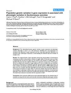
Figure 1: Spread from the frontier of a population (A) and, later, by remotely dispersed individuals (B) that yield an asymptotically infinite velocity for a deterministic nonlinear model (Kot et al. 1996) but a finite furthest-forward velocity for a nonlinear stochastic process. Here, we propose a method, based on invasion by "extreme events," that corresponds to changes in the location of the furthest-forward individual. The example that follows this background theory uses dispersal kernels fitted to seed rain data that are both fat-tailed and possess infinite variance. Spread by Extreme Dispersal The difference between theoretical moments of distributions and those of data result in qualitatively different predictions of population spread. Exponentially bounded kernels can behave like the data used to fit them (Clark et al. 2001): they.liave all moments finite, and, when embedded in population models, they predict a traveling wave of advance. Fat-tailed kernels and kernels for which some moments do not exist may not behave like the data fitted to those kernels, in the sense that the data have empirical moment-generating functions and finite moments, whereas the fitted kernel does not. This section provides a means for estimating the velocity of spread that results from dispersal patterns that are best fitted by fat-tailed kernels that may possess few finite moments (as few as one). We define the net reproductive rate, R^, as the number of offspring that can be expected from an individual at the time of seed release. It can sometimes be convenient to define R^ as the number of offspring expected following some (density-independent) mortality of juveniles. This is
simply a matter of bookkeeping. Because dispersal is typically estimated from seed (rather than seedlings or saplings), our definition of JRo based on seed is most readily applied to dispersal data. Our model assumes linear population growth up to some finite maximum density, and thus is comparable to traditional (diffusion, integrodifferential, and integrodifference) models of spread. Our application of the model is cognizant of the fact that migrations usually take place in the presence of other species. Our estimates of R,, are based on field estimates of fecundity and survivorship in a competitive environment. #o can be much greater than 1 during an initial advance, as the population increases from low density. Thus, the model has broad relevance to invasion problems, and the specific application here accommodates the measured effects of mortality in actual stands of trees. Consider a parent that produces an average of £„ offspring over its lifetime with dispersal described by kernel j[x). If the kernel is sufficiently fat-tailed, and the net reproductive rate, R,,, is sufficiently large, the population can spread as a series of remote subpopulations established by extremely placed offspring (Davis 1987; Lewis 1997; Shigesada and Kawasaki 1997; fig. 15). The distribution of leaps forward might be approximated by the sum of random variates drawn from the distribution of furthestdispersing propagules, that is, extremes. With a fat tail, there is a good chance that the extremely placed individual will find itself distant from the population frontier or even from the next closest disperser. This dislocation means that the extremely placed individual becomes the basis for additional spread. Unlike a diffusing population, the expanding "front" is not supported by a large, nearby pop-
540
The American Naturalist
0^.200 150
DWanca(m)
Figure 2: The relationship between the dispersal kernel fix) (dashed line, eq. [10]) and the density of extreme dispersers f(x, 1) for three different net reproductive rates: R» = 2 (/I), £„ = 20 (B), £,, = 200 (Q. The vertical dashed line marks the expected extreme disperser (eq. [12]). illation (e.g., a traveling wave). To estimate spread, we can avoid the complexity of previous approaches by concentrating on the extremes. Here, we derive this distribution of extreme dispersal for a parametric kernel as basis for estimating rate of spread. Let p(x; N)dx be the probability that the furthestdispersing individual from a group of N evenly spaced parents settles on the interval [x, x+ dx}. The probability density function (PDF) for a seed that arises from a single parent is the product of the events that a seed settles at x and all other seeds from the parent settle closer to the source:
p(x; 1) = Raf(x)\
f(y}dy
- co < x < co,
(1)
where f(x) is the dispersal kernel (also a PDF). The factor J?o in equation (1) is the number of ways in which we can obtain a given outcome (any one of ^ total offspring can be the extreme case). The "1" in p(x; 1) refers to extreme dispersal from a single parent plant to distinguish this distribution from one derived for the edge of a continuous population (see below). We arrive at the same density starting from the probability that the extreme disperser lies to the left of a point located distance x to the right of the parent, that is, the cumulative distribution function (CDF):
f(y)dy
= [*{*)]*
(2)
where F(x) is the CDF for the dispersal kernel f(x]. Differentiation yields the PDF for the furthest-forward disperser:
p(x; 1) =
(3)
which is equivalent to equation (1). The development of equations (l)-(3) can be viewed as an application of order statistics, with P(x, 1) being the sampling distribution of the .Rjth quantile (e.g., Stuart and Ord 1994). The density of extremes incorporates the contributions of both the dispersal kernel and the net reproductive rate, RQ (fig. 2). Net reproductive rate has a dramatic effect on the extremes. With £0 = 2, extreme dispersal does not much exceed the kernel itself (fig. 2A). With R0 = 200, the extremes extend well beyond the dispersal kernel (fig. 2Q. Extremes Derived from the Continuous Population Upper and lower bounds on population spread per generation, c, can be derived under differing assumptions on distribution of the parent population. Spread by leaps from one extremely placed colony to the next (fig. IB) approx-
Dispersal and Population Spread imates migration far from a population center. A lower bound c~ comes from assuming that the only possible parent for the furthest-forward individual is the furthestforward individual from the last generation. Initially, spread could commence from the edge of a continuous population, supported by the large nearby seed source (fig. 1A); fat-tailed dispersal subsequently shifts the process to spread by extremes (fig. 15). As discussed below, an upper bound c+ comes from assuming that the possible parents for the furthest-forward individual occupy a closed stand at density llh (fig. 1A) for crown size h. Abundant seed means that the initial spread from a continuous population can be more rapid than the rate that prevails later, when spread is perpetuated by scattered individuals. If we assume that spread commences from the edge of a continuous population (fig. 1A), and that fat-tailed dispersal subsequently shifts the process to spread by extremes (fig. IB), then c+ and c~ suggest initial and asymptotic spread rates for the population. This interpretation in terms of initial and final spread rates is not proved mathematically. Here, we derive the initial spread depicted in figure 1A. As shown below, our estimates for "initial" rates and "eventual" rates give upper and lower bounds for population spread rate. Consider a transect perpendicular to a population frontier, where seed source is distributed more or less evenly to the left of the front at x = 0 (fig. 1A). The population spreads to the right at an initial rate determined by offspring that can originate from parents located anywhere to the left of x = 0 (i.e., x< 0). Density dependence is implicit because the continuous population is constrained to have an upper limit on seed production (and canopy coverage) at density llh. The parameter h can be viewed as the distance between individual trees, and Nh is the linear extent (width) of the population. Seed production is distributed at locations along the transect (~xNh, ...,-Xj,0). Assuming that individuals each produce R^ offspring, the probability that the extreme disperser travels no further to the right than x is the CDF
P(x;N) =
Note that equation (2) is the special case where N = 1. The corresponding PDF is
(4)
where
pt(x; N) =
541
R0f(x + xhk)P(x-> N) F(x + xhk)
Here, each pk(x; N) is associated with the event that the individual at location — hk produces the extreme offspring. To see this more clearly, observe that x JAT) r c + x 11S°~' n 1), the vast majority of individuals may contribute no offspring to the next generation. Examples include most plants (Clark et al. 1998«), birds (Lande 1987), and sea turtles (Grouse et al. 1987). Thus, ^ represents an average over a large number of zeros and a small minority that do indeed produce^ offspring. The zeros are those individuals censused at seed or seedling stages that do not survive to reproductive age. Here, we recast the standard lifehistory equation to accommodate this reproductive variability among individuals, and we propagate that variability to the density of dispersal distances. In other words, we translate reproductive variability into variability in spread. To insure that we do not exaggerate the impact, we use a highly conservative estimate of variance. We include only the variance implicit to the standard life-history equation itself, that is, that which results from variable life span described by the survivor function. In practice, there will be many more sources of variance in R, o•* . o C d 3 OJ . it o d
C) I | I,
o G3 0
100
200 300 Rate(m/yr)
400
500
Results The^Effect of Extreme Dispersal Our approach predicts a pattern of spread that might be viewed as a hybrid of previous methods. The example using parameter values for Acer rubrum shows a constant average rate (fig. 5A, SB), as occurs with simple diffusion models. The pattern differs from diffusion in that spread proceeds as a series of irregular leaps (fig. 55). These most extreme dispersers are peak values in figure SB and represent the formation of distant centers for additional spread. Although the long-term rate of spread approaches a constant expectation, which is predicted by equation (12) (dashed line, fig. SB, 5Q, that rate is much greater than would occur by diffusion. The mean spread rate of 40 m yr~' in figure 5 contrasts with 10 and 20 m yr~' predicted by Gaussian and exponential dispersal kernels, respectively,
Figure 5: Simulated spread from extreme dispersal for Acer rubrum. A, Cumulative distance traveled over successive generations for 10 simulations. B, Distances traveled by generation for the 10 simulations in A. C, Comparison of distribution of extreme dispersal events from B (shaded bars) and the long-term (100 generations) distribution of rates g(c) (step curve). The dashed line in B and Cis the expectation from equation (12). The distribution of extreme events is skewed, as predicted by equations (1) and (11). The distribution of rates approaches normality with increasing numbers of generations. The distribution of rates has a mean of 45.4 ± 7.70 m yr"1 with 95% of values on the interval (36.1, 64.2). Units in C (m yr~') are obtained by scaling for generation time (eq. [6]). fitted to the same data. Whereas the fitted kernel used to simulate spread in figure 5 has infinite variance, the simulations provide a finite variance for a distribution of rates that is asymptotically normal (fig. 5C). This distribution
546 The American Naturalist corresponds to g(c;l) in equation (5). Moreover, the average rate of spread from simulation agrees with the mean of the distribution of extremes; the estimate from equation (11) is shown as a dashed line in figure 5B and 5C. We prove this rate to be finite for all relevant assumptions, in the appendix. Although net reproductive rate has a minor effect on the rate of diffusion (for a Gaussian kernel, the rate is proportional to the square root of the log of £,,), the density of extremes captures its dominant effect on fat-tailed spread. For a species with low R,, and short dispersal distances, such as Carya, the most extremely placed seed only reaches 5-50 m (fig. 6A). By contrast, wind-dispersed types produce many small seeds, and the extreme disperser might travel 102-104 m (fig. 6B). In the case of Betula, the
extreme disperser is predicted to always exceed 500 m. The densities of extreme dispersal (fig. 6) predict rates of spread that range over two orders of magnitude (fig. 7). Winddispersed types (Betula, Acer, Liriodendrori) have highest rates (30-80 m yr~'); animal-dispersed types (Cornus, Nyssa, Carya) have low rates (0.1-1 m yr"1). depending on N. The Effect of Variable Reproduction Variable reproduction slows rates of spread using our parameterizations for tree populations. Figure 8A shows a typical density (A. rubrum) of net reproductive rates. The density is represented on a log-log plot because the tail would otherwise be obscure. The assumption that 1 in
A)
B)
(D o , d to q . d
Carya Cornus Nyssa Quercus
s d
Acer Betula Fraxlnus Liriodendron Pinus Tilia
m 8 j o
CVl q d
p d o d
50
100
150
200
500
1000
1500
2000
Distance (m) Figure 6: Densities of extreme dispersers for animal-dispersed (A) and wind-dispersed (B) types from equation (11). Note different scales for horizontal axes.
Dispersal and Population Spread
o o Betula
I
I
Acer
Liriodendron
densities assume the same mean R^, variation of the type caused by high juvenile mortality slows the rate of spread. For juvenile survivorship of 0.001, variable R,, profoundly limits the rate of spread estimated from our dispersal data. We found that invasion progressed two orders of magnitude slower for variable R,, than it did for constant RQ (fig. 95). Poorly dispersed species are predicted to spread on the order of meters per century. Increasing the rate of spread requires much higher juvenile survivorship (S(f,) in eq. [14]), which results, in turn, in higher RQ.
* Tilia Fraxinus
Application to Contemporary Spread
£ 8 ^
There are few examples of contemporary tree invasions for which estimates of life history, dispersal, and invasion rates are available. Dispersal estimates and invasion rates for two spruce (Picea) species in Alaska allow for model application. We combined dispersal estimates obtained from a remnant white spruce stand into a surrounding clearcut with rates of Sitka spruce spread into Glacier Bay.
Pinus
O TC)
! j Carya
I
547
Nyssa
Cornus
A) Distribution of net reproductive rate
q ci
CO 0.05
0.10
0.50
ln(H0)/7
Figure 7: The ranges of spread rates plotted against rates of increase In (R,)IT estimated from dispersal and life-history data for southern Appalachian trees. A range is given for each taxon that has upper and lower bounds that are numerical estimates. The interior tick mark is the analytical result from equation (12).
1,000 seeds reach.,reproductive age is within the range we observe in modern forests (Clark et al. 1998). This high juvenile mortality is represented by the bulk of the density (99.9%) at the low extreme of figure 8A. The remaining tail contains 0.001 (the probability of at least some reproduction). The two densities of extreme dispersal in figure 8B demonstrate the effect of variable recruitment. The upper curve is the density that results from a constant R,, (eq. [11]). The lower curve is the density that accommodates variance in RQ (eq. [7]). This density is lower than that for constant .Ro because it includes a large zero class corresponding to the bulk of the R^ values that equal zero (for clarity, this zero class is not shown). The large zero class means that the overall expectation of extreme dispersal is much lower than predicted for a constant RQ. Thus, although both
ta
§0-^
E CO -3 3
-3 Analytical solution
0 3 Simulation, variable RO
Figure 9: Comparisons of spread rates. A, Simulation results (vertical axis) agree with the analytical model (horizontal axis) summarized by the mean (eq. [12]). B, Rates of spread that include the full density of R, values from equation (7) (horizontal axis) are consistently lower than are those that assume the mean R, (eq. [6]). Both axes are log values. Fastie (1995) found that the rate of spread into deglaciated the lower estimate of c~, and some seed might travel from terrain depended on distance to the closest seed source, distant, continuous stands. with rates averaging from 300 to 400 m yr~'. To estimate a dispersal kernel, we used seed trap data from transects Discussion emanating from the remnant stand (S. Rupp, unpublished manuscript). Our maximum likelihood approach assumes Spread predictions that ignore variance contain order of a seed source that is everywhere constant within the stand, magnitude bias. Our solution to the problem of spread and seeds are dispersed in all directions according to a that results from fat-tailed dispersal provides two new in2Dt kernel (Clark et al. 1999). The mean of the Poisson sights that depart from former views. First, we demonstrate sampling distribution is given by the 2Dt kernel integrated that spread is intermediate in character and in rate between over the source area. Dispersal parameters from nine tran- simple diffusion and fat-tailed dispersal predicted by presects averaged u = 5,531 ± 3,024 m2. Because we lack full vious models. Second, we show that reproductive varialife-history data, we considered the range of R$ values bility can have a profound effect on the rate of spread. (5,000-50,000) we obtain for tree species having winddispersed seed and having fecundity rates similar to those Dispersal Is Discrete estimated here (Clark 1998). The geometric mean value for this range is 16,000. We further assume T = 50 yr Previous results showed that velocities predicted from (Fastie 1995), the maximum likelihood estimates for u mean dispersal distances (i.e., diffusion) are qualitatively from our nine transects, no covariance in u and RQ, and and quantitatively inaccurate (Mollison 1972; Kot et al. a standard error on RQ of 1,000. We bootstrapped spread 1996; Lewis 1997; Clark 1998), but analyses from fat-tailed rates using equation (12). The bootstrap is thus parametric kernels produce no asymptotic estimate; spread just accelerates indefinitely (Kot et al. 1996). By acknowledging in RQ and nonparametric in u. The distribution of bootstrapped estimates straddles that individuals are discrete, we obtain estimates of spread Fastie's (1995) estimate based on stand reconstruction (fig. that are faster and noisier than diffusion but still finite 10). The skewed pattern of spread rates results from a (fig. 5). Our simulation method that uses the same "sample limited number of u parameter estimates with uncertainty size" as a parent (i.e., J^) allows calculations of means, resulting from a limited number of sample years. The variances, and so forth. The analytical calculation for the broad range of estimates is consistent with the prediction mean agrees with simulation (fig. 9A). The simple apof highly variable rates, yet the central tendency is close proximation represented by equation (12) provides a rule to the observed rate. Our data underestimate the rate of of thumb that can be readily estimated from a fitted kernel. spread, but we expected an underestimate because we used The approach can be implemented in the common situ-
Dispersal and Population Spread
Bootstrapped estimates
aoo
1000
400 600 C" estimates (myr1)
Fitted kernel and extremes
a) O
549
Any invasion by leptokurtic dispersal is sensitive to the shape of the tail (Kot et al. 1996; Clark 1998). Because the tail cannot be adequately characterized, assuming a parametric, fat-tailed kernel makes for speculative interpretation. However, unlike traditional models, our solution does not "blow up." Our method is much less susceptible to errors in the tail because a random sample of size R^ from a kernel fitted to data produces a simulated data set much like the original data (fig. 4). The infinite tail that controls the predictions of parametric models does not contribute to the discrete samples drawn from such densities. By acknowledging that propagules are discrete, we avoid the extreme sensitivity to tail shape that makes traditional models unsatisfactory. The effect of R 0 and
Hence, if £[X=] < oo, then £[17,] < oo. Second, there is a constant c = c(F] such that
E[X+ | R] Thus, if £[77,] < oo, and E[R] < oo, then £[X+] < oo. (Note: If N is a random variable, then E[N] < oo, E[R] < oo, and •Efail < °°> implying that E[X+] < oo.) Literature Cited
multiple pathways of primary succession at Glacier Bay, Alaska. Ecology 76:1899-1916. Andow, D. A., P. M. Kareiva, S. Levin, and A. Okubo. Johnson, W. C., and T. Webb III. 1989. The role of blue jays in the postglacial dispersal of fagaceous trees in 1990. Spread of invading organisms. Landscape Ecology eastern North America. Journal of Biogeography 16: 4:177-188. 561-571. Bennett, K. D. 1987. Holocene history of forest trees in Kot, M., M. A. Lewis, and P. van den Driessche. 1996. southern Ontario. Canadian Journal of Botany 65: Dispersal data and the spread of invading organisms. 1792-1801. Ecology 77:2027-2042. . 1998. Why trees migrate so fast: confronting theory with dispersal biology and the paleorecord. Amer- Lande, R. 1987. Extinction thresholds in demographic models of territorial populations. American Naturalist ican Naturalist 152:204-224. 130:624-635. Clark, J. S., C. Fastie, G. Hurtt, S. T. Jackson, C. Johnson, G. King, M. Lewis, et al. 1998a. Reid's paradox of rapid Larcher, W., and H. Bauer. 1981. Ecological significance of resistance to low temperature. Pages 403-437 in O. plant migration. BioScience 48:13-24. L. Lange, P. S. Nobel, C. B. Osmond, H. Ziegler, eds. Clark, J. S., E. Macklin, and L. Wood. 1998&. Stages and Encyclopedia of plant physiology. Springer, Berlin. spatial scales of recruitment limitation in southern Appalachian forests. Ecological Monographs 68:213-235. Lewis, M. A. 1997. Variability, patchiness and jump dispersal in the spread of an invading population. In D. Clark, J. S., M. Silman, R. Kern, E. Macklin, and J. Tilman and P. Kareiva, eds. Spatial ecology. Princeton HilleRisLambers. 1999. Seed dispersal near and far: gen-*University Press, Princeton, N.J. eralized patterns across temperate and tropical forests. Lubina, J. A., and S. A. Levin. 1988. The spread of a reEcology 80:1475-1494. invading species: range expansion in the California-sea Clark, J. S., L. Hprvath, and M. Lewis. 2001. On the esotter. American Naturalist 131:526-543. timation of spread for a biological population. Statistics Mollison, D. 1972. The rate of spatial propagation of simand Probability Letters 51:225-234. ple epidemics. Proceedings of the sixth Berkeley SymGrouse, D., L. Crowder, and H. Caswell. 1987. A stageposium on Mathematics, Statistics, and Probability 3: based model for loggerhead sea turtles and implications 579-614. for conservation. Ecology 68:1412-1423. . 1977. Spatial contact models for ecological and Davis, M. B. 1981. Quaternary history and the stability of epidemic spread. Journal of the Royal Statistical Society forest communities. Pages 132-153 in D. C. West, H. B 39:283-326. H. Shugart, and D. B. Botkin, eds. Forest succession: Portnoy, S., and M. F. Willson. 1993. Seed dispersal curves: concepts and application. Springer, New York. behavior of the tail of the distribution. Evolutionary . 1987. Invasion of forest communities during the Biology 7:25-44. Holocene: beech and hemlock in the Great Lakes region. Pages 373-393 in A. J. Gray, M. J. Crawley, and P. J. Sakai, A., and C. J. Weiser. 1973. Freezing resistance of Edwards, eds. Colonization, succession, and stability. trees in North America with reference to tree regions. Blackwell Scientific, Oxford. Ecology 54:118-126. Fastie, C. L. 1995. Causes and ecosystem consequences of Shigesada, N., and K. Kawasaki. 1997. Biologicial inva-
554 The American Naturalist sions: theory and practice. Oxford Series in Ecology and Evolution. Oxford University Press, Oxford. Skellam, J. G. 1951. Random dispersal in theoretical populations. Biometrika 38:196-218. Stuart, A., and J. K. Ord. 1994. Kendall's advanced theory of statistics. Arnold, London. Taylor, R. A. 1978. The relationship between density and distance of dispersing insects. Ecological Entomology 3: 63-70. Turchin, P. 1998. Quantitative analysis of movement. Sinauer, Sunderland, Mass. Van den Bosch, E, J. A. J. Metz, and O. Diekmann. 1990. The velocity of spatial population expansion. Journal of Mathematical Biology 28:529-565.
Weinberger, H. F. 1982. Long-time behavior of a class of biological models. SLAM (Society for Industrial and Applied Mathematics) Journal of Mathematical Analysis 13:353-396. Wright, H. E., Jr. 1992. Patterns of Holocene climatic change in the midwestern United States. Quaternary Research 38:129-134. Wyckoff, P. H., and J. S. Clark. 2000. Predicting tree mortality from diameter growth: a comparison of maximum likelihood and Bayesian approaches. Canadian Journal of Forest Research 30:156-167. Associate Editor: Lewi Stone