Porcellio scaber algorithm (PSA) for solving constrained optimization ...

Porcellio scaber algorithm (PSA) for solving constrained optimization problems Yinyan Zhang1 ,⋆ , Shuai Li1 ,⋆⋆ , and Hongliang Guo2 ,⋆⋆⋆

arXiv:1710.04036v1 [cs.NE] 11 Oct 2017

1

Department of Computing, The Hong Kong Polytechnic University, Hong Kong, China Center for Robotics, School of Automation Engineering, University of Electronic Science and Technology of China, Chengdu, China

2

Abstract. In this paper, we extend a bio-inspired algorithm called the porcellio scaber algorithm (PSA) to solve constrained optimization problems, including a constrained mixed discrete-continuous nonlinear optimization problem. Our extensive experiment results based on benchmark optimization problems show that the PSA has a better performance than many existing methods or algorithms. The results indicate that the PSA is a promising algorithm for constrained optimization.

1 Introduction Modern optimization algorithms may be roughly classified into deterministic optimization algorithms and stochastic ones. The former is theoretically sound for well-posed problems but not efficient for complicated problems. For example, when it comes to nonconvex or large-scale optimization problems, deterministic algorithms may not be a good tool to obtain a globally optimal solution within a reasonable time due to the high complexity of the problem. Meanwhile, while stochastic ones may not have a strong theoretical basis, they are efficient in engineering applications and have become popular in recent years due to their capability of efficiently solving complex optimization problems, including NP-hard problems such as the travelling salesman problem. Bio-inspired algorithms take an important role in stochastic algorithms for optimization. These algorithms are designed based on the observations of animal behaviors. For example, one of the well known bio-inspired algorithm called particle swarm optimization initially proposed by Kennedy and Eberhart [1] is inspired by the social foraging behavior of some animals such as the flocking behavior of birds. There are some widely used benchmark problems in the field of stochastic optimization. The pressure vessel design optimization problem is an important benchmark problem in structural engineering optimization [2]. The problem is a constrained mixed discrete-continuous nonlinear optimization problem. In recent years, many bioinspired algorithms have been proposed to solve the problem [3–6]. The widely used benchmark problems also include a nonlinear optimization problem proposed by Himmelblau [7]. ⋆ e-mail: [email protected] ⋆⋆ e-mail: [email protected] ⋆⋆⋆ e-mail: [email protected]

Recently, a novel bio-inspired algorithm called the porcellio scaber algorithm (PSA) has been proposed by Zhang and Li [8], which is inspired by two behaviors of porcellio scaber. In this paper, we extend the result in [8] to solve constrained optimization problems. As the original algorithm proposed in [8] deals with the case without constraints, we provide some improvements for the original PSA so as to make it capable of solving constrained optimization problems. Then, we compare the corresponding experiment results with reported ones for the aforementioned benchmark problems as case studies. Our extensive experiment results show that the PSA has much better performance in solving optimization problems than many existing algorithms. Before ending this introductory section, the main contributions of this paper are listed as follows: 1)We extend the PSA to solve constrained optimization problems, including the constrained mixed discretecontinuous nonlinear optimization problem. 2)We show that the PSA is better than many other existing algorithms in solving constrained optimization problems by extensive numerical experiments.

2 Problem Formulation The constrained optimization problem (COP) considered in this paper is presented as follows: minimize fˇ(x), subject to g j (x) ≤ 0, li ≤ xi ≤ ui ,

(1)

with i = 1, 2, · · · , d and j = 1, 2, · · · , m, where x = [x1 , x2 , · · · , xd ]T is a d-dimension decision vector; li and ui are the corresponding lower bound and upper bound of the ith decision variable; fˇ(x) : Rd → R is the cost function

Algorithm 1 Original PSA Cost function f (x), x = [x1 , x2 , · · · , xd ]T Generate initial position of porcellio scaber x0i (i = 1, 2, · · · , N) Environment condition Ex at position x is determined by f (x) Set weighted parameter λ for decision based on aggregation and the propensity to explore novel environments Initialize f∗ to an extremely large value Initialize each element of vector x∗ ∈ Rd to an arbitrary value while k < MaxS tep do Get the position with the best environment condition, i.e., xb = arg minxkj { f (xkj )} at the current time among the group of porcellio scaber if minxkj { f (xkj )} < f∗ then x∗ = xb f∗ = minxkj { f (xkj )} end if Randomly chose a direction τ = [τ1 , τ2 , · · · , τd ]T to detect Detect the best environment condition min{Ex } and worst environment condition max{Ex } at position xki + τ for i = 1 : N all N porcellio scaber for i = 1 : N all N porcellio scaber do Determine the difference with respect to the position to aggregate i.e., xki − arg minxkj { f (xkj )}) Determine where to explore, i.e., pτ Move to a new position according to (2) end for end while Output x∗ and the corresponding function value f∗ Visualization

to be minimized. For the case that the problem is convex, there are many standard algorithms to solve the problem. However, for the case that the problem is not convex, the problem is difficult to solve.

3 Algorithm Design

where λ ∈ (0, 1), τ is a vector with each element being a random number, and p is defined as follows: p=

f (xki + τ) − min{ f (xki + τ)} max{ f (xki + τ)} − min{ f (xki + τ)}

Evidently, the original PSA does not take constraints into consideration. Thus, it cannot be directly used to solve COPs. 3.2 Inequality constraint conversion

In this subsection, we provide some improvements for the original PSA and make it capable of solving COPs. As the original PSA focuses on solving unconstrained problem, we first incorporate the inequality constraints g j (x) ≤ 0 ( j = 1, 2, · · · , m) into the cost function. To this end, the penalty method is used, and a new cost function is obtained as follows: fˇ(x) = f (x) + γ

m X

g2i (x)h(gi(x)),

3.1 Original PSA

For the sake of understanding, the original PSA is given in algorithm 1 [8], which aims at solving unconstrained optimization problems of the following form: minimize f (x), where x is the decision vector and f is the cost function to be minimized. The main formula of the original PSA is given as follows [8]: xik+1 = xki − (1 − λ)(xki − arg min{ f (xkj )}) + λpτ, xkj

(2)

(3)

i=1

where h(gi (x)) is defined as    1, if gi (x) > 0, h(gi (x)) =   0, if gi (x) ≤ 0, and γ ≫ 1 is the penalty parameter. By using a large enough value of γ (e.g., 1012 ), unless all the inequality constraints gi (x) ≤ 0 (i = 1, 2, · · · , m) are satisfied, PN 2 the term γ i=1 gi (x)h(gi(x)) takes a dominant role in the cost function. On the other hand, when all the inequality constraints gi (x) ≤ 0 (i = 1, 2, · · · , m) are satisfied, h(gi (x)) = 0, ∀i, and thus fˇ(x) = f (x). 3.3 Addressing simple bounds

In terms of the simple bounds l j ≤ x j ≤ u j with j = 1, 2, · · · , d, they are handled via two methods. Firstly, to satisfy the simple bounds, the initial position of each porcellio scaber is set via the following formula: x0i, j = l j + (u j − l j ) × rand(0, 1)

In this section, we modify the original PSA [8] and provide an improved PSA for solving COPs.

.

(4)

where x0i, j denotes the initial value of the jth variable of the position vector of the ith (with i = 1, 2, · · · , N) porcellio scaber; rand(0, 1) denotes a random number in the region (0, 1), which can be realized by using the rand function in Matlab. The formula (4) guarantees that the initial positions of all the porcellio scaber satisfy the the simple bounds l j ≤ x j ≤ u j with j = 1, 2, · · · , d. Secondly, if the positions of all the porcellio scaber are updated according to (2) by replacing f (x) with fˇ(x) defined in (3) for the constrained optimization problem (1), then the updated values of the position vector xki may violate the simple bound constraints. To handle this issue, based on (2), a modified evolution rule is proposed as follows: xik+1 = PΩ (xki − (1 − λ)(xki − arg min{ fˇ(xkj )}) − λpτ), (5) xkj

Algorithm 2 Algorithm for the evaluation of PΩ (x) with x = [x1 , x2 , · · · , xd ]T for i = 1 : d do if x1 < li then xi = li end if if xi > ui then xi = u i end if end for return y = [x1 , x2 , · · · , xd ]T

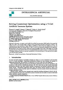
Figure 1. A diagram showing the design parameters of a pressure vessel [9].

where λ ∈ (0, 1), τ is a vector with each element being a random number, and p=

fˇ(xki + τ) − min{ fˇ(xki + τ)} . max{ fˇ(xk + τ)} − min{ fˇ(xk + τ)} i

i

Besides, PΩ is a projection function and make the updated position satisfy the simple bound constraints, where Ω = {x ∈ Rd |li ≤ xi ≤ ui , i = 1, 2 · · · , d}. The mathematical definition of PΩ (x) is PΩ (x) = arg miny∈Ω ky − xk2 with k · k2 denoting the Euclidean norm. The algorithm for the evaluation of PΩ (x) is given in Algorithm 2.

Algorithm 3 PSA for COPs Cost function fˇ(x) as defined in (3), x = [x1 , x2 , · · · , xd ]T Generate initial position of porcellio scaber x0i (i = 1, 2, · · · , N) according to (4) Environment condition Ex at position x is determined by fˇ(x) Set weighted parameter λ for decision based on aggregation and the propensity to explore novel environments Set penalty parameter γ in fˇ(x) to a large enough value Initialize f∗ to an extremely large value Initialize each element of vector x∗ ∈ Rd to an arbitrary value while k < MaxS tep do Get the position with the best environment condition, i.e., xb = arg minxkj { f (xkj )} at the current time among the group of porcellio scaber if minxkj { f (xkj )} < f∗ then x∗ = xb f∗ = minxkj { f (xkj )} end if Randomly chose a direction τ = [τ1 , τ2 , · · · , τd ]T to detect Detect the best environment condition min{Ex } and worst environment condition max{Ex } at position xki + τ for i = 1 : N all N porcellio scaber for i = 1 : N all N porcellio scaber do Determine the difference with respect to the position to aggregate i.e., xki − arg minxkj { f (xkj )}) Determine where to explore, i.e., pτ Move to a new position according to (5) where PΩ (x) is evaluated via Algorithm 2 end for end while Output x∗ and the corresponding function value f∗ Visualization

3.4 PSA for COPs

Based on the above modifications, the resultant PSA for solving COPs is given in Algorithm 3. In the following section, we will use some benchmark problems to test the performance of the PSA in solving COPs.

4 Case Studies In this section, we present experiment results regarding using the PSA for solving COPs. 4.1 Case I: Pressure vessel problem

In this subsection, the pressure vessel problem is considered. The pressure vessel problem is to find a set of four design parameters, which are demonstrated in Fig. 1, to minimize the total cost of a pressure vessel considering the cost of material, forming and welding [1]. The four design parameters are the inner radius R, and the length

L of the cylindrical section, the thickness T h of the head, the thickness T s of the body. Note that, T s and T h are integer multiples of 0.0625 in., and R and L are continuous variables.

Table 1. Comparisons of best results for the pressure vessel problem

[4] [9] [3] [10] [11] [12] [13] [14] [15] [16] [17] [18] [19] [20] PSA

x1

x2

x3

x4

g1 (x)

g2 (x)

g3 (x)

g4 (x)

f (x)

0.8125 0.7782 0.8125 1.125 1.125 1.125 0.8125 0.9375 1.125 0.8125 1.000 0.8125 1 0.8125 0.8125

0.4375 0.3846 0.4375 0.625 0.625 0.625 0.4375 0.5000 0.625 0.4375 0.625 0.4375 0.625 0.4375 0.4375

42.0984 40.3196 42.0984 58.2789 48.97 58.1978 40.3239 48.3290 58.291 41.9768 51.000 42.0870 51.2519 42.0984 42.0952

176.6366 200.000 176.6366 43.7549 106.72 44.2930 200.0000 112.6790 43.690 182.2845 91.000 176.7791 90.9913 176.6378 176.8095

8.00e-11† -3.172e-5 8.00e-11† -0.0002 -0.1799 -0.00178 -0.034324 -0.0048 0.000016 -0.0023 -0.0157 -2.210e-4 -1.011 -8.8000e-7 -6.2625e-5

-0.0359 4.8984e-5† -0.0359 -0.06902 -0.1578 -0.06979 -0.05285 -0.0389 -0.0689 -0.0370 -0.1385 -0.03599 -0.136 -0.0359 -0.0359

-2.724e-4 1.3312† -2.724e-4 -3.71629 97.760 -974.3 -27.10585 -3652.877 -21.2201 -22888.07 -3233.916 -3.51084 -18759.75 -3.5586 -738.7348

-63.3634 -40 -63.3634 -196.245 -132.28 -195.707 -40.0000 -127.3210 -196.3100 -57.7155 -149 -63.2208 -149.009 -63.3622 -63.1905

6059.7143 5885.33 6059.7143 7198.433 7980.894 7207.494 6288.7445 6410.3811 7198.0428 6171.000 7079.037 6061.1229 7172.300 6059.7258 6063.2118

† means that the corresponding constraint is violated. Algorithm 4 Algorithm for PΩ (x = [x1 , x2 , x3 , x4 ]T ) in the pressure vessel problem y1 = round(x1 /0.0625) × 0.0625 if y1 < 0.0625 then y1 = 0.0625 end if if y1 > 99 × 0.0625 then y1 = 99 × 0.0625 end if y2 = round(x2 /0.0625) × 0.0625 if y2 < 0.0625 then y2 = 0.0625 end if if y2 > 99 × 0.0625 then y2 = 99 × 0.0625 end if if x3 < 10 then y3 = 10 end if if x3 > 200 then y3 = 200 end if if x4 < 10 then y4 = 10 end if if x4 > 200 then y4 = 200 end if return y = [y1 , y2 , y3 , y4 ]T Let x = [x1 , x2 , x3 , x4 ]T = [T s , T h , R, L]T . The pressure vessel problem can be formulated as follows [9]: minimize f (x) = 0.6224x1 x3 x4 + 1.7781x2 x23 + 3.1661x21 x4 + 19.84x21 x3 , subject to g1 (x) = −x1 + 0.0193x3 ≤ 0, g2 (x) = −x2 + 0.00954x3 ≤ 0, 4 g3 (x) = −πx23 x4 − πx33 + 1296000 ≤ 0, 3 g4 (x) = x4 − 240 ≤ 0,

Evidently, this problem has a nonlinear cost function, three linear and one nonlinear inequality constraints. Besides, there are two discrete and two continuous design variables. Thus, the problem is relatively complicated. As this problem is a mixed discrete-continuous optimization, the projection function PΩ (x) is slightly modified and presented in Algorithm 4. Besides, the initialization of the initial positions of porcellio scaber is modified as follows: x0i,1 = 0.0625 + f loor((99 − 1) × rand) × 0.0625, x0i,2 = 0.0625 + f loor((99 − 1) × rand) × 0.0625, x0i,3 = 10 + f loor(200 − 10) × rand, x0i,4 = 10 + f loor(200 − 10) × rand, where x0i, j denotes the jth variable of the position vector of the ith porcellio scaber; f loor(y) = argminx∈{0,1,2,··· } {x + 1 > y}, i.e., the f loor function obtains the integer part of a real number; rand denotes a random number in the region (0, 1). The functions f loor and rand are available at Matlab. The best result we obtained using the PSA in 1000 instances of executions and those by using various existing algorithms or methods for solving this problem are listed in Table 1. Note that, in the experiments, 40 porcellio scaber are used, the parameter λ is set to 0.6, and the MaxS tep is set to 100000 with τ being a zero-mean random number with the standard deviation being 0.1. As seen from Table 1, the best result obtained by using the PSA is better than most of the existing results. Besides, the difference between the best function value among all the ones in the table and the best function value obtained via using the PSA is quite small. 4.2 Case II: Himmelblau’s nonlinear optimization problem

In this subsection, we consider a nonlinear optimization problem proposed by Himmelblau [7]. This problem is

Table 2. Comparisons of best results for Himmelblau’s nonlinear optimization problem

[21] [22] [23] [7] [24] PSA

x1

x2

x3

x4

x5

g1 (x)

g2 (x)

g3 (x)

f (x)

78.0 78.00 81.4900 78.6200 78.00 79.9377

33.0 33.00 34.0900 33.4400 33.00 33.8881

27.07997 29.995 31.2400 31.0700 29.995256 28.5029

45.0 45.00 42.2000 44.1800 45.00 41.3052

44.9692 36.776 34.3700 35.2200 36.775813 41.7704

92.0000 90.7147 90.5225 90.5208 92 91.6157

100.4048 98.8405 99.3188 98.8929 98.8405 100.4943

20.0000 19.9999† 20.0604 20.1316 20 20.0055

-31025.5602 -30665.6088 -30183.576 -30373.949 -30665.54 -30667.8113

† means that the corresponding constraint is violated. also one of the well known benchmark problems for bioinspired algorithms. The problem is formally described as follows [7]: minimize f (x) =5.3578547x23 + 0.8356891x1 x5 + 37.29329x1 − 40792.141, subject to g1 (x) =85.334407 + 0.0056858x2 x5 + 0.00026x1 x4 − 0.0022053x3 x5 , g2 (x) =80.51249 + 0.0071317x2 x5 + 0.0029955x1 x2 + 0.0021813x23, g3 (x) =9.300961 + 0.0047026x3 x5 + 0.0012547x1 x3 + 0.0019085x3 x4 , 0 ≤ g1 (x) ≤ 92, 90 ≤ g2 (x) ≤ 110, 20 ≤ g3 (x) ≤ 25, 78 ≤ x1 ≤ 102, 33 ≤ x2 ≤ 45, 27 ≤ x3 ≤ 45, 27 ≤ x4 ≤ 45, 27 ≤ x5 ≤ 45, with x = [x1 , x2 , x3 , x4 , x5 ]T being the decision vector. In this problem, each double-side nonlinear inequality can be represented by two single-side nonlinear inequality constraints. For example, the constraint 90 ≤ g2 (x) ≤ 110 can be replaced by the following two constraints: −g2 (x) ≤ −90, g2 (x) ≤ 110. Thus, this problem can also be solved by the PSA proposed in this paper. The best result we obtained via using the PSA in 1000 instances of executions, together with the result obtained by other algorithms or methods, is listed in Table 2. In the experiments, 40 porcellio scaber are used, the parameter λ is set to 0.6, and the MaxS tep is set to 100000 with τ being a zero-mean random number with the standard deviation being 0.1. Evidently, the best result generated by the PSA is ranked No. 2 among all the results in Table 2. By the above results, we conclude that the PSA is a relatively promising algorithm for solving constrained optimization problems. The quite smalle performance difference between the PSA and the best one may be the result

of the usage of the penalty method with a constant penalty parameter.

5 Conclusions In this paper, the bio-inspired algorithm PSA has been extended to solve nonlinear constrained optimization problems by using the penalty method. Case studies have validated the efficacy and superiority of the resultant PSA. The results have indicated that the PSA is a promising algorithm for solving constraint optimization problems. There are several issues that requires further investigation, e.g., how to select a best penalty parameter that not only guarantees the compliance with constraints but also the optimality of the obtained solution. Besides, how to enhance the efficiency of the PSA is also worth investigating.

Acknowledgement This work is supported by the National Natural Science Foundation of China (with numbers 91646114, 61370150, and 61401385), by Hong Kong Research Grants Council Early Career Scheme (with number 25214015), and also by Departmental General Research Fund of Hong Kong Polytechnic University (with number G.61.37.UA7L).

References [1] J. Kennedy and R. Eberhart, “Particle swarm optimization,” in Proc. IEEE Int. Conf. Neural Netw., 1995, 1942–1948. [2] A. H. Gandomi, X. Y. Yang, “Benchmark problems in structural optimization,” in Computational Optimization Methods And Algorithms, Berlin: Springer-Verlag, 2011, pp. 259–281. [3] S. He , E. Prempain, and Q. H. Wu, “An improved particle swarm optimizer for mechanical design optimization problems,” Eng. Opt., vol. 36, no. 5, pp. 585–605, 2004. [4] A. H. Gandomi, X. S. Yang, and A. H. Alavi, “Cuckoo search algorithm: A metaheuristic approach to solve structural optimization problems,” Eng. Comput., vol. 29, pp. 17–35, 2013. [5] O. Pauline, H. C. Sin, D. D. C. V. Sheng, S. C. Kiong, and O. K. M., “Design optimization of structural engineering problems using adaptive cuckoo search algorithm,” in Proc. 3rd Int. Conf. Control Autom. Robot., 2017, pp. 745–748.

[6] V. Garg and K. Deep, “Effectiveness of constrained laplacian biogeography based optimization for solving structural engineering design problems,” in Proc. 6th Int. Conf. Soft. Comput. Problem Solv., 2017, pp. 206– 219. [7] D. Himmelblau, Applied Nonlinear Programming, New York: McGraw-Hill, 1972. [8] Y. Zhang and S. Li, “PSA: A novel optimization algorithm based on survival rules of porcellio scaber,” Available at https://arxiv.org/abs/1709.09840. [9] X. S. Yang, “Firefly algorithm, stochastic test functions and design optimisation,” Int. J. Bio-Inspired Comp., vol. 2, no. 2, pp. 2, pp. 78–84, 2010. [10] K. S. Lee and Z. W. Geem, “A new meta-heuristic algorithm for continuous engineering optimization: Harmony search theory and practice,” Comput. Methods Appl. Mech. Engrg., vol. 194, pp. 3902–3933, 2005. [11] E. Sandgren, “Nonlinear integer and discrete programming in mechanical design optimization,” J. Mech. Des. ASME, vol. 112, 223–229, 1990. [12] S. J. Wu and P. T. Chow, “Genetic algorithms for nonlinear mixed discrete-integer optimization problems via meta-genetic parameter optimization,” Engrg. Optim., vol. 24, 137–159, 1995. [13] C. A. C. Coello, “Use of a self-adaptive penalty approach for engineering optimization problems,” Comput. Ind., vol. 41, no. 2, pp. 113–127, 2000. [14] K. Deb, “GeneAS: a robust optimal design technique for mechanical component design”, in: D. Dasgupta, Z. Michalewicz Eds., Evolutionary Algorithms in Engineering Applications, Springer-Verlag, Berlin, 1997, pp. 497–514.

[15] B. K. Kannan and S. N. Kramer, “An augmented Lagrange multiplier based method for mixed integer discrete continuous optimization and its applications to mechanical design,” J. Mecha. Design, Trans. ASME, vol. 116, pp. 318–320, 1994. [16] S. Akhtar, K. Tai, T. Ray, “A socio-behavioural simulation model for engineering design optimization,” Eng. Optmiz., vol. 34, no. 4, pp. 341–354, 2002. [17] J. F. Tsai, H. L. Li, and N. Z. Hu, “Global optimization for signomial discrete programming problems in engineering design,” Eng. Optmiz. no. 34, no. 6, pp. 613–622, 2002. [18] C. A. C. Coello and N. C. Corte´s, “Hybridizing a genetic algorithm with an artificial immune system for global optimization,” Eng. Optmiz., vol. 36, no. 5, pp. 607–634, 2004. [19] H. L. Li and C. T. Chou, “A global approach for nonlinear mixed discrete programming in design optimization,” Eng. Optmiz. vol. 22, pp. 109–122 1994. [20] A. Kaveh and S. Talatahari, “An improved ant colony optimization for constrained engineering design problems,” Eng. Comput. vol. 27, no. 1, pp. 155–182, 2010. [21] G. H. M. Omran and A. Salman, “Constrained optimization using CODEQ,” Chaos Soliton. Fract., vol. 42, pp. 662–668, 2009. [22] A. Homaifar, S. Lai, X. Qi, “Constrained optimization via genetic algorithms,” Simulation, vol. 62, no. 4, pp. 242–253, 1994. [23] M. Gen and R. Cheng, Genetic Algorithms and Engineering Design, Wiley, New York, 1997. [24] G. G. Dimopoulos, “Mixed-variable engineering optimization based on evolutionary and social metaphors,” Comput. Method. Appl. Mech. Eng., vol. 196, pp. 803–817, 2007.