On the other hand, elements corresponding to non-spin-flip process are ++ = ã â âã. ..... [21] K. G. Wilson, J. Kogut, Phys. Rep. 12, 75 (1974).
Possible Manipulation of Kondo Effect by Transition between Antiferromagnetic and Ferromagnetic s-d Coupling B. Q. Song, L. D. Pan, S. X. Du Institute of Physics, Chinese Academy of Sciences, P.O. Box 603, Beijing, 100190, China
Abstract Kondo effect originates from antiferromagnetic (AFM) s-d coupling between magnetic impurity and the conduction electron, while it will be totally quenched in ferromagnetic (FM) regime due to malfunction of spin-flip. We investigate the possibility of switching on/off Kondo effect by transition of AFM/FM s-d coupling using 3d-metal phthalocyanine molecule (MPc) on Au(111) as a model system. A Hamiltonian model is constructed based on the feature of MPc molecule to show the condition for AFM/FM s-d coupling. The AFM s-d coupling could transform to FM s-d coupling if the spin state of the lowest unoccupied orbital changes
Introduction.- Introduction.-Probing and manipulating Kondo effect at the molecular/atomic level have attracted much investigation for application in spintronics [1-6]. With the technique of scanning tunneling microscopy/spectroscopy (STM/STS), diverse schemes of manipulation have been proposed in nano-systems, e.g. assemble of impurities [1], molecular conformations [3], attachment of ligands [6]. These schemes essentially follow a similar thinking: through a subtle modification of the system in a controllable way, notable changing of Kondo temperature 𝑇𝐾 ,
would occur- this is seen as the key ingredient to realize switching devices. In present letter, we go
beyond the 𝑇𝐾 -centered manipulating scheme and propose manipulating Kondo effect by the transition of s-d exchange coupling from Antiferromagnetic (AFM) to Ferromagnetic (FM) type.
It is known that a series of novel behaviors in Kondo effect originate from AFM s-d coupling, which have been extensively investigated based on AFM s-d exchange model [8-13]. Whereas FM would lead to effective decoupling of local moment with conduction electron for low-energy behavior and thus quench Kondo effect [7]. Based on this fact, it is possible to switch Kondo effect on/off by tuning the s-d coupling type between AFM and FM in a well-chosen system. This mechanism is in principle distinct from 𝑇𝐾 manipulation, which merely tunes the coupling
strength without changing s-d coupling type.
The s-d coupling arises from two key mechanisms: direct Coulomb coupling and virtual mixing. [14,15] Present work is confined to virtual mixing, which is normally dominant for transition metal (TM). Under this mechanism, AFM coupling 𝐽𝑘,𝑘′ (𝐽𝑘,𝑘′ > 0) can be derived
from Anderson model [16] by a canonical transformation, namely, Schrieffer-Wolff transformation
(SWT) [17]; whereas FM does not have a possibility to occur. In this letter, we make a subtle generalization of Anderson model, naturally including both possibilities of AFM and FM coupling. The generalization is based on features of a real system: 3d-TM Phthalocyanine (MPc) molecule adsorbed on Au(111) (Fig. 1a). With the model, we illustrate the origin of AFM/FM s-d coupling and present a scheme to make AFM/FM transition. Combining Density Functional Theory (DFT), we find that the AFM/FM transition can probably be realized for FePc on Au(111).
Model.-Features of isolated MPc molecules obtained from DFT [18] are summarized in Fig. 1b. Note that d-states of TM split due to the existence of ligand; in particular, 𝑑𝑥 2 −𝑦2 turns to an empty orbital. Accordingly, we describe the general feature of three MPc molecules by a model 𝐻,
which includes one single-occupied d-state 𝑑1 with energy 𝐸1 (𝐸1 < 0) and one empty d-state 𝑑2
with energy 𝐸2 (𝐸2 > 0). 𝑑1 , 𝑑2 correspond to the topmost single occupied d-state and the empty
d-state of TM respectively. For brevity, ligand orbitals do not explicitly appear in 𝐻, and their
effects are incorporated into 𝐸1, 𝐸2 . The gold substrate is described by a Fermi reservoir (FR),
which couples with d-states through a mixing term. The total Hamiltonian yields: 𝐻 = 𝐻0 + 𝐻𝑐 + 𝐻𝑒𝑒 + 𝑉
𝑖=1,2
† 𝐻0 = � 𝐸𝑖 𝑛𝑖,𝜎 + � 𝜖𝐤 𝑐𝐤,𝜎 𝑐𝐤,𝜎
(1)
1 𝐻𝑐 = � 𝑈 𝑛𝑖,𝜎 𝑛𝑖,−𝜎 + 𝑈 ′ �𝑛𝑖,𝜎 𝑛𝑖+1,𝜎 + 𝑛𝑖,𝜎 𝑛𝑖+1,−𝜎 � 2
(2)
𝑖,𝜎
𝐤,𝜎
𝑖=1,2 𝑖,𝜎
𝐻𝑒𝑒
𝑖=1,2
1 = − 𝐽0 � 𝑛𝑖,𝜎 𝑛𝑖+1,𝜎 2 𝑖=1,2
𝑖,𝜎
† † 𝑐𝐤,𝜎 + 𝑉𝐤∗ 𝑐𝐤,𝜎 𝑐𝑖,𝜎 𝑉 = � 𝑉𝐤 𝑐𝑖,𝜎 𝐤,𝑖,𝜎
(3) (4)
† † 𝑐𝐤,𝜎 𝑐𝐤,𝜎 create or annihilate an electron in FR with wave vector 𝐤 and spin σ. 𝑐𝑖,𝜎 𝑐𝑖,𝜎 are
corresponding operators for 𝑑𝑖 orbital. 𝑛𝑖,𝜎 is number operator. 𝑈 is Coulomb repulsion between
the same d-state and 𝑈′ is that between different d-states (𝑈 > 𝑈 ′ ). 𝐽0 is the exchange integral.
In the sum, we adopt the convention for indices 𝑖, 1+1=2, 2+1=1. The model formally resembles
Anderson model but differs by including the empty 𝑑2, which, we show shortly, has significant consequence for the s-d coupling type. Following Schrieffer's procedure [17], we commit a
� = 𝑒 −𝑠 𝐻𝑒 𝑠 to eliminate the first order (is the solution of 𝑉 + canonical transformation: 𝐻 � on the 𝐻0 bases. The matrix elements [𝐻0 , 𝑆] = 0). Then expand the transformed Hamiltonian 𝐻 give,
1 1 1 �𝑎𝑎 = 𝐸𝑎 𝛿𝑎𝑎 + �〈𝑏|𝑉|𝑐〉〈𝑐|𝑉|𝑎〉 × [ + ] + ℎ. 𝑐. 𝐻 2 𝐸𝑎 − 𝐸𝑐 𝐸𝑏 − 𝐸𝑐 𝑐
(5)
The sum of |𝑐⟩ includes all possible intermediate states. There are matrix elements, which
† † � �𝑑↓ 〉 , where |𝑑↑ ⟩ = 𝑐𝑘,↓ �+− = 〈𝑑↑ �𝐻 𝑐1,↑ |𝑔⟩ and |𝑑↓ ⟩ = correspond to spin-flip process: 𝐻
† † �++ = 𝑐1,↓ |𝑔⟩. On the other hand, elements corresponding to non-spin-flip process are 𝐻 𝑐𝑘,↑
� �𝑑↑ 〉. It yields, 〈𝑑↑ �𝐻
1 1 �+− = � |𝑉𝐤 |2 { 𝐻 + } + ℎ. 𝑐. 𝐸1 − 𝜖𝐤 𝜖𝐤 − 𝐸1 − 𝑈 𝐤
1 1 1 �++ = � |𝑉𝐤 |2 { + + } + ℎ. 𝑐. 𝐻 𝐸1 − 𝜖𝐤 𝜖𝐤 − 𝐸1 − 𝑈 𝜖𝐤 − 𝐸2∗ 𝐤
(6)
(7)
For convenience, we can set 𝜖𝐤 = 𝜖𝐹 = 0 and define 𝐸2∗ = 𝐸2 + 𝑈′ − 𝐽0 (𝐸2∗ has meaning of
energy of 𝑑2↑ when 𝑑1↑ is occupied). As 𝑉𝐤 are constant parameters, the magnitude of matrix
elements is mainly determined by terms in the brace.
Discuss two limiting cases.- First, 𝐸2∗ is a large positive value, i.e., 𝑑2↑ lies far above 𝜖𝐹 . The
effect of the extra 𝑑2 becomes negligible and the model is reduced to Anderson model, which leads to AFM s-d coupling in the normal sense. Second, 𝐸2∗ is a small positive value, i.e., 𝑑2 lies
�++ � becomes much larger than spin-flip close above 𝜖𝐹 . In this limit, non-spin-flip element �𝐻
�+− � due to the extra term 1/(𝜖𝐤 − 𝐸2∗ ). This means that spin state of the impurity can element �𝐻
hardly be changed by conduction electron, i.e. spin-spin interaction between impurity and
substrate is effectively decoupled. Consequently, the impurity effect on conduction electron can be described by a spin-independent potential model, which leads to a virtual bounding state near Fermi level [7]. We employ FM to term this limit. It note that the FM exchange model is formally different from the pure potential model, since it contains spin exchange term. However, we use scaling procedure to show that FM exchange model is equivalent to a potential model in low-energy [22]. Thus, the exchange term, which leads to novel behaviors in AFM regime, is a
merely trivial form in FM regime.
AFM and FM s-d coupling are the two limiting cases of the constructed Hamiltonian. Even it is impossible to draw a definite border between the two limits, we use 𝐸2∗ > max{|𝐸1 |, |𝐸1 + 𝑈|} as the condition of AFM coupling for an intuitive picture. This algebraic condition actually
corresponds to 𝑑2↑ lying higher than 𝑑1↓ (solid line in Fig. 1c). The condition for FM coupling is 𝐸2∗ < min{|𝐸1 |, |𝐸1 + 𝑈|}, i.e., 𝑑2↑ lying lower than 𝑑1↓ (Fig. 1d). Given that Anderson model
consists of a single d-state, it is equivalent to putting 𝑑2 infinitely high and unsurprisingly AFM
occurs. To drive a system from one limit to the other, one has only to modify the relative
arrangement of the two d-states. For instance, consider an initial AFM coupling and in some way 𝑑1↑ is moved toward 𝜖𝐹 . Consequently 𝑑1↓ is also energetically raised given U is constant; whereas
𝑑2↑ is less affected (for simplicity we neglect its shift in energy). When 𝑑1↓ overwhelms 𝑑2↑ , AFM
finally transforms to FM. (dashed line in Fig. 1c)
Realistic calculation.- We employ DFT to find a realistic scenario to make the AFM/FM transition. The first problem is to determine the s-d coupling type of a given system. A direct way is to evaluate the relative arrangement of 𝑑1↓ , 𝑑2↑. However, DFT does not promise reliable levels
above 𝜖𝐹 . Thus, we turn to seek telltale signature for coupling type in ground state. The ground
state shows that for all the three MPc (M=Mn, Fe, Co), The Au atom closest to TM is slightly spin-up polarized parallel to the moment of TM (Fig. 2a). The common feature implies spin-down
electron effectively transferring from Au to the TM (Au has full d-shell and cannot adopt any more spin-up electron). Interestingly, due to receiving the transferred electron, the local moment increases for MnPc and FePc, whereas it decreases for CoPc (Table. 1). Increased local moment indicates spin-flip transfer: electron going from spin-down into spin-up states; whereas, decreased or unchanged local moment indicates non-spin-flip transfer. (Fig. 2b) We use a scattering process to interpret the transfer. Initially, electron fill the FR; when perturbation V is turned on, electron in FR is scattered into d-state of TM. Then the transfer is connected to tunneling matrix 𝑇𝜎,𝜎′ ≡
〈𝑑𝜎 |𝑇(𝜔)|𝐤𝜎′ 〉 , the probability of electron tunneling from k-state to d-state. The relative magnitudes
of
spin-flip
matrix
element
𝑇+− ≡ 〈𝑑↑ |𝑇(𝜔)|𝐤↓ 〉
and
non-spin-flip
𝑇++ ≡ 〈𝑑↑ |𝑇(𝜔)|𝐤↑ 〉 are significantly different in AFM and FM limits. We expand d-state in plane
waves |𝑑𝜎 ⟩ = ∑𝐤 𝐴(𝐤)|𝐤σ ⟩.
𝑇𝜎𝜎′ = � 𝐴(𝐤)∗ 〈𝐤 𝜎 |𝑇(𝜔)|𝐤′𝜎′ 〉
𝑇(𝜔) = 𝑉
𝐤
+ 𝑉𝐺0+ (𝜔)𝑉
+ 𝑉𝐺0+ (𝜔)𝑉𝐺0+ (𝜔)𝑉 + ⋯
In AFM limit, it yields |〈𝐤↑ |𝑇(𝜔)|𝐤′↑ 〉| ≈ |〈𝐤↑ |𝑇(𝜔)|𝐤′↓ 〉| (particle-hole symmetry leads to
equality). Then 𝑇+− should have a value comparable with 𝑇++ (𝐴(𝐤)∗ is spin-independent and
thus is identical for 𝑇+− and 𝑇++ ). In FM limit, |〈𝐤 ↑ |𝑇(𝜔)|𝐤 ′↑ 〉| primarily orders 1/(𝜖𝑘 − 𝐸2∗ ).
Then |〈𝐤↑ |𝑇(𝜔)|𝐤′↑ 〉| ≫ |〈𝐤↑ |𝑇(𝜔)|𝐤′↓ 〉|, and thus |𝑇++ | ≫ |𝑇+− |.
The tendency (flip or non-flip) of transfer obtained from DFT just corresponds to the relative magnitudes of 𝑇+− and 𝑇++ . The spin-flip transfer occurring in MnPc and FePc implies that |𝑇+− | makes notable contribution and thus should be of a value comparable with |𝑇++ |; the
non-spin-flip transfer for CoPc implies that |𝑇+− | is much smaller than |𝑇++ |. Hence, MnPc and FePc with a finite |𝑇+− | correspond to AFM; CoPc with |𝑇++ | ≫ |𝑇+− | corresponds to FM
coupling. Note that k- and d-states are sometimes taken as orthogonal for simper discussion [16]. Here, 𝐴(𝐤) means that there is finite probability of scattered plane waves entering d-state to
contribute local moment. That is why the change of local moment connects the scattering tendency (flip or non-flip) and becomes an indicator for coupling type. It is convenient to denote ∆𝑀 as the local moment change before and after adsorption. ∆𝑀 > 0 means increasing after adsorption and corresponds to AFM; ∆𝑀 < 0 corresponds to FM.
The next problem is to realize the energy shift described in Fig. 1c. For this aim, a hydrogen atom is put right above the center of MnPc to bond with TM. H-bonding has two consequences. First, previously single-occupied 𝑑𝑧 2 of TM is paired up with the electron from H and consequently the
local moment decreases by 1 𝜇𝐵 (MnPc: 3 𝜇𝐵 →2 𝜇𝐵 , FePc: 2 𝜇𝐵 → 1 𝜇𝐵 ); in addition, 𝑑𝑧 2
becomes deep-lying (Fig. 3a,c) and can be neglected for present concern. Second, the unpaired d-states, e.g. 𝑑𝑥𝑥 𝑑𝑦𝑦 , undergo an energy shift toward 𝜖𝐹 , which is about 0.5 eV for MnPc and 1
eV for FePc (Fig. 3b,d). H is chosen merely for simplicity and it can be replaced by other
molecules, e.g. CO, NO. Bonding between H and TM is about 1.7 eV, stronger than molecule-substrate interaction (Table. 1), so it is reasonable to take H-bonding molecule, MnPc-H (2 𝜇𝐵 ) FePc-H (1 𝜇𝐵 ), as a whole to interact with the substrate. Note that ∆𝑀 is positive for FePc, whereas ∆𝑀 turns to negative for FePc-H. (Table. 1) The changing indicates that FePc undergoes a
transition from AFM to FM after H-bonding. MnPc does not have such transition and it can be
either due to less effective energy shift or the empty orbital lying too high.
GGA+U.-For present interest, Coulomb repulsion U is the central parameter, since it can greatly influence orbital arrangement above 𝜖𝐹 . Thus, we discuss U in detail by performing GGA+U
according to Dudarev's scheme [19], under which U is an amendable parameter. A proper U would correct the underestimated local moment in pure GGA. However, setting U too large would push the system away from mixed valence regime and artificially leads to AFM coupling. ∆𝑀 versus U
is plotted in Fig. 4. For MnPc, FePc and H-MnPc, ∆𝑀 is insensitive to U. For CoPc, the local
moment increases quickly when U is added to 2 eV. This means that ∆𝑀 < 0 in pure GGA is
partially due to underestimation of Coulomb repulsion. However, when U goes on increasing, ∆𝑀 increases little and remains in FM regime. This is interpreted as CoPc lies deep in FM regime, so a slightly oversize U (reference U for Co: 3 eV [20]) would not push it into AFM regime. Interesting things happen for FePc-H. At first, ∆𝑀 changes little, but when U=3 eV (U for Fe: 1-2
eV [20]), ∆𝑀 drastically increases into AFM regime. Compared with CoPc, the distinct response of FePc-H to U indicates that FePc-H lies in FM regime but near the border, thus is easily pushed into AFM regime by large U. The phase diagram of MPc family is given in Fig. 4.
More discussion.-Complexity of Kondo problem arises from the fact that full-range of length and energy scales contribute to physics. However, as long wavelengths locally make little difference in electron density and gradient, DFT (GGA) can hardly account the contribution from these length scales. Then a question arises as: whether DFT suffices to characterize Kondo features? The question is related to the fundamental assumption in this work: even DFT fails to reproduce Kondo states on the energy scale 𝑘𝐵 𝑇𝐾 and the length scale 𝑣𝐹 𝑇𝐾 /ℎ, it still provides reliable
calculation on the energy scale 𝐸𝑑 and the length scale around atomic size, e.g. local charge
displacement. The assumption is associated with universality [21], which has a significant
consequence: effects on correlation scale (e.g. behavior near critical point) have little influence on atomic structure. The insensitive response of atomic scale makes it possible to estimate s-d coupling (mainly a local coupling) independently, as if effects on correlation length, e.g. Kondo screening states, do not exist. Then the local moment obtained from DFT can be interpreted approximately as the moment with screening cloud stripped.
Notes also that the use of ∆𝑀 to reflect the s-d coupling type is based on several simplifications.
First, the interaction between molecule and substrate is taken simply as that between TM and its closest Au. This requires that molecular skeleton interacts weakly with the substrate. Second, we have interpreted spin polarization of Au as spin-down going off, instead of spin-up going into. This relies on full d-shell condition, which makes transfer analysis simple and independent of Wigner-Seitz radius. Thus using ∆𝑀 to reflect the s-d coupling type is most applicable to magnetic
molecule on full d-shell substrate. Even ∆𝑀 reflects the s-d coupling only in qualitative sense, it has provides essential information about whether Kondo effect exists in a given system, allowing a direct comparison with experiments (sect 3 of [22]).
Conclusion.-We investigate the possibility of manipulating Kondo effect via AFM/FM transition of the s-d coupling. The coupling type depends on the relative arrangement of d-states and can be reflected by the change of local moment in weak interaction limit. Combining DFT, we find that AFM/FM transition can be realized in FePc by a H-bonding scheme. The scheme can be extended to CO-, NO-bonding, providing more chances to be assessed in experiment.
Reference [1] N. Tsukahara, et al., Phys. Rev. Lett. 106, 187201 (2011) [2] H. Kim, W. J. Son, W. J. Jang, J. K. Yoon, S. Han, S. J. Kahng, Phys. Rev. B 80, 245402 (2009) [3] L. Gao et al., Phys. Rev. Lett. 99, 106402 (2007) [4] Y. S. Fu et al., Phys. Rev. Lett. 99, 256601 (2007) [5] A. D. Zhao et al., Science 309, 1542 (2005) [6] P. Wahl et al., Phys. Rev. Lett. 95, 166601 (2005) [7] A. C. Hewson, The Kondo Problem to Heavy Fermions, (Cambridge University Press, Cambridge, England, 1993) [8] R. Zitko, Th. Pruschke, New J. Phys. 12, 063040 (2010) [9] R. Zitko, R. Peters, Th. Pruschke, Phys. Rev. B 78, 224404 (2008) [10] M. R. Wegewijs, et al., New J. Phys. 9, 344 (2007) [11] C. Romeike, M. R. Wegewijs, W. Hofstetter, H. Schoeller, Phys. Rev. Lett. 97, 206601 (2006) [12] M. N. Leuenberger, E. R. Mucciolo, Phys. Rev. Lett. 97, 126601 (2006) [13] G. Chiappe, E. Louis, Phys. Rev. Lett. 97, 076806 (2006) [14] R. E. Watson, Phys. Rev. 139, A167 (1965) [15] L. L. Hirst, Adv. in Phys. 27, 231 (1978) [16] P. W. Anderson, Phys. Rev. 124, 41 (1961) [17] J. R. Schrieffer, J. App. Phys. 38, 1143 (1967)
[18] DFT calculation details. A single MPc (M=Mn, Fe, Co) is put in a large supercell to simulate an isolated molecule and on 3-layered 7*8 Au slab to simulate MPc adsorbed on Au(111) substrate. Our calculation is based on Vienna Ab-initio Simulation Package (VASP) code. Spin-polarized Perdew-Wang 91 (PW91) exchange correlation functional and PAW pseudopotentials are employed. For each MPc molecule on the substrate, two configurations (Fig. 1a) are examined and each setup is relaxed until forces are less than 0.02eV/A, except that the bottom layer of Au atoms are fixed. [19] S. L. Dudarev, G. A. Botton, S. Y. Savrasov, C. J. Humphreys, A. P. Sutton, Phys. Rev. B 57, 1505 (1998) [20] E. Antonides, et al., Phys. Rev. B 15, 1669 (1977); D. K. G. de Boer, et al., J. Phys. F: Met. Phys. 14, 2769 (1984); L. I. Yin, et al., Phys. Rev. B 15, 2974 (1977) [21] K. G. Wilson, J. Kogut, Phys. Rep. 12, 75 (1974) [22] Supplementary Material of present work
Figure
FIG. 1 (color online) (a) Configuration 1 and 2 of MPc molecule on Au(111). (b) The filling of d-states of isolated MPc molecules. The Three MPc molecules have similar orbital hybridization: 𝑑𝑧 2 𝑑𝑥𝑥 and 𝑑𝑥 2−𝑦2 remain as eigenstates; 𝑑𝑥𝑥 and 𝑑𝑥𝑥 form hybrid orbitals. Solid lines in (c) (d)
are schematic arrangement of orbitals for AFM/FM coupling. Dashed line in (c) indicates a process of the single-occupied 𝑑1↑ and the empty 𝑑1↓ being energetically raised. When 𝑑1↓ overwhelms 𝑑2↑ , AFM transits to FM.
FIG. 2 (color online) (a) Spatial spin polarization ( 𝜌↑ (𝐫) − 𝜌↓ (𝐫)) of FePc on Au(111). The
iso-surface is 0.0063 e/Å3 (positive means spin-up dominant). Au atom closest to TM is spin polarized and the polarized moment is about 0.03 𝜇𝐵 . Spin polarization of other Au atoms is far smaller. (b) Schematic show for charge transfer between TM and Au. Increased local moment (left) indicates a spin-flip process: spin-down of Au atom to spin-up of TM. Decreased local moment (right) indicates a non-flip process.
FIG. 3 (color online) solid line in (a) (b) indicates on-site Projected-DOS of MnPc on Au(111) and dashed lines indicate that of MnPc-H on Au(111). (c) (d) are corresponding Projected-DOSs for FePc and FePc-H on Au(111). The shifts in (b) (d) are realistic correspondence to the process described in Fig. 1c.
FIG. 4 (color online) ∆𝑀 indicates the local moment change of MPc before (isolated molecule) and after adsorption on Au(111). For comparison, we choose configuration 2 (more stable) for each molecule. 𝑈 is chosen in vicinity of the reference value, (Mn: 0. In this case, scaling drives 𝐽ℎ to zero and 𝐽𝑧 to a finite renormalized value 𝐽�𝑧 , yielding an effective Hamiltonian † † �𝑒𝑒 = � 𝐽�𝑧 𝑆𝑧 �𝑐𝐤,↑ 𝐻 𝑐𝐤′ ,↑ − 𝑐𝐤,↓ 𝑐𝐤 ′ ,↓ � 𝐤,𝐤 ′
(2.4)
The Hamiltonian in the spin-up subspace can be expressed as follow, † 𝐻𝑒𝑒𝑒 = � 𝑉𝑧 𝑐𝐤,↑ 𝑐𝐤 ′,↑ ; 𝐤,𝐤′
1 1 𝑉𝑧 = 𝐽�𝑧 〈𝑠𝑧 = |𝑆𝑧 |𝑠𝑧 = 〉 2 2
(2.5)
By accounting the virtual processes that involve spin-down subspace, the coupling 𝑉𝑧 would be modified. The modification is related to 〈𝑑↑ , 𝐤 ↑ |𝑇(𝜔)|𝑑↑ , 𝐤 ′ ↑ 〉 = 〈𝑑↑ , 𝐤 ↑ ��𝑇 (1) (𝜔) + 𝑇 (2) (𝜔) + ⋯ ��𝑑↑ , 𝐤 ′ ↑ 〉 (2.6) The nth-order of tunneling matrix reads 〈𝑑↑ , 𝐤 ↑ �𝑇 (𝑛) (𝜔)�𝑑↑ , 𝐤 ′ ↑ 〉 1 = 〈𝑑↑ , 𝐤 ↑ �𝐻𝑒𝑒𝑒 �𝑐1 〉〈𝑐1 �𝐻𝑒𝑒𝑒 �𝑐2 〉 ⋯ 〈𝑐𝑛−1 �𝐻𝑒𝑒𝑒 �𝑑↑ , 𝐤 ′ ↑ 〉 � (2.7) 𝑗=1,2…𝑛 𝜔 − 𝜖𝑐𝑗 + 𝑖𝑖
The intermediate states {𝑐𝑖 } should cover all possible virtual processes. The influence of the spin-down subspace corresponds to {𝑐𝑖 } having at least one state in spin down subspace. In this case, it is evident that any spin down 𝑐𝑗 would cause either 〈𝑐𝑗 �𝐻𝑒𝑒𝑒 �𝑐𝑗+1 〉 = 0 or 〈𝑑↑ , 𝐤 ↑ �𝐻𝑒𝑒𝑒 �𝑐𝑗 〉 = 0. That means one spin subspace exerts no effects on the other and the two spins are thoroughly uncoupled. Thus, the Hamiltonian can be substituted by two replicas of pure potential models.
𝐻𝑒𝑒𝑒 = � 𝑉�𝑧 𝑐𝐤† 𝑐𝐤 ′ 𝐤,𝐤′
(2.8)
(ii) 𝐴 < 0. The scaling drives 𝐽𝑧 to zero and 𝐽ℎ to a finite value 𝐽�ℎ = √−𝐴, yielding an effective
Hamiltonian, corresponding to (2.4)
† † �𝑒𝑒 = � 𝐽�ℎ (𝑆 + 𝑐𝐤,↓ 𝐻 𝑐𝐤′ ,↑ + 𝑆 − 𝑐𝐤,↑ 𝑐𝐤′ ,↓ ) 𝐤,𝐤 ′
(2.9)
In this case, the two spins are formally coupled. To decouple the two spins, we use the following linear transformation, �
† † † = 1/√2(𝑐𝐤,← + 𝑐𝐤,→ ) 𝑐𝑘,↑ = 1/√2(𝑐𝐤,← + 𝑐𝐤,→ ) 𝑐𝑘,↑ � † † † 𝑐𝐤,↓ = 1/√2(𝑐𝐤,← − 𝑐𝐤,→ ) 𝑐𝑘,↓ = 1/√2(𝑐𝐤,← − 𝑐𝐤,→ )
(2.10)
† † , 𝑐𝐤,→ , 𝑐𝐤,← , 𝑐𝐤,← are creation and annihilation operators with spin oriented in x direction. Then, 𝑐𝐤,←
the Hamiltonian becomes
† † † † �𝑒𝑒 = 1 ∑𝐤,𝐤′ 𝐽�ℎ {(𝑆 + + 𝑆 − )�𝑐𝐤,← 𝐻 𝑐𝐤′ ,← − 𝑐𝐤,→ 𝑐𝐤′ ,→ � + (𝑆 + − 𝑆 − )�𝑐𝐤,← 𝑐𝐤′ ,→ − 𝑐𝐤,→ 𝑐𝐤′ ,← �} (2.11) 2
In a similar fashion used in case (i), we write down the Hamiltonian confined in impurity spin-left subspace, yielding a Hamiltonian corresponding to (2.5)
1 1 1 † 𝐻𝑒𝑒𝑒 = � 𝑉𝑥 𝑐𝐤,← 𝑐𝐤′ ,← ; 𝑉𝑥 = 𝐽�ℎ 〈𝑠𝑥 = |(𝑆 + + 𝑆 − )|𝑠𝑥 = 〉 2 ′ 2 2 𝐤,𝐤
(2.12)
Then, we examine the virtual processes using (2.6)(2.7). It is found that 𝑉𝑥 would not be
influenced by the spin-right subspace. Thus, the spin-left and spin-right are thoroughly decoupled and the Hamiltonian can be written in a form like (2.8) (iii) 𝐴 = 0. This case is the rigorous isotropic situation. Scaling would lead to 𝐽�𝑧 = 0 and 𝐽�ℎ = 0. That means impurity spin would thoroughly decouple from conduction electron. Thus, we can write Hamiltonian in a trivial potential form with 𝑉 = 0.
Therefore, in the all three cases the s-d exchange term as the central part of AFM exchange model becomes a trivial form in FM regime, exhibiting equivalent behaviors to a pure potential model. It also notes that in case (ii) the scaling would drive 𝐽�ℎ to infinity. FM on the trajectory of 𝐴 < 0 is not stable and would finally be driven to AFM regime. However, if the |𝐴|is small, the process is very slow, i.e., Kondo temperature is extremely low.
(2) two-orbital Anderson model In this part, we examine the low-energy behavior of the two-channel Hamiltonian proposed in the present work. The Hamiltonian is given in Eq. (1)~(4) in the literature. In the similar fashion mentioned above, the effect of and the coupling is related to the tunneling matrix. † † 𝐽𝑧 : − 〈𝑑1↓ , 𝐤 ↑ |𝑇|𝑑1↓ , 𝐤 ′ ↑ 〉 ~ 𝑆𝑧 𝑐𝐤,↑ 𝑐𝐤 ′ ,↑ ; −〈𝑑1↑ , 𝐤 ↓ |𝑇|𝑑1↑ , 𝐤 ′ ↓ 〉 ~ 𝑆𝑧 𝑐𝐤,↓ 𝑐𝐤′ ,↓
† † 𝐽ℎ : − 〈𝑑1↑ , 𝐤 ↓ |𝑇|𝑑1↓ , 𝐤 ′ ↑ 〉 ~ 𝑆 − 𝑐𝐤,↑ 𝑐𝐤 ′ ,↓ ; −〈𝑑1↓ , 𝐤 ′ ↑ |𝑇|𝑑1↑ , 𝐤 ↓ 〉 ~ 𝑆 + 𝑐𝐤,↓ 𝑐𝐤 ′,↑
(3.1)
(3.2)
Assuming 𝑉𝐤 is insensitive to 𝐤 and truncating to the second order of the tunneling matrix, we obtain
|𝑉|2 1 1 1 𝐽𝑧 = 𝐽ℎ = � + � � 2 ϵ𝐪 − 𝐸1 ϵ𝐪 + 𝐸 + 𝑈 𝑁 1 𝐪
(3.3)
Further assuming that ϵ𝐪 is very small compared with |𝐸1 | and |𝑈|, we obtain the equivalent
result of Schrieffer-Wolff transformation. When orbital 𝑑2 is added, the tunneling matrix would be modified,
〈𝑑1↓ , 𝐤 ↑ |𝑇|𝑑1↓ , 𝐤 ′ ↑ 〉 = −
|𝑉|2 1 1 1 �� + + � 2 ϵ𝐪 − 𝐸1 ϵ𝐪 + 𝐸 + 𝑈 ϵ𝐪 + 𝐸∗2 1 𝐪
To examine the low-energy behavior, scaling is committed. 𝐷 < �ϵ𝐪 � < 𝐷 + 𝛿𝛿, |𝑉|2 𝜌0 |𝛿𝛿| 1 1 1 ′ � + + � δ𝐽𝑧 = − 〈𝑑1↓ , 𝐤↑ |𝑇|𝑑1↓ , 𝐤 ↑ 〉 = 2 𝐷 − 𝐸1 𝐷 + 𝐸1 + 𝑈 𝐷 + 𝐸2∗ When 𝐸2∗ is very small compared with |𝐸1 | and |𝑈|, the term
1
𝐷+𝐸2∗
(3.4) (3.5)
would dominate the scaling
(𝐷 → 0) and drive 𝐽𝑧 much larger than 𝐽ℎ , yielding an equivalent situation as case (i) of FM s-d exchange model.
Reference [1] R. E. Watson, Phys. Rev. 139, A167 (1965) [2] L. L. Hirst, Adv. in Phys. 27, 231 (1978) [3] A. C. Hewson, The Kondo Problem to Heavy Fermions, (Cambridge University Press,
Cambridge, England, 1993), p20 [4] A. D. Zhao et al., Science 309, 1542 (2005) [5] V. Lancu, et al., Phys. Rev. B 80, 245402 (2009) [6] M. Kawai et al., Phys. Rev. Lett. 106, 187201 (2011) [7] L. Gao et al., Phys. Rev. Lett. 99, 106402 (2007)