the search space, it is essential to use spatial access methods in the first step of our ... ternal level of a database system are used to organize a dynamic set of ...
Potentials for Improving Query Processing in Spatial Database Systems Hans-Peter Kriegel, Ralf Schneider, Thomas Brinkhoff Institute for Computer Science, University of Munich Leopoldstr. 11 B, W-8000 München 40, Germany e-mail: {kriegel,ralf,brink}@informatik.uni-muenchen.de Abstract: Due to the high complexity of objects and queries and also due to extremely large data volumes, spatial database systems impose stringent requirements on the performance of query processing. For improving query performance the following two properties are an absolute necessity: (i) a fast spatial access to the objects and (ii) a fast processing of geometric operations. It has been convincingly demonstrated and it is generally accepted that a fast spatial access can only be achieved by integrating spatial access methods (SAMs) into spatial database systems. However, the huge potential that SAMs open for global clustering in combination with set I/O, thus improving the performance of set-oriented access to large amounts of objects, has rarely been investigated. Furthermore, SAMs must be exploited adequately for improving expensive operations such as the spatial join. Property (ii), fast processing of complex geometric operations, is achieved by the following two building blocks: approximations and decompositions. Good approximations provide an efficient filtering by avoiding unnecessary access and operations on the exact representation. The decomposition of complex spatial objects into simple components substitutes the expensive execution of a computational geometry algorithm for the complex object by multiple executions of simple and fast computational geometry algorithms for simple components. In this paper, we investigate the above mentioned potentials for improving the query performance in spatial database systems in detail. 1 Introduction The demand for using database systems in application areas such as graphics and image processing, computer aided design as well as geography and cartography is considerably increasing. The important characteristic of these applications is the occurrence of spatial objects. Contrary to business applications, standard database systems are not suitable for spatial applications [Wid 91]. The insufficient expressive power, e.g. of relational systems, leads to unnatural data models and to poor efficiency in query processing. Various research groups have developed non-standard and spatial database systems such as DASDBS [Pau 87], EXODUS [CDRS 86], GRAL [Güt 89] and POSTGRES [SR 86] to eliminate these problems. Due to the high complexity of spatial objects and queries and also due to extremely large data volumes, spatial database systems impose stringent requirements on their storage and access methods with respect to query processing. In spatial query processing efficiency is the bottleneck. To overcome this bottleneck, two main directions are obvious: First, we have to improve the retrieval of spatial objects and second, we have to speed up geometric algorithms in order to answer complex spatial queries efficiently. 1
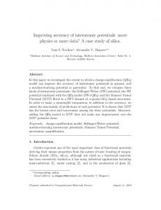
The first goal can be reached using suitable spatial access methods (see [SW 92] and [GB 90]). Such methods should efficiently support the selective spatial access to single objects as well as set-oriented access to large sets of objects caused by large data requests from secondary storage. In view of permanently increasing main memory sizes, the fast transfer of large, spatially adjacent object sets becomes more and more important. The second goal can be reached by using suitable objects representations in order to simplify the complex geometric algorithms. On the one hand, time consuming algorithms can be avoided by a geometric filter step based on object approximations [BKS 93a]. On the other hand, the processing of these algorithms can be simplified and speeded up by object decomposition techniques. Using object decompositions, geometric tests are applied only to components which are much more efficient than testing the whole object [Kri 91] and [KHS 91]. To decide which components are relevant for a particular test, a spatial access method has to organize the components of one object with respect to their location and shape [SK 91]. In this paper, we will present several research directions where a high potential can be found for substantial performance improvement of spatial query processing. We sketch the main concepts which in our point of view have to be integrated into spatial database systems in order to improve their query performance. The improvements are documented by experimental performance comparisons using real cartography data. The paper is organized as follows. First, we take a closer look at the execution of spatial queries and operations presenting the concept of multi-step query processing. In this section, we identify the main building blocks offering a high potential for speed up. In section 2, the first concept - geometric filtering - is discussed in detail. Afterwards, we describe the necessity of efficient transfer of the exact geometry from secondary storage to main memory and propose the concept of combining set I/O and spatial access methods. The exact geometry processing supported by decompositions is the topic of section 5. The rest of the paper contains a detailed discussion of spatial join processing. In particular, we investigate and evaluate spatial join processing supported by spatial access methods. The paper concludes with a brief statement of our findings and some suggestions for future work. 2 Multi-Step Spatial Query Processing Spatial database systems are used in very different application environments. Therefore, it is not possible to find a compact set of operations fulfilling all requirements of spatial applications. But as described in [BHKS 93], spatial selections are of great importance within the set of spatial queries and operations. They do not only represent an own query class, but also serve as a very important basis for the operations such as the nearest neighbor query and the spatial join. Therefore, an efficient implementation of spatial selections is an important requirement for good overall performance of the complete spatial database system. The two main representatives of spatial selections are the point and the region query (see figure 1): • Point Query Given a query point P and a set of objects M. The point query yields all the objects of M geometrically containing P (see figure 1(a)). • Region Query Given a polygonal query region R and a set of objects M, the region query yields all the objects of M sharing points with R. A special case of the region query is the window query. The query region of a window query is given by a rectilinear rectangle (see figure 1(b)). Both, the window query and the region query are often called range queries.
2
(b)
(a)
P
R
Fig. 1. Examples for a point and a window query For the efficient processing of spatial queries, we present a multi-step procedure (see figure 2). The main goal of our spatial query processor is to reduce expensive steps by preprocessing operations in the preceding steps which reduce the number of objects investigated in an expensive step. In figure 2, expensive steps are marked with a “$”-symbol. spatial query spatial query processor
spatial index
candidates geometric filter hits
false hits
candidates
I/O-transfer unit $ for exact geometry
exact geometry processor
$
false hits IDs of answers
geometry of answers
Fig. 2. Schematic diagram of multi-step spatial query processing A spatial selection is abstractly executed as a sequence of steps: First, we scale down the search space by spatial indexing. A spatial access method organizes pages containing sets of entries that consist of a geometric key, an object identifier (ID) and a reference to the exact object geometry. Due to the arbitrary complexity of real geographic objects, it is not advisable to build up an index using the complete geometric description of the objects as a key. Instead, approximations of the objects are used. Thus, the spatial access method is not able to yield the exact result of a query. However, because of the high selectivity of spatial queries a high number of objects is filtered out.
3
Pages containing results are transferred into main memory. If a page region fulfills the query condition (e.g. the whole page region is contained in the query window), all entries of the page correspond to correct answers of the query (hits). Otherwise, a page consists of entries which may fulfill the query. Therefore, we inspect these candidates using a geometric filter which tests the geometric key (or further approximations of the object geometry) against the query condition. As a result, we obtain three classes of objects: hits fulfilling the query, false hits not fulfilling the query and candidates possibly fulfilling the query. Geometric Filtering is cheap because it is performed on simple spatial objects and it saves query time because a lot of objects can be identified as false hits without transferring the exact geometry into main memory. Now, we have to distinguish two cases: In the first case, we are only interested in the object identifiers. Then, the hits are a subset of the set of answers (in figure 2 case 1 is indicated by a striped arrow). Only the candidates have to be transferred into main memory for further processing. In the other case, we require the complete object geometry as an answer to the query. Therefore, we need a transfer of the exact geometry of hits and candidates into main memory. The transfer of exact geometry may be very expensive because the exact representation of an object can be large (compare e.g. [BHKS 93]) and additionally for large window queries, large numbers of objects have to be transferred. In window queries the transferred objects are spatially adjacent. A physically contiguous storage of spatially adjacent objects is necessary to support a fast set-oriented access by the I/O-transfer unit. The other expensive step is processing the exact geometry of an object. After filtering, we have to investigate the remaining candidates. Using complex computational geometry algorithms, it is finally decided whether a candidate fulfills the query or not. Spatial access methods Considering spatial selections in more detail, it turns out that generally a small and locally restricted part of the complete search space has to be investigated. For an efficient scaling down of the search space, it is essential to use spatial access methods in the first step of our spatial query processor because high volumes of data have to be organized. Access methods as a part of the internal level of a database system are used to organize a dynamic set of objects on secondary storage. One-dimensional access methods like B-trees or linear hashing are not suitable for geographic database systems. For these systems, we have to provide data structures which organize the spatial objects with respect to their location and extension in the data space. Because of the arbitrary complexity of spatial objects, access methods for simpler two-dimensional objects like minimum bounding rectangles are widely discussed in the literature, e.g. the grid file, the quadtree, the buddy tree, the R-tree, and the R*-tree. Samet provides an excellent survey [Sam 90] of almost all of these methods. Simply stated, spatial access methods are based on point access methods using one of three techniques [SK 88]: Clipping partitions the data space into disjoint regions. The objects are associated with each of the regions they intersect and thus one object is stored in each of the corresponding blocks. In general, the technique of clipping may degrade query performance substantially since the number of objects (copies) to be stored increases which in turn increases the number of regions and thereby increasing the number of copies - a vicious circle. The transformation technique views an object as a point in some parameter space. Since transformations do not preserve the spatial neighborhood of objects in the original space, and since the distribution of parameter points is extremely skewed, the query efficiency tends to be quite low. The third technique is overlapping regions. In this technique each object is assigned to exactly one region. However, there may exist several regions potentially containing the searched object. Performance comparisons (e.g. [KSSS 89], [HS 92]) demonstrate that the well-known spatial access methods do not significantly differ in performance.We favour the R*-tree [BKSS 90], an improved variant of the well-known R-tree [Gut 84], because it is a simple, robust, and efficient spatial access method. This has been demonstrated in tests [BKSS 90] and in a comparison with
4
other access methods [HS 92]. The R*-tree uses the technique of overlapping regions and demonstrates that it is possible to organize spatial objects such that the overlap of the regions in the directory is extremely small. From our point of view, further research in spatial access methods will improve the overall-performance of query processing only marginally. In other words there is no potential for substantial performance improvements. Therefore, additional concepts have to be integrated into a spatial database system for improving its query performance. 3 Geometric Filtering As described above, spatial objects are organized and accessed by spatial access methods using geometric keys which maintain the most important features of the objects (position and extension). The smallest aligned rectangle enclosing an object, the minimum bounding rectangle (MBR), is the most popular geometric key. The MBR-approximation is unique and translational invariant but not rotational invariant. It can be computed with a simple linear algorithm which determines the minimum and maximum extension of the object in x- and y-direction. Using the MBR, the complexity of an object is reduced to four parameters. Inspecting the MBRs of the candidates against the spatial query condition, we obtain three classes of objects: hits fulfilling the query, false hits not fulfilling the query and remaining candidates possibly fulfilling the query (see figure 2). Using MBRs provides a fast but inaccurate filter for the response set. The larger the area of the MBR differs from the area of the original object, the more inaccurate is the geometric filtering, i.e. the candidate set includes a lot of false hits and the number of identified hits is very small. In order to get expressive and realistic results on the quality of the approximation when using MBRs, we investigated simple polygons with holes of various real maps. To be as general as possible, we used maps from different sources with different resolutions. The data files contain natural objects such as islands and lakes as well as administrative areas such as counties. Figure 3 depicts the analysed maps. Europe
BW
Lakes & Islands
Africa
Fig. 3. The analysed maps In the literature, several alternatives are proposed to measure the quality of approximations. In our application we are interested in measuring the accuracy of the geometric filter. The accuracy of the filter step is maximized by minimizing the deviation of the approximation from the original object. This deviation is measured by the false area of the approximation normalized to the area of the approximated object. Table 1 shows impressively that real cartography objects are only roughly approximated by MBRs. min
max
μ
σ/μ
Europe
0.25
21.14
0.93
0.21
BW
0.20
5.01
0.93
0.18
Lakes
0.21
22.11
0.97
0.32
Africa
0.34
5.64
0.89
0.23
• μ is the average of false area • σ/μ is the standard variation normalized to μ • min and max denotes the minimum and the maximum deviation of the area of the MBR from the area of the corresponding polygon occurring in the map, respectively.
Tab. 1. False area of the MBR-approximation normalized to the area of the object
5
This investigation was the starting point to look for other approximations which have a better approximation quality than the MBR. Approximations of objects which are used for geometric filtering should be simple to provide a fast filter (simplicity criterion) and they should have a high approximation quality (quality criterion) to reduce the number of false hits and to identify as many final answers as possible. In our point of view only convex approximations which can be represented by a small number of parameters are suitable candidates. Therefore, we tested the rotated minimum bounding rectangle (RMBR), the minimum bounding circle (MBC), the minimum bounding ellipse (MBE), the convex hull (CH), and the minimal enclosing convex n-corner (n-C). Rotated minimum bounding rectangle (RMBR) If we give up the restriction to align the MBR to the axes and allow rotations, the approximation quality of the MBR can be improved. Obviously, the resulting rotated MBR (RMBR for short) is additionally rotational invariant. It can be represented by the four parameters of the bounding rectangle and one more parameter that corresponds to the performed rotation. We use a simple algorithm with time complexity O(n2) to compute the RMBR. Minimum bounding circle (MBC) The circle needs three describing parameters (x-coordinate and y-coordinate of the center of the circle and the radius). The approximation with the minimum bounding circle is unique, translational invariant and rotational invariant. A deterministic linear algorithm was presented in [Meg 83] to determine the MBC. In our tests we used a randomized algorithm with an expected linear complexity [Wel 91] which is based on Seidel’s optimal linear algorithm [Sei 90]. A comparison of further methods can be found in [DF 91]. Minimum bounding ellipse (MBE) Any two-dimensional ellipse is determined by 5 parameters. Usually the ellipse is described by a symmetric matrix
A B B C
and the centre P = (p1, p2). The centre is the intersection of the semiaxis of
the ellipse and describes the position of the ellipse in the plane. The MBE-approximation is unique, translational and rotational invariant. A deterministic O(n2)-algorithm for computing the minimum bounding ellipse is presented in [Pos 84]. In our tests we used Welzl’s randomized algorithm [Wel 91] which has an expected linear complexity. Convex hull (CH) An obvious and popular approximation for simple polygons is the convex hull. The construction of the convex hull of a set of points is one of the best understood problems in computational geometry. We used Graham’s simple scan-algorithm [Gra 72] with time complexity O (n log n). The construction of the convex hull of a simple polygon is possible in O (n) time [Mel 87]. The required storage for the convex hull approximation is determined by the complexity of the object geometry and may vary from object to object. Minimum bounding n-corner (n-C) To obtain a predefined constant storage requirement, it is possible to compute the minimum bounding n-corner starting from the convex hull of the polygon. An algorithm to construct the n-C-approximation was proposed in [DB 83] for the first time. A detailed description and investigation of this algorithm is presented in [Sch 93]. Figure 4 visualizes the selected approximations using Great Britain as an example. These approximations differ especially in the approximation quality and storage requirement. The convex hull has the best approximation quality. The minimum bounding circle has the lowest storage requirement. First steps of an analytical and qualitative evaluation of approximations can be found in [Sch 92] and [Sch 93].
6
MBR
RMBR
MBC
MBE
CH Fig. 4. Different presented approximations
4-C
In [BKS 93a] we presented a detailed empirical investigation. The measured approximation qualities were almost independent of the various tested maps. Let us emphasize that this result is very interesting because we used maps from different sources with different resolutions (see figure 3). A clear order of rank turned out. Naturally, the convex hull has the best approximation quality (24 % false area), followed by the 5-corner (33 %), the 4-corner (44 %) and the rotated rectangle (62 %). Compared to the minimum bounding rectangle (93 %), clear gains of approximation quality were obtained. Obviously, the more parameters are used for the representation of an approximation, the better is the approximation quality. The results show that the approximation quality of the 5-corner is nearly the same as that of the convex hull. However, the storage requirement of convex hulls varies extremely and is on the average much higher than the storage requirement of the other approximations. The RMBR reduces the false area by 31 percentage points compared to the MBR, although only one additional parameter is used. The 5-corner needs 6 additional parameters compared to the MBR paying off in 60 percentage gain over the average false area of the MBR. Summarizing, we can state that the 5-corner yields the best trade-off between additional storage requirement and improvement of approximation quality. In order to integrate the 5-corner in geometric filtering of spatial query processing, two different ways can be followed. First, the common MBR remains the geometric key and the 5-corner is additionally stored in the data pages of the SAM. The advantage of this approach is obvious. The approximation quality is improved and all the known SAMs based on MBRs can be used. Second, we use the 5-corner as the geometric key and the MBR is not stored anymore. Doing this, we save storage, but SAMs using the transformation technique are not suitable. In [BKS 93a] we have shown that the 5-corner approximation can efficiently be organized in the R*-tree, a spatial access method originally designed for bounding rectangles. The simplicity and robustness of the spatial access method is preserved, because in the directory simple bounding
7
rectangles are organized and only in the data pages more complex approximations are stored. Obviously, in the filter step other approximations than the minimum bounding rectangle need more page accesses when traversing the SAM because of their higher storage requirement and their higher extension in x- and y-direction. However, the reduced number of false hits due to higher approximation quality results in a substantial gain in the geometry processor by avoiding time intensive computational geometry algorithms. This gain clearly exceeds the slightly higher access cost. 4 I/O-Transfer of Exact Geometry Most spatial access methods proposed up to now accommodate object approximations (e.g. minimum bounding rectangles) or a small number of spatial objects in their data pages. However, data pages storing spatially adjacent objects are distributed arbitrarily over the secondary storage. Typical range queries require the contents of many data pages to be retrieved from the database. This is much more expensive for arbitrarily distributed pages than for physically contiguous pages because the search time of a page on disk is much higher than the transfer time and because physically contiguous pages can be transferred by one set-oriented disk access into main memory (see [Wei 89]). In [HSW 88], Hutflesz et al. face the problem of global clustering of data pages using a multidimensional hashing scheme. The same concept is applied to minimum bounding rectangles in [HWZ 91]. However, the global clustering is preserved only for approximations of objects. Furthermore, this hash approach is not applicable to access methods with an arbitrary space partitioning scheme. In [BHKS 93], we demonstrated experimentally the necessity to integrate global clustering into query processing if large range queries occur. We compared three models for storing large sets of spatial objects: 1. Storing the exact object geometry outside of the spatial access method, e.g. in a sequential file. The main advantage of this scheme is the large number of approximations stored together in one data page. A fundamental drawback is the fact that the clustering just refers to the object approximations and not to the objects themselves. Consequently, when processing window queries, each access to an exact object geometry needs additional expensive search time. 2. Storing the exact object geometry inside the data pages of the spatial access method. Thus, spatial neighborhood is physically preserved at the level of exact object geometry. Objects within one data page are transferred into main memory just using one disk access. An essential drawback of this approach is the low number of objects fitting into one page. As a consequence, adjacent objects are often stored in different pages and clustering is restricted by the page size which is about 4 kbyte. 3. Our new approach, the scene organization, associates the geometry of spatially adjacent objects to sets of physically contiguous pages. These sets are derived from a slightly modified R*-tree and are called scenes. A scene is described by a minimum bounding rectangle. The geometric keys (and additional approximations) are organized in R*-trees as before. The scene organization allows dynamic changes of the database, supports large range queries as well as small queries, assures that a maximum scene size is not exceeded, and strives for a stable average scene size and a high storage utilization. A detailed algorithmic description of the scene organization is given in [BKS 93b]. A window query proceeds as follows: All scenes intersecting the query window are determined. If the degree of overlap between the scene and the query window is smaller than a heuristically determined query threshold, the window query is processed using the mechanism depicted in figure 2. Otherwise, the scene is completely transferred into main memory using the fast set-I/O [Wei 89]. Unfortunately, a scene may contain a number of false hits unnecessarily transferred into main memory. However, a relatively small number of false hits does not affect performance considerably, since the time needed for searching a page exceeds drastically the time for transferring a
8
page. After transferring the scene into main memory, the query works as usual without the transfer step after filtering. In figure 5, the three organization models are depicted.
SAM
SAM SAM
...
... data . . pages . ...
...
... ...
...
... data . . pages .
...
...
...
...
... ... data pages
...
...
scenes
external representation
model 1
model 2
model 3
Fig. 5. Organization models for storing spatial objects Realization of the scene organization Spatial access methods are very efficient for point queries and small range queries because they cluster objects in their data pages accordingly to their location in space. The idea of the scene organization is to cluster larger sets of spatial data on secondary storage in order to support large range queries. Therefore, we have to combine sets of pages by a strategy which is based on an efficient space partitioning scheme. Additionally, for large spatial units the design of a scene organization has to fulfill the following important requirements: • Due to the changes in the spatial database, a scene organization must be dynamic. • We want to support large range queries as well as small queries. Therefore, we need direct access to the scenes as well as a spatial index which supports an efficient spatial access to single objects in the database. • For the I/O-system it is easier to handle cluster units of equal size. Consequently, we assume that a maximum scene size exists. For achieving a predictable query behavior, we strive for a stable average scene size. Another important goal is a high storage utilization. Figure 6 depicts the schematic structure of our approach. We distinguish three parts: the scene descriptions are stored on the first level. A scene description consists of a geometric representation covering every spatial object of the corresponding scene. The scene description is supplemented by a pointer to a data structure organizing approximations and by the absolute address of the scene on secondary storage. The scene descriptions are organized in a data structure which is called scene tree. The spatial access methods handling the approximations of the spatial objects are called approximation trees. The relative address of the spatial object in the scene is assigned to every approximation. The scenes store the spatial objects for which internal clustering is maintained. Each scene is indexed by one approximation tree. The R*-tree [BKSS 90] is a spatial access method that clusters sets of spatial objects or their minimum bounding rectangles in its data pages. It uses a very efficient space partitioning scheme which neither clips nor transforms the spatial objects. Due to its good performance and its robustness, we take the R*-tree as a major component of our scene organization. We describe the scenes by their minimum bounding rectangles and organize them by a scene tree based on the R*-tree. We also use R*-trees as approximation trees. The approximation trees are necessary for two purposes: The first task is to organize the approximations in order to support an efficient access for spatial queries. Due to the efficient space partitioning scheme of the R*-tree, they are additionally used to determine new scenes as basic units for physical clustering.
9
scene tree Level of scene descriptions approximation trees Level of approximations ... physical clustering unit (scene)
Level of spatial objects
Fig. 6. Schematic structure of the scene organization (I) In order to demonstrate the high potential of performance gains for large range queries when applying the scene organization, we carried out a detailed empirical performance comparison of the three models using real test data. We used real test data from the US Bureau of the Census [Bur 89] containing county borders, highways, railway connections and rivers of four Californian counties. This database consists of 119,151 lines, each consisting of 2 to 349 points. Each co-ordinate is represented by a real number of 8 Bytes. Altogether the database has a size of 15.9 MByte. The lines were approximated by using minimal bounding rectangles. We investigated the performance improvement of the scene organization in comparison to the other two approaches. To compare the clustering of our scene organization with the other models, the access cost for point queries is a suitable measure. In the scene organization the cost of point queries is very close to the cost of the two other models. That means that the modifications of the R*-tree have almost no effect on its space partitioning. In table 2, a comparison of the access cost of the three models is presented by describing the speed up factor for query processing using model 2 and 3 in comparison to model 1. To investigate the performance of the models for large query regions, we carried out four test series with different sizes of the query regions. Each series consists of 464 quadratic window queries uniformly distributed over the data space covered by the objects. The area of the query regions varies between 0.25% and 16% of the data space. The cost for model 1 is standardized to “1”. For the other two models the numbers describe the speed up factor for query processing using these models. The average scene size for model 3 was 79,027 Bytes which was the scene size yielding the best results where we averaged over the four different sizes of the query windows. To evaluate the performance of the three models, we need a measure for the access cost. The time necessary for reading one page into main memory consists of the search time, i.e. the time needed for locating the page on secondary storage, and the transfer time, i.e. the time needed to transfer the data from secondary into main memory. If we normalize the cost for a transfer operation to 1, then in real magnetic disk drives the cost for a search operation is approximately 10 [PH 90]. Considering range queries, the access cost within the R*-tree is negligible in comparison to the access cost of the exact object representation. Thus, in the following, we take into account only the access cost for reading the exact object representation.
10
size of query windows (in% of data space)
0.25%
1: Geometry outside of the data pages
1%
4%
16%
1.0
1.0
1.0
1.0
2: Geometry inside the data pages
11.9
13.7
14.9
15.5
3: Scene organization
28.9
60.5
105.7
148.5
Tab. 2. Speed up factors for query processing using model 2 and 3 in comparison to model 1 Summarizing the results, we would like to point out the following statements: • Storing the exact object representation inside the data pages (model 2) speeds up query processing by a factor of 12 to 15 in comparison to model 1 (using separate pages). The size of the query regions has only a small influence on this factor. For the interpretation of the results, one remark is important: The objects used for the tests are relatively small in comparison to the size of the data pages. Using larger objects, i.e. objects larger than one data page, requires storing the exact representation outside of the data pages. As a consequence, query performance of model 2 comes closer to the performance of model 1. • The new scene organization is the clear winner of the performance comparison. Even the processing of small queries is performed considerably faster by this storage model. For small queries, we have a speed up factor of about 30 (in comparison to model 1) which is increasing to the impressive value of 148 for large queries. • Another important result is the fact that the optimal scene size is almost independent of the query sizes. Therefore, using the scene architecture with a fixed scene size is beneficial to queries of very different sizes. Furthermore, the flat form of the cost function guarantees a considerable speed up of the query processing, even if the average size of the scene is varying caused by insertions and deletions of objects. • Additionally, the scene organization efficiently supports small range queries. Even for point queries the performance of our new approach is not worse than the performance of conventional organization models. Global clustering has rarely been investigated in the area of spatial access methods although dramatic performance improvements can be achieved by using suitable techniques. In order to speed up set-oriented access to spatial objects for large range queries, we propose the scene organization, a new technique for global clustering in spatial database systems. Using this approach, large portions of the data are combined in scenes and spatially clustered on secondary storage. These scenes can be organized dynamically by using an R*-tree. Each scene is indexed by a separate R*-tree organizing the approximations of the spatial objects. Building up the scene organization, we maintain the clustering techniques of the R*-tree to a large extent in order to use the efficient space partitioning scheme of the R*-tree. For a fast transfer of scenes from secondary storage into main memory, the scene organization assumes that a set-oriented I/O-manager is available in the underlying system. In [BHKS 93], we presented the rough idea of the concept of a scene organization whereas in [BKS 93b] a detailed algorithmic realization of the scene organization is proposed. We performed the scene organization on top of the R*-tree. Based on an elaborated scene split, the scene organization is built up dynamically without global reorganization. The most important parameters for efficient processing of large range queries (scene size and query threshold) are determined experimentally. 5 Exact Geometry Processing Geometric filtering is based on object approximation and therefore determines a set of candidate objects that may fulfill the query condition. The geometry processor tests whether a candidate object actually fulfills the query condition or not. This step is very time consuming and dominates
11
spatial indexing and geometric filtering in many applications (see [BZ 91]). Algorithms from the area of computational geometry are proposed to overcome this time bottleneck. Different specialized data structures and techniques, such as plane sweep or divide-and-conquer, are used to design efficient algorithms for the different spatial queries and operations. Due to the complexity of the objects on the one hand and the selectivity of spatial queries on the other hand, it is useful to decompose the objects into simpler components because the decomposition substitutes complex computational geometry algorithms by multiple executions of simple and fast algorithms. The success of such processing depends on the ability to narrow down quickly the set of components that are affected by the spatial queries and operations. The performance comparisons in [KHS 91] demonstrate that decomposition techniques outperform the traditional undecomposed representation up to one order of magnitude for high selectivity queries. Consider a point-in-polygon test. For processing this test, an algorithm with linear runtime complexity is necessary [PS 88]. This examination of complex polygons i.e. polygons with thousands of vertices consumes a considerable amount of CPU time. On the other hand, only a small local part of the object is actually relevant for the decision whether an object contains a point or not. This leads to the idea of object decomposition. Applying this idea, the objects are divided into a number of simple and local components, e.g. triangles, trapezoids, convex polygons, etc. (see figure 7). During spatial query processing, only one or a small number of these components has to be checked. In [KHS 91] and [Kri 91] the decomposition approach for simple polygons with holes is presented and discussed in detail.
convex polygons
triangels
trapezoids
Fig. 7. Three decomposition techniques for simple polygons Using object decompositions, geometric tests are applied only to components, e.g. trapezoids, which is much more efficient than testing the whole polygon. To decide which components are relevant for a particular test, we use again an R*-tree to organize the components of one object with respect to their location and shape. In [SK 91] we proposed a new representation of a polygonal object called TR*-tree that efficiently supports various types of spatial queries and operations. The TR*-tree is a dynamic data structure that is persistently stored on secondary storage and is completely loaded to main memory for spatial query processing. In our approach using TR*-trees, we support efficiently the average case of various types of queries and operations in real applications where only one single representation of the objects is used. We decompose in a preprocessing step the polygonal objects into a minimum set of disjoint trapezoids using the plane-sweep algorithm proposed by Asano & Asano [AA 83]. However, we cannot define a complete spatial order on the set of trapezoids that are generated by this decomposition process. Thus, binary search on these trapezoids is not possible. Therefore, we propose to use the R*-tree for the spatial search. Due to its tree structure, the R*-tree permits logarithmic searching in the average case but due to the overlap within its directory, the search is not restricted to one path, and thus logarithmic search time cannot be guaranteed in the worst case. The R*-tree was designed as a spatial access method for secondary storage. In order to speed up the queries and operations mentioned above, we developed the TR*-tree, a variant of the R*-tree, designed to minimize the main memory operations and to store the trapezoids of the decomposed objects as complete objects without approximating them by minimum bounding rectangles. The performance of the TR*-tree cannot be proven analytically because the TR*-tree is a data structure that uses heuristic optimization strategies. Therefore, we are testing the performance of
12
the TR*-tree in an experimental analysis investigating real cartography data in a systematic framework. First results are reported in [SK 91]. For example, a point query on objects with 2,500 vertices is answered performing 20 point-in-MBR-tests and 3 point-in-trapezoid-tests. Compared to a linear point-in-polygon-test from the area of computational geometry, we have a speed up by a factor of 45. In [BKSS 93] we tested the TR*-tree approach to answer the spatial query whether two polygons are intersecting or not. The polygons had on the average about 1300 vertices. In comparison to a plane sweep algorithm, we measured performance improvements of a factor of 50. These results document impressingly that it is worth to integrate the approach of decomposition into spatial query processing. Further research on the trade-off between the complexity of the components and their number is reported in [SK 93]. 6 Spatial Join Processing In a database system, we can distinguish between two different types of queries. The one type of queries, called single-scan queries, requires at most one access to an object and therefore, the execution time is at most linear in the number of objects stored in the corresponding relation. Window queries are prime examples for single-scan queries in a spatial database system. In the previous sections, we discussed in detail the potential for improving query processing of single scan queries. The other type of queries are multiple-scan queries where objects have to be accessed several times and therefore, execution time is generally not linear but superlinear in the number of objects. For example, a join operation in a relational database system is a multiple-scan query. The most important multiple-scan query in a spatial DBS is the spatial join [Ore 86]. The spatial join can be used for implementing the map overlay in a GIS efficiently. The importance of the spatial join is comparable to the one of the natural join in a relational database system. The spatial join operation combines objects from two spatial relations according to their geometric attributes, i.e. their geometric attributes have to fulfill a spatial predicate. For example, consider the spatial relation Forests (Id, Name, FRegion) where the geometric attribute FRegion represents the borders of forests. The query “find all forests which are in a city” is an example of a spatial join on relations Forests and Cities. Here, the spatial predicate is whether a forest intersects a city. Definitions A relational θ-join of two relations A and B on columns i and j, denoted by A iθj B , combines those tuples where the i-th column of A and the j-th column of B fulfill the predicate θ. The most important join is the equijoin where θ is equality. A join A iθj B is called spatial join if the i-th column of A and the j-th column of B are sets of spatial objects and if θ is a spatial predicate [Gün 93]. The reader may think of the spatial objects as lines representing rivers, railway tracks and highways or as polygons representing a part of the surface of the earth. Spatial predicates may be intersection, containment or distance predicates. The most important spatial join is the intersection join where both columns are of a spatial type and θ is the intersection. In this section, we discuss only the intersection join. However, many of our results can be easily transferred to spatial joins using other spatial predicates. In an intersection the non-spatial attributes are not relevant for the join processing. Therefore, we omit non-spatial attributes and join two sets A = {a1,…,an} and B = {b1,…,bm} of spatial objects. In the following, we assume that the spatial access method maintains for each spatial object an entry which is (at least) a tuple (Id(a), Mbr(a), Ref(a)) where Id(a) is the unique identifier of the spatial object a in the database, Mbr(a) is the minimum bounding rectangle of a used in the SAM as geometric key, and Ref(a) refers to the exact geometry of the object a. Now, we can distinguish the following variants of the intersection join: • MBR-join: Compute all pairs (Id(ai), Id(bj)) with Mbr(ai) ∩ Mbr(bj) ≠ ∅ • object-join: Compute all pairs (Id(ai), Id(bj)) with ai ∩ bj ≠ ∅
13
Contrary to relational joins, these two variants compute only the identifiers of the objects. The reason is the complexity of a spatial object: only when the user or the application really needs the geometry of an object, it should be transferred into main memory. Note that the MBR-join can be used for implementing the filter step of the object-join. This explains the importance of the MBRjoin. The object-join itself is the base for computing the intersection overlay of the spatial objects: • intersection overlay: Compute ai ∩ bj with ai ∩ bj ≠ ∅ The intersection overlay does not only compute the identifiers of the objects in the response set but also the resulting objects. In this section, we restrict our considerations to the MBR-join. Although the MBR-join is less complex than other types of spatial joins, almost all methods designed for an efficient join processing of non-spatial relations, see [ME 92] for a survey, cannot be efficiently used for MBR-joins. Using the simple nested loop approach, the MBR of all spatial objects of the one relation has to be checked against the MBRs of all objects of the other relation. Since we consider very large relations of spatial objects, the performance of the nested loop algorithm is not acceptable. Hashed-based join algorithms are suitable only for natural and equijoins but not for any type of spatial join. Another approach is similar to a sort-merge join. Here, the MBRs of spatial objects are sorted according to their spatial proximity. This approach for processing an MBR-join may be considered if there is not already a spatial index on the spatial relations. However, our basic assumption is that a spatial access method efficiently supports queries on the set of MBRs (and therefore, indirectly on the spatial relations). Thus, we are interested in exploiting spatial access methods for an efficient processing of MBR-joins. There are several other approaches for performing natural joins using multidimensional point access methods, e.g. grid files [Bec 92] and kd-trees [HNKT 90]. These methods can be used for MBR-joins, if rectangles are transformed to higher dimensional points. However, the most serious disadvantage is that the use of transformation does not preserve proximity. In the following, we restrict our considerations to R-trees [Gut 84], particularly R*-trees [BKSS 90], used as the underlying spatial access method for processing MBR-joins. It has been shown in [BKSS 90] that the R*-tree is one of the most efficient members of the R-tree family with respect to several single-scan queries. Since several geographic information systems, e.g. Intergraph’s GIS, and DBSs, e.g. Postgres [SRH 90], use R-trees as their basic spatial access method, there is also considerable interest in efficient join algorithms using R-trees. An R-tree is a B+-tree like access method that stores multidimensional rectangles as complete objects without clipping them or transforming them to higher dimensional points. A non-leaf node contains entries of the form (ref, rect) where ref is the address of a child node and rect is the minimum bounding rectangle of all rectangles which are entries in that child node. A leaf node contains entries of the same form where ref refers to a spatial object in the database and rect is the minimum bounding rectangle of that spatial object. Let us mention, that storing spatial objects instead of references in leaf nodes do not affect the basic algorithms of the R-tree. Given an entry E of a node, E.rect and E.ref denote the corresponding rectangle and reference, respectively. Let M be the number of entries that fit in a node and let m be a parameter specifying the minimum number of entries in a node, 2 ≤ m ≤ ⎡M/2⎤. An R-tree satisfies the following properties: • The root has at least two children unless it is a leaf. • Every node contains between m and M entries unless it is the root. • The tree is balanced, i.e. every leaf node has the same distance from the root. • Every rectangle of a non-leaf node covers all rectangles in its corresponding child node. In general, the rectangle is even the minimum bounding rectangle. Since one node of the data structure corresponds exactly to one page on secondary storage, we will use both terms synonymously in the following. An R-tree is completely dynamic; insertions and deletions can be intermixed with queries without any global reorganization. Although data entries are grouped together according to the location
14
of their rectangles in space, R-trees have to allow overlap in directory nodes, i.e. rectangles of different entries may have a common intersection. Since a high overlap results in poor query performance, one of the most important design goals of the R*-tree was the reduction of overlap. Similar to B-trees, R-trees guarantee that storage utilization is at least m/M and that the height grows logarithmically in the number of data records. The reader is referred to the original papers [Gut 84] and [BKSS 90] for a more detailed discussion. Cost and Performance Measures For an R*-tree R we use the following notations: |R|dir (|R|dat) = number of directory (data) pages ||R||dir (||R||dat) = number of directory (data) entries Obviously, the total number |R| of pages is given by |R|dat + |R|dir. Analogously, the total number ||R|| of entries is given by ||R||dat + ||R||dir. Now, let us consider two sets of rectangles each of them being organized by an R*-tree. In the following, we call the R*-trees R and S. As a performance measure for the execution time of a MBR-join between R and S, we use CPU-time as well as I/O-time. Only the number of disk accesses is not sufficient to measure execution time of joins, particularly of spatial joins, appropriately. Already in case of natural joins, the number of tests for the join condition has essential influence on the execution time. To check the join condition in case of spatial joins is far more expensive than in case of natural-joins. Therefore, a good measure for performance consists of both, the number of disk accesses and the number of comparisons. The I/O-time is usually measured in the number of disk accesses required for performing the join. A similar performance measure is used in the following. Since the I/O-time for reading and writing a page slightly depends on the size of the page, we differentiate between the positioning cost (including seek cost and rotational latency) and transfer cost. In order to reduce I/O-operations, a buffer can be used. Independent of the size of a buffer, any processing of an MBR-join will read each required page at least once into main memory. If all pages are required for a join, a lower bound for the I/O-cost is |R|dat + |S|dat. This result is wellknown as the minimum cost for a natural-join using two B-trees. In case of R*-trees, however, it might be possible that a MBR-join requires less than |R|dat + |S|dat pages. The reason is that the union of all directory rectangles with the same distance from the root of the R*-tree does not completely cover the underlying data space. The CPU-time of an MBR-join is measured in the number of floating point comparisons. Comparisons are required for checking the join condition, i.e. whether two rectilinear rectangles intersect. Note, that for a pair of rectilinear rectangles four comparisons are exactly required to determine that the join condition is fulfilled. If the rectangles do not fulfill the join condition, less than four comparisons might be required. There are many other operations affecting CPU-time, but in general they do not asymptotically influence CPU-time. An analytical investigation of the execution time of an MBR-join performed with R*-trees seems to be almost impossible. Not surprisingly, there are only a few analytical results known for spatial access methods. Most of these analytical results are restricted to multidimensional points, to single-scan queries, and to uniformly distributed data set very rarely occurring in real applications. Therefore, in [BKS 93c] we investigate MBR-joins in an empirical comparison using cartographic maps from real applications. We consider two files with 131,461 and 128,971 line objects in an area of California. The data is drawn from the TIGER/Line files used by the US Bureau of the Census (1989). The first map represents streets, whereas the second map represents rivers and railway tracks. For each of the maps, the minimum bounding rectangles of the polygonal objects are stored in an R*-tree. The join of R and S results in a response set of 86,094 pairs of intersecting rectangles. For various page sizes, the most important properties of R*-trees R and S are reported in table 3.
15
page size
M
1 KByte 2 KByte 4 KByte 8 KByte
51 102 204 409
R*-tree R R*-tree S height |R|dir |R|data height |S|dir 4 127 4,202 4 117 3 33 2,143 3 30 3 9 1,069 3 8 3 3 541 3 3
|S|data 3,996 1,991 1,005 495
|R|+|S| 8,442 4,197 2,091 1,042
Tab. 3. Properties of R*-trees R and S The conventional approach of an MBR-join for R*-trees The basic idea of performing a MBR-join with R*-trees is to use the property that directory rectangles form the minimum bounding rectangle of the data rectangles in the corresponding subtrees. Thus, if the rectangles of two directory entries ER and ES do not have a common intersection, there will be no pair (rectR, rectS) of intersecting data rectangles where rectR is in the subtree of ER and rectS is in the subtree of ES. Otherwise, there might be a pair of intersecting data rectangles in the corresponding subtrees. In the following, we assume that both trees are of the same height. The case of joining R*-trees of different height is discussed in [BKSS 93]. The following algorithm presents the conventional approach: MBR_J1 (R,S: R_Node); (* height of R is equal height of S *) FOR (all ES ∈S) DO FOR (all ER ∈R with ER.rect ∩ ES.rect ≠ ∅) DO IF (R is a leaf page) THEN (* (S is also a leaf page) *) output (ER,ES) ELSE ReadPage(ER.ref); ReadPage(ES.ref); MBR_J1(ER.ref,ES.ref) END END END END MBR_J1;
Here, it is assumed that R_Node is the type of a node in an R*-tree and that each node accommodates a collection of entries. As previously introduced, an entry E consists of a pointer ref and a rectangle rect. A procedure ReadPage is assumed to read the required page from the buffer or, if the page is not in the buffer, from secondary storage. The algorithm recursively traverses both of the trees in top-down fashion. The R*-tree makes use of a so-called path buffer accommodating all nodes of the path which was accessed last. In order to be more efficient with respect to I/O, an additional buffer is used for single pages, not complete paths, independently of the path buffer. The buffer, called LRU-buffer, follows the last recently used policy. The reason for two different buffers is that the path buffer exclusively belongs to the data structure (i.e. R*-tree), whereas the LRU-buffer is considered as a buffer of the underlying system. Note, that in a multiuser environment, a spatial join operation can only occupy a “small” fraction of the LRU-buffer. To which extend the LRU-buffer is used in a spatial join, depends on the system load. In our experiments, we assume that the R*-trees involved in the MBR-join exclusively use all pages of the LRU-buffer. In table 4, we report the results of the algorithm MBR_J1 using R*-trees R and S as input. The MBR-join is performed with various page sizes and various buffer sizes. The largest considered buffer size corresponds to keeping about 6% of both R*-trees in main memory. For todays computer system, this seems to be a realistic assumption. For each setting, we report the number of disk accesses required to compute the join. Additionally, we keep track of the number of comparisons
16
required for checking the join condition. This number is reported in the last row of table 4. Note, that this number is independent of the size of the LRU-buffer. Size of pages 2 KByte 4 KByte 8 KByte 12,479 5,720 2,837 12,010 5,720 2,837 9,589 5,454 2,822 6,299 4,474 2,676 4,964 2,768 2,181 4,197 2,091 1,042 65,807,555 118,864,748 242,728,164
1 KByte 24,727 20,318 13,803 11,359 10,372 8,442 33,566,961
0 8 Size of LRU-buffer 32 (KByte) 128 512 opt. buffer size # comparisons
Tab. 4. Number of disk accesses and comparisons required for MBR_J1 Let us first discuss the results without using an LRU-buffer, i.e. buffer size = 0. For all sizes of pages, a page of the R*-tree is read into main memory on the average only about three times. For these specific files, the overlap of the R*-tree seems to have not much influence on the performance of the join. Now let us consider the cases of using small LRU-buffers. For a small page, the LRU-buffer pays off even if it is very small. For a 32 KByte LRU-buffer, the number of disk accesses is only 55% of the number required by the join without any LRU-buffer. For larger page sizes, the same effect can only be observed in case of also using a large buffer. In order to determine whether the MBR-join is CPU-bound or I/O-bound, we have estimated the execution time of the MBR-join charging 1.5*10-2 seconds for positioning the disk arm, 0.5*10-3 seconds for transferring 1 KByte of data from disk and, 3.9*10-6 seconds for a floating point comparison (including necessary overhead). The last number is determined experimentally and depends obviously on the underlying hardware. For performing the experiments, we used HP720 workstations which deliver on 57 MIPs and 17.9 MFlops. Moreover, the positioning cost for moving the disk arm to the position of the desired page depends on the specific disk, how well the spatial relations are clustered on disk and on the load of the disk during performing the join. Using the results of table 4, we have computed the time estimates presented in figure 8. time (sec) 1000 800 600 400
page size:
1 KByte
2 KByte
4 KByte
512
128
8
32
0
512
128
8
32
0
512
128
8
32
0
512
128
8
32
0 buffer size (KByte)
0
200
8 KByte
I/Otime
1000
time (sec) buffer size = 128 KByte 500
CPUtime
0
page size 1 KB
2 KB
4 KB
8 KB
Fig. 8. Estimation of the execution time of MBR_J1 As demonstrated in the upper diagram of figure 8, best overall performance is achieved for page sizes of 1 and 2 KByte. The lower diagram shows that the MBR-join is slightly I/O-bound for a page size of 1 KByte. However, with increasing page size, the MBR-join is becoming more and
17
more CPU-bound. This observation is true for small and large LRU-buffers. Hence, we can state that cost optimization of a MBR-join has to take into account both, CPU- and I/O-time. There are at least two parts in the algorithm MBR_J1 which are worth to be improved. First, CPU-time consumption is rather high since each entry of the one node is checked against all entries of the other node. Second, pages are selected for the next call of MBR_J1 without taking into account the I/O-cost for reading these pages. A better approach would be to compute the “best” sequence of pairs of pages required for computing the join on the next level of the R*-tree. In [BKS 93c] a new spatial join algorithm is proposed which improves CPU-time dramatically using the techniques of spatial sorting and restricting the search space. Moreover, I/O-performance has been improved by determining how the required pages are read into the buffer. Our suggested policies are based on spatial locality, such that the pages required for computing an answer to the spatial join are already in the buffer with high probability. In an experimental performance comparison using large relations of real data, we showed that our suggested techniques improve the execution time of the conventional approach by factors. In order to investigate whether our test results depend on the particular data, we have performed several MBR-joins with various spatial relations obtained from real geographic applications. In table 5, we report the most import characteristics of our tests (A) to (E). For test (D), we have performed an MBR-join with two identical R*-trees. Nevertheless, our algorithms treated the R*-trees as if they would be different. For test (E), region data instead of line data was used for performing MBR-joins [Sta 90].
(A) (B) (C) (D) (E)
R*-tree R ||R||dat 131,461 131,461 598,677 128,971 67,527
R*-tree S ||S||dat 128,971 131,192 128,971 128,971 33,696
subject of map streets streets streets rivers & railways region data
subject of map rivers & railways streets rivers & railways rivers & railways region data
intersections 86,094 154,262 395,189 505,583 543,069
Tab. 5. Characteristics of R*-trees in tests A - E In figure 9, we depict the improvement factor how many times the new algorithm performs better than MBR_J1 for different page sizes. We have assumed a buffer size of 128 KByte. The results confirm that the factors of performance improvement are not dependent on the test data. 15.00
A
buffer size = 128 KByte B
10.00
C 5.00 D 0.00 1 KByte
2 KByte
4 KByte
8 KByte
E
Fig. 9. Improvement factors for different real test data In our future work, we are particularly interested in a more detailed study of spatial joins. In this section, we put our emphasis on the MBR-join which computes the spatial join of the minimum bounding rectangles of the spatial objects. We are in the process of investigating more complex types of spatial joins which actually operate on the real spatial objects. For example, in [BKSS 93] we present a multi-step spatial join processor for the object join in which sophisticated geometric
18
filtering and exact geometry processing is integrated. In our point of view spatial join processing is the area with the highest potential for performance improvements. Performance gains up to three orders of magnitude are realistic for complex polygons with more than 1000 vertices (see [BKSS 93]). 7 Conclusions In this paper, we pointed out that for improving query performance in spatial database systems two properties are an absolute necessity: (i) a fast spatial access to the objects and (ii) a fast processing of geometric operations. Starting point of our considerations was the well-established fact that a fast spatial access can only be achieved by integrating spatial access methods (SAMs) into spatial database systems. Performance comparisons ([KSSS 89], [HS 92]) demonstrate that the well-known SAMs do not significantly differ in performance. From our point of view, further research in designing new SAMs will improve the overall-performance of query processing only marginally. We hopefully convinced the reader that it is more fruitful to optimize existing SAMs - e.g. the R*-tree - with respect to complex spatial queries than to suggest completely new SAMs. The most popular approach for handling complex spatial objects is to use their minimum bounding rectangles as a geometric key in a spatial access method. Obviously, this rough approximation provides a fast but inaccurate filter for the set of answers to a query. The better the quality of the approximation is, the faster query processing can be performed. We investigated six different types of approximations with respect to their query performance. As a result of our empirical comparison it turns out that, depending on the complexity of the objects and the type of queries, the approximation 5-corner clearly outperforms the popular minimum bounding rectangle. In a set-oriented access to large sets of objects, e.g. large window queries, high volumes of spatially adjacent objects have to be transferred into main memory. Therefore, a physically contiguous storage of spatially adjacent objects - global clustering - is necessary to support a fast set-oriented access to large sets of results. This aspect of spatial query processing has rarely been investigated although this I/O-intensive transfer offers a high potential for performance improvement. We described the scene organization - a technique for supporting efficient set-oriented access to spatial data. Empirical comparisons showed that the scene organization improves query performance dramatically with respect to the conventional approach. For a fast transfer of scenes from secondary storage into main memory, the scene organization assumes that a set-oriented I/O-manager is available in the underlying system. Due to the complexity of the objects on the one hand and the selectivity of spatial queries on the other hand, it is useful to decompose the objects into simpler components because the decomposition substitutes complex computational geometry algorithms by multiple executions of simple and fast algorithms. The usage of TR*-trees - a data structure organizing decomposition components facilitates a fast search on the set of components that are affected by the spatial queries and operations. Performance comparisons with real cartography data indicate that decomposition techniques outperform the traditional undecomposed representation up to one or two orders of magnitude depending of the complexity of the spatial objects. Finally, we showed how the R*-tree can be exploited adequately for improving the expensive spatial join. We described a new MBR-join algorithm and showed that our suggested techniques improve the execution time of the standard approach by factors of up to 15. In our point of view, the spatial join is such an important operation in spatial database systems that the fine tuning of spatial join processing is an absolute necessity. In future research work, not only the MBR-join has to be improved but also the more time intensive object-join and overlay-join.
19
References [AA 83]
Asano Ta., Asano Te.: ‘Minimum Partition of Polygonal Regions into Trapezoids’, Proc. 24th IEEE Annual Symp. on Foundations of Computer Science, 1983, pp. 233-241. [Bec 92] Becker, L. A.: ‘A New Algorithm and a Cost Model for Join Processing with Grid Files’, PhD-thesis, University of Siegen, 1992. [BHKS 93] Brinkhoff T., Horn H., Kriegel H.-P., Schneider R.: ‘A Storage and Access Architecture for Efficient Query Processing in Spatial Database Systems’, Proc. 3rd Int. Symp. on Large Spatial Databases, Singapore, 1993. [BKS 93a] Brinkhoff T., Kriegel H.-P., Schneider R.: ‘Comparison of Approximations of Complex Objects used for Approximation-based Query Processing in Spatial Database Systems’, Proc. 9th Int. Conf. on Data Engineering, Vienna, Austria, 1993. [BKS 93b] Brinkhoff T., Kriegel H.-P., Schneider R.: ‘Scene Organization: A Technique for Global Clustering in Spatial Database Systems’, 1993, submitted for publication. [BKS 93c] Brinkhoff T., Kriegel H.-P., Seeger B.: ‘Efficient Processing of Spatial Joins Using R-trees’, Proc. ACM/SIGMOD Int. Conf. on Management of Data, Washington D.C., 1993. [BKSS 90] Beckmann N., Kriegel H.-P., Schneider R., Seeger B.: ‘The R*-tree: An Efficient and Robust Access Method for Points and Rectangles’, Proc. ACM SIGMOD Int. Conf. on Management of Data, Atlantic City, NJ., 1990, pp. 322-331. [BKSS 93] Brinkhoff T., Kriegel H.-P., Schneider R., Seeger B.: ‘Multi-Step Spatial Join Processing’, 1993, submitted for publication. [Bur 89] Bureau of the Census: ‘TIGER/Line Percensus Files, 1990 Technical Documentation’, Washington, D.C., 1989. [BZ 91] Benson D., Zick G.: ‘Symbolic and Spatial Database for Structural Biology’, Proc. OOPSLA, 1991, pp. 329-339. [CDRS 86] Carey M. J., DeWitt D. J., Richardson J. E., Shekita E. J.: ‘Object and File Management in the EXODUS Extensible Database System’, Proc. 12th Int. Conf. on Very Large Data Bases, Kyoto, Japan, 1986, pp. 91-100. [DB 83] Dori D., Ben-Bassat M.: ‘Circumscribing a Convex Polygon by a Polygon of Fewer Sides with Minimal Area Addition’, Computer Vision, Graphics, and Image Processing, Vol. 24, 1983, pp. 131-159. [DF 91] Dörflinger J., Forst W.: ‘Approximation durch Kreise: Verfahren zur Berechnung der Hüllkugel’, Manuscript, 1991. [GB 90] Günther O., Buchmann A.: ‘Research Issues in Spatial Databases’, Proc. IEEE CS Bulletin on Data Engineering, Vol. 13, No. 4, 1990, pp. 35-42. [Gra 72] Graham R. L.: ‘An Efficient Algorithm for Determining the Convex Hull of a Finite Planar Set’, Info. Proc. Letters, Vol. 1, 1972, pp. 132-133. [Gün 93] Günther, O.: ‘Efficient Computations of Spatial Joins’, Proc. 9th Int. Conf. on Data Engineering, Vienna, Austria, 1993. [Gut 84] Guttman A.: ‘R-trees: A Dynamic Index Structure for Spatial Searching’, Proc. ACM SIGMOD Int. Conf. on Management of Data, Boston, MA., 1984, pp. 47-57. [Güt 89] Güting R. H.: ‘Gral: An Extensible Relational Database System for Geografic Applications’, Proc. 15th Int. Conf. on Very Large Data Bases, Amsterdam, Netherland, 1989, pp. 33-44. [HNKT 90] Harada L., Nakano M., Kitsuregawa M., Takagi M.: ‘Query Processing Methods for Multi-Attribute Clustered Relations’, Proc. 16th Int. Conf. on Very Large Data Bases, Brisbane, 1990, pp. 59-70. [HS 92] Hoel E.G., Samet H.: ‘A Qualitative Comparison Study of Data Structures for Large Line Segment Databases’, Proc. SIGMOD Conf., San Diego, CA., 1992, pp 205-214. [HSW 88] Hutflesz A., Six H.-W., Widmayer P.: ‘Globally Order Preserving Multidimensional Linear Hashing’, Proc. 4th Int. Conf. on Data Engineering, Los Angeles, CA., 1988, pp. 572-579. [HWZ 91] Hutflesz A., Widmayer P., Zimmermann C.: ‘Global Order Makes Spatial Access Faster’, Int. Workshop on Database Management Systems for Geographical Applications, Capri, Italy, 1991, in: Geographic Database Management Systems, Springer, 1992, pp. 161-176. [KHS 91] Kriegel H.-P., Horn H., Schiwietz M.: ‘The Performance of Object Decomposition Techniques for Spatial Query Processing’, Proc. 2nd Symp. on the Design of Large Spatial Databases, Zürich, Switzerland, 1991, in: Lecture Notes in Computer Science, Vol. 525, Springer, 1991, pp. 257-276.
20
[KSSS 89]
[Kri 91]
[ME 92] [Meg 83] [Mel 87] [Ore 86] [Pau 87]
[PH 90] [Pos 84] [PS 88] [Sam 90] [Sch 92]
[Sch 93] [Sei 90] [SK 88] [SK 91]
[SK 93] [SR 86] [SRH 90] [Sta 90] [SW 92] [Wei 89] [Wel 91] [Wid 91]
Kriegel H.-P., Schiwietz M., Schneider R., Seeger B.: ‘Performance Comparison of Point and Spatial Access Methods’, Proc. 1st Symp. on the Design and Implementation of Large Spatial Databases, Santa Barbara, CA., 1989, in: Lecture Notes in Computer Science, Vol. 409, Springer, 1990, pp. 89-114. Kriegel H.-P., Heep P., Heep S., Schiwietz M., Schneider R.: ‘An Access Method Based Query Processor for Spatial Database Systems’, Int. Workshop on Database Management Systems for Geographical Applications, Capri, Italy, 1991, in: Geographic Database Management Systems, Springer, 1992, pp. 273-292. Mishra P., Eich M.H.: ‘Join Processing in Relational Databases’, ACM Computing Surveys, Vol. 24, No. 1, 1992, pp. 63-113. Megiddo N.: ‘Linear-time Algorithms for Linear Programming in R3 and Relates Problems’, SIAM Journal Comput., Vol. 12, 1983, pp. 759-776. Melkman A.A.: ‘On-line Construction of the Convex Hull of a Simple Polyline’, Information Processing Letters, Vol. 25, No. 1, 1987, pp. 11-12. Orenstein J. A.: ‘Spatial Query Processing in an Object-Oriented Database System’, Proc. ACM SIGMOD Int. Conf. on Management of Data, Washington D.C., 1986, pp. 326-333. Paul H.-B., Schek H.-J., Scholl M.S., Weikum G., Deppisch U.: ‘Architecture and Implementation of the Darmstadt Database Kernel System’, Proc. ACM SIGMOD Int. Conf. on Management of Data, San Francisco, CA., 1987, pp. 196-207. Paterson D., Hennessy J.: ‘Computer Architecture: A Quantitative Approach’, Morgan Kaufman, 1990. Post M.J.: ‘Minimum Spanning Ellipsoids’, Proc. 16th Annual Symp. on Theory of Computing, 1984, pp. 108-116. Preparata F. P., Shamos M. I.: ‘Computational Geometry’, Springer, 1988. Samet H.: ‘The Design and Analysis of Spatial Data Structures’, Addison Wesley, 1990. Schneider R.: ‘A Storage and Access Structure for Spatial Database Systems’, Ph.D.-thesis (in German), Institute for Computer Science, University of Munich, 1992; will be published by BI Wissenschaftsverlag. Schiwietz M.: ‘Storage and Query Processing of Complex Spatial Objects’, Ph.D.-thesis (in German), Institute for Computer Science, University of Munich, 1993. Seidel R.: ‘Linear Programming and Convex Hulls made Easy’, Proc. 6th Annual ACM Symp. on Computational Geometry, Berkeley, CA., 1990, pp. 211-215. Seeger B., Kriegel H.-P.: ‘Techniques for Design and Implementation of Efficient Spatial Access Methods’, Proc. 14th Int. Conf. on Very Large Databases, Los Angeles, CA., 1988, pp. 360-371.. Schneider R., Kriegel H.-P.: ‘The TR*-tree: A New Representation of Polygonal Objects Supporting Spatial Queries and Operations’, Proc. 7th Workshop on Computational Geometry, Bern, Switzerland, 1991, in: Lecture Notes in Computer Science, Vol. 553, Springer, 1991, pp. 249-264. Schiwietz M., Kriegel H.-P..: ‘Query Processing of Spatial Objects: Complexity versus Redundancy’, Proc. 3rd Int. Symp. on Large Spatial Databases, Singapore, 1993. Stonebraker M., Rowe L.: ‘The Design of POSTGRES’, Proc. ACM SIGMOD Conf. on Management of Data, Washington D.C., 1986, pp. 340-355. Stonebraker M., Rowe L., Hirohama M.: ‘The Implementation of POSTGRES’, IEEE Trans. on Knowledge and Data Engineering, Vol. 2, No. 1, 1990, pp. 125-142. Statistical Office of the European Communities: ‘Regions’, 1990. Six H.-W., Widmayer P.: ‘Spatial Access Structures for Geometric Databases’, Data Structures and Efficient Algorithms, Lecture Notes in Computer Science, Vol. 594, 1992, pp. 214-232. Weikum G.: ‘Set-Oriented Disk Access to Large Complex Objects’, Proc. 5th Int. Conf. on Data Engineering, Los Angeles, CA., 1989, pp. 426-433. Welzl E.: ‘Smallest Enclosing Disks (Balls and Ellipsods), Paper B91-09, Free University of Berlin, 1991. Widmayer P.: ‘Data Structures for Spatial Databases’ (in German), in: Vossen G., Witt K.-U. (eds.): ‘Entwicklungstendenzen bei Datenbank-Systemen’ (Future Trends in Database Systems), Oldenbourg, 1991, pp. 317-361.
21