(specifically, of connectivity games on bounded layer graphs), there does exist a polynomial algorithm to ... We call pi the payoff of agent ai, and denote the ...
Power in Threshold Network Flow Games Yoram Bachrach, Jeffrey S. Rosenschein School of Engineering and Computer Science Hebrew University, Jerusalem, Israel {yori, jeff}@cs.huji.ac.il
Abstract Preference aggregation is used in a variety of multiagent applications, and as a result, voting theory has become an important topic in multiagent system research. However, power indices (which reflect how much “real power” a voter has in a weighted voting system) have received relatively little attention, although they have long been studied in political science and economics. We consider a particular multiagent domain, a threshold network flow game. Agents control the edges of a graph; a coalition wins if it can send a flow that exceeds a given threshold from a source vertex to a target vertex. The relative power of each edge/agent reflects its significance in enabling such a flow, and in real-world networks could be used, for example, to allocate resources for maintaining parts of the network. We examine the computational complexity of calculating two prominent power indices, the Banzhaf index and the Shapley-Shubik index, in this network flow domain. We also consider the complexity of calculating the core in this domain. The core can be used to allocate, in a stable manner, the gains of the coalition that is established. We show that calculating the Shapley-Shubik index in this network flow domain is NP-hard, and that calculating the Banzhaf index is #P-complete. Despite these negative results, we show that for some restricted network flow domains there exists a polynomial algorithm for calculating agents’ Banzhaf power indices. We also show that computing the core in this game can be performed in polynomial time.
1
Introduction
Social choice theory can serve as an appropriate foundation upon which to build multiagent applications. There is a rich literature on the subject of
1
voting1 from political science, mathematics, and economics, with important theoretical results. Builders of automated agents can benefit from this work as they engineer systems that reach group consensus. Interest in the theory of economics and social choice has in fact become widespread in computer science, because it is recognized as having direct implications on the building of systems comprised of multiple automated agents [30, 9, 37, 31, 26, 15, 28]. What distinguishes computer science work in these areas is its concern for computational issues: how are results arrived at (e.g., equilibrium points)? What is the complexity of the process? Can complexity be used to guard against unwanted phenomena? Does complexity of computation prevent realistic implementation of a technique? The practical applications of voting among automated agents are already widespread. Ghosh et al. [12] built a movie recommendation system; a user’s preferences were represented as agents, and movies to be suggested were selected through agent voting. Candidates in virtual elections have also been beliefs, joint plans [10], and schedules [14]. In this paper, we consider a topic that has been less studied in the context of automated agent voting, namely power indices, which attempt to measure the control a voter has over decisions of a larger group. Two popular power indices are the Shapley-Shubik power index and the Banzhaf power index. While such indices have mostly been used for measuring power in weighted voting systems, they are well-defined for any simple coalitional game, and can thus be easily adapted for other domains as well. We look at some computational aspects of the Banzhaf and ShapleyShubik power indices in a specific environment, namely a threshold network flow game—TNFG. In this game, a coalition of agents wins if it can send a flow of size at least k from a source vertex s to a target vertex t, with the relative power of each edge reflecting its significance in allowing such a flow. This is a threshold variant of the cardinal network flow game—CNFG, where the utility of a coalition is the maximal flow it can send between the source and the target. We first show that although TNFG and CNFG appear to be very similar, the computational difficulty of certain problems can be different for these two domains. First, we show that while it is easy to test whether a certain agent is a dummy in CNFG, it is coNP-complete to do so in TNFGs. We then use this result to show that calculating the Shapley-Shubik power index is NPhard in TNFGs. We provide a stronger result for the Banzhaf power index 1 We use the term in its intuitive sense here, but in the social choice literature, “preference aggregation” and “voting” are basically synonymous.
2
in TNFGs, and show that it is #P-complete to compute it. Despite these negative results, we show that for some restricted network flow domains (specifically, of connectivity games on bounded layer graphs), there does exist a polynomial algorithm to calculate the Banzhaf power index of an agent. These game theoretic solution concepts have applications in real-world networks. For example, the power index might be used to allocate maintenance resources (a more “powerful” edge being more critical), in order to maintain a given flow of data between two points. Thus, analyzing the complexity of calculating power indices and providing algorithms for doing so could help improve network reliability in various domains. A known result from the literature is that computing the core, another famous game theoretic solution concept, can be performed in polynomial time in CNFGs. However, as stated above, CNFGs and TNFGs may differ in the computational complexity of various problems (such as testing for a dummy agent, as also noted above). Here, we show that the core can be computed in polynomial time in TNFGs as well, and provide a simple algorithm for doing so. The article proceeds as follows. In Section 2 we give some background concerning coalitional games, solution concepts and power indices, and in Section 3 we introduce our specific network flow game, TNFG. In Section 4 we discuss dummy agents and power indices in TNFGs, presenting our complexity results for the general case. In Section 5 we consider a restricted case of TNFGs, and show how to compute the Banzhaf power index in this domain. In Section 6 we discuss computing the core in TNFGs. We discuss related work in Section 7, and we conclude in Section 8.
2
Technical Background
A transferable utility coalitional game is composed of a set of n agents, I = (a1 , . . . , an ), and a function mapping any subset (coalition) of the agents to a real value v : 2I → R, indicating the total utility these agents achieve together. The function v is called the coalitional function (or sometimes the characteristic function) of the game. In a simple coalitional game, v only gets values of 0 or 1, so v : 2I → {0, 1}. A coalition C ⊆ I wins if v(C) = 1, and loses if v(C) = 0. The set of all winning coalitions is denoted W (v) = {C ⊆ 2I |v(C) = 1}. Two common assumptions about coalitional games are that they are increasing and super-additive. A coalitional game is increasing if for all
3
coalitions C ′ ⊂ C we have v(C ′ ) ≤ v(C), and is super-additive when for all disjoint coalitions A, B ⊂ I we have v(A) + v(B) ≤ v(A ∪ B). In superadditive games, it is always worthwhile for two sub-coalitions to merge, so eventually the grand coalition containing all the agents will form. An agent ai is critical (sometimes called a swinger or pivotal) in a winning coalition C if the agent’s removal from that coalition would make the coalition lose: v(C) = 1 but v(C \ {i}) = 0. Thus, an agent can only be critical in a coalition that contains her. An agent in a coalitional game is called a dummy agent if she contributes nothing to all coalitions. Definition 1. A dummy agent is an agent ai ∈ I such that for all coalitions C ⊆ I we have v(C ∪ {ai }) = v(C). The characteristic function only defines the gains a coalition can achieve, but does not define how these gains are distributed among the agents. A payoff vector (p1 , . . . , pn ) is a division of the Pn gains of the grand coalition among the agents, where pi ∈ R, such that i=1 pi = v(I). We callPpi the payoff of agent ai , and denote the payoff of a coalition C as p(C) = i∈{i|ai ∈C} pi . An important question, obviously, is that of choosing the appropriate payoff vector. Game theory offers several answers to this question, one of which is the concept of the core. Another important question that arises in this context is that of measuring the influence a given agent has on the outcome of a simple game. One approach to measuring the power of individual agents in simple coalitional games is power indices. We now briefly discuss the core and power indices.
2.1
Individual Rationality and the Core
A minimal requirement for the payoff vector is that of individual rationality, which states that for any agent ai ∈ C, we have that pi ≥ v({ai })— otherwise, some agent is incentivized to work alone. Similarly, we say a coalition B blocks the payoff vector (p1 , . . . , pn ) if p(B) < v(B), since the members of B can split from the original coalition, derive the gains of v(B) in the game, give each member ai ∈ B its previous gains pi —and still some utility remains, so each member can get more utility. If a blocked payoff vector is chosen, the coalition is unstable. A prominent solution concept focusing on such stability is that of the core [13]. Definition 2. The core of a coalitional game is the set of all payment vectors (p1 , . . . , pn ) that are not blocked by any coalition, so that for any coalition C, we have p(C) ≥ v(C). 4
Having a value distribution in the core indicates that no subset of the coalition is incentivized to split. In general, the core can be empty, so every possible value division in that case is blocked by some coalition.
2.2
Power Indices: The Shapley Value and Banzhaf Power Index
A common interpretation of the power an agent possesses is that of its a priori probability of having a significant role in the game. Different assumptions about the formation of coalitions, and different definitions of “having a significant role,” have caused researchers to define different power indices. One such index is the Shapley-Shubik index, derived from the Shapley value [32]—a cooperative game theory solution. Another such index is the Banzhaf power index [2]. The Shapley value [32] defines a single value division, using an approach that focuses on fairness, rather than on stability. The Shapley value of an agent depends on its marginal contribution to possible coalition permutations. We denote by π a permutation (ordering) of the agents, and by Π the set of all possible such permutations. Denote by Sπ (i) the predecessors of i in π, so Sπ (i) = {j|π(j) < π(i)}. Definition 3. The Shapley value is given by the payoff vector sh(v) = (sh1 (v), . . . , shn (v)) where shi (v) =
1 X [v(Sπ (i) ∪ {i}) − v(Sπ (i))]. n! π∈Π
The Shapley value can be used to to measure an agent’s ability to change the outcome of a game, and has been used (for example) to measure political power. It thus maps naturally into a specific power index, the Shapley-Shubik index, which is simply the Shapley value in a simple coalitional game. In this type of game the value of a coalition is either 0 or 1, so the formula for shi (v) simply counts the fraction of all orderings of the agents in which agent i is critical for the coalition of its predecessors and itself. Another popular power index, defined for any simple game, is the Banzhaf power index [2]. This index has been widely used, though primarily for the purpose of measuring individual power in a weighted voting system. However, it can also easily be applied to any simple coalitional game. The Banzhaf index depends on the number of coalitions in which an agent is critical, out of all possible coalitions.2 2
Banzhaf actually considered the percentage of such coalitions out of all winning coali-
5
Definition 4. The Banzhaf power index is given by β(v) = (β1 (v), . . . , βn (v)) where X 1 βi (v) = n−1 [v(S) − v(S \ {i})]. 2 S⊂I|ai ∈S
As mentioned above, different probabilistic models of the way a coalition is formed yield different appropriate power indices [34]. The Banzhaf power index reflects the assumption that the agents are independent in their choices. In this article, we consider link failures in a network; assuming each link may fail independently from the others, the Banzhaf power index is very appropriate. On the other hand, when assuming links are added to a network in a random order, and each ordering of the links in equally likely, the more appropriate index would be the Shapley-Shubik index. It is easy to see from Definitions 4 and 3 that ai is a dummy agent in a game v if and only if her Banzhaf index and Shapley value are 0, so we have shi (v) = 0 and βi (v) = 0.
2.3
Complexity of Counting Solutions
Our hardness result for calculating the Banzhaf power index in threshold network flow games (TNFGs) involves the complexity class #P. #P is the set of integer-valued functions that express the number of accepting computations of a nondeterministic Turing machine of polynomial time complexity. Let Σ be the finite input and output alphabet for Turing machines. Definition 5. #P is the class consisting of the functions f : Σ∗ → N such that there exists a non-deterministic polynomial time Turing machine M that for all inputs x ∈ Σ∗ , f (x) is the number of accepting paths of M. The complexity classes #P and #P-complete were introduced by Valiant [36]. These classes express the hardness of problems that “count the number of solutions”.3 tions. This is called the normalized Banzhaf index. 3 Informally, NP and NP-hardness deal with checking if at least one solution to a combinatorial problem exists, while #P and #P-hardness deal with calculating the number of solutions to a combinatorial problem. Counting the number of solutions to a problem is at least as hard as determining if there is at least one solution, so #P-complete problems are at least as hard (but possibly harder) than NP-complete problems.
6
3 3.1
Threshold Network Flow Games Motivation
In this paper we consider a specific network reliability model. Consider a communication network connecting various servers, where it is crucial to be able to send a certain amount of information between two servers—a source server and a target server. A link between any two servers can fail, and if it does, we cannot send information through it. Of course, a communication network may be designed with redundancy, and have no single point of failure. However, even in this case, when more than one link fails, we may cease to be able to send the required flow of information between the source and target servers. Given limited resources to maintain network links, which links should get those resources? We model this problem by considering a threshold network flow game— TNFG. The game consists of agents in a network flow graph, with a certain source vertex s and target vertex t. Each agent controls one of the graph’s edges, and a coalition of agents controls all the edges its members control. A coalition of agents wins the game if it manages to send a flow of at least k from source s to target t, and loses otherwise. To ensure that the network is capable of maintaining the desired flow between s and t, we may choose to allocate our limited maintenance resources to the edges according to their impact on allowing this flow. In other words, resources could be devoted to the links whose failure is most likely to cause us to lose the ability to send the required amount of information between the source and target. Under reasonable probabilistic models, power indices provide us with a measure of the impact each edge has on enabling this amount of information to be sent between the source and target, and thus provides a reasonable basis for allocation of scarce maintenance resources.
3.2
Formal Definition
We first formally define a threshold network flow domain. Definition 6. A threshold network flow domain consists of a network flow graph G =< V, E >, with capacities on the edges c : E → R, a source vertex s, a target vertex t, and a set I of agents, where agent i controls the edge ei , and a threshold flow k. A coalition C ⊆ I, controls the edges EC = {ei |i ∈ C}.
7
In a threshold network flow game, the value of the coalition depends on whether the maximal flow it can achieve between s and t is above the threshold value k. The coalition wins if it allows such a flow, and loses otherwise. This defines the threshold network flow game (TNFG). Definition 7. A TNFG is a coalitional game played over a threshold network flow domain D, where v, the characteristic function of the game, is defined as follows: ( 1 if EC allows a flow of k from s to t; v(C) = 0 otherwise; TNFGs are simple games, since v can only get a value of 0 or 1. A cardinal network flow game CNFG is defined in a similar manner, except the value of a coalition is the maximal flow it can send from s to t. Given a coalition C we denote by GC =< V, EC > the induced graph where the only edges are the edges that belong to the agents in C. We denote by fC the maximal flow between s and t in GC . Definition 8. A CNFG is a coalitional game played over a threshold network flow domain D, where v, the characteristic function of the game, is defined as follows: v(C) = fC .
A restricted version of the threshold network flow game is the connectivity game; in a connectivity game, the coalition’s goal is to have some path from source to target. Definition 9. A Connectivity Game is a TNFG where each of the edges has identical capacity, c(e) = 1, and the target flow value is k = 1. In this domain, the goal of a coalition is to have at least one path from s to t. Thus, v is defined as follows: ( 1 if EC contains a path from s to t; v(C) = 0 otherwise; Given a network flow game (or a connectivity game), we can compute the power indices of the game. When a coalition of edges is chosen at random, 8
and each coalition is equiprobable, the appropriate index is the Banzhaf index. When each ordering of edges is equiprobable, the appropriate index is the Shapley-Shubik index. We can use the power index of an agent i ∈ I (or the edge it controls, ei ) to measure its impact on allowing a given flow between s and t. Depending on the underlying probability model we desire, the impact of ei on allowing the desired flow is βei (v) = βi (v), or Shei (v) = Shi (v).
4
Power Indices in Threshold Network Flow Games
We now define the problems of calculating the Banzhaf index and the ShapleyShubik index in the threshold network flow game. The following problems consider a given network flow domain D, with graph G =< V, E >, a source vertex s and a target vertex t, capacity function c : E → R, and a target flow value k. We consider the TNFG over D, as defined above in Section 3. The problems concern an agent i that controls the edge ei . Definition 10. TNFG-BANZHAF: Given the TNFG played over the domain D, compute the Banzhaf power index of ai in this game, βi (v). Definition 11. TNFG-SHAPLEY: Given the TNFG played over the domain D, compute the Shapley-Shubik power index of ai in this game, Shi (v). Let Cei be the set of all subsets of E that contain ei : Cei = {C ⊂ E|ei ∈ C}. Let W (Cei ) be the set of winning subsets of edges in Cei , i.e., the subsets E ′ ∈ Cei where a flow of at least k can be sent from s to t using only the edges in E ′ . The Banzhaf index of ei is the proportion of subsets in W (Cei ) where ei is crucial to maintaining the k-flow. All the edge subsets in W (Cei ) contain ei and are winning, but only for some of them, E ′ ∈ W (Cei ), do we have that v(E ′ \ {ei }) = 0 (i.e., E ′ is no longer winning if we remove ei ). The Banzhaf index of ei is the proportion of such subsets. Thus, we can rewrite the Banzhaf index of ei as: βi (v) =
1 2|E|−1
X
[v(E ′ ) − v(E ′ \ {ei })].
E ′ ⊂Cei
The Shapley-Shubik power index is the proportion of all permutations of the edges where ei is pivotal. ei is pivotal when the coalition of ei ’s predecessors is not capable of sending the target flow k between s and t, but adding ei to that coalition makes it capable doing so.
9
If we assume maintenance resources allocated to links decrease the probability of these links failing, it makes sense to allocate resources according to the criticality of these links to maintaining the target flow. Both indices can be used to decide how to allocate maintenance resources to links in a network, but they are each appropriate to different circumstances. The Banzhaf index is more appropriate when links may fail independently of one another. The Shapley-Shubik power index is more appropriate when links are added to a network in random order, so that each permutation of the links has an identical probability. TNFG-BANZHAF and TNFG-SHAPLEY are related to the problem of testing whether an agent is a dummy agent, discussed in the next section.
4.1
Dummy Agents in TNFG
Given a TNFG v, it is easy to check whether a certain coalition C ⊆ I is winning or losing. We simply remove from the graph G all the edges that do not belong to the agents in C, compute the maximal flow between s and t in this induced graph using a polynomial maximal flow algorithm (such as the Ford-Fulkerson algorithm), and see if this flow is at least k. Thus, in TNFG, we have a polynomial-time algorithm to compute v(C) for any coalition C. We now consider the problem of testing whether an agent is a dummy in a TNFG. This problem is defined as follows: Definition 12. TNFG-DUMMY: Given the TNFG v over a threshold network flow domain D, and a target agent ai ∈ I, test whether ai is a dummy agent in v. We first note that it is easy to test whether an agent ai is critical in a coalition C. We simply compute v(C) and v(C \{ai }), and test whether they differ or not. However, testing whether an agent is a dummy in a TNFG requires testing whether for any coalition C we have v(C) - v(C \ {ai }) = 0. In CNFGs it is polynomially easy to test whether an agent ai is a dummy. Let ei = (u, v) be the edge controlled by ai . Obviously, if ei has a capacity of 0, ai is a dummy, as it can contribute nothing to any coalition. We then remove all edges with capacity of 0 (as they do not contribute anything to the flow). We then simply test whether there is a simple path from s to u and from v to t (using depth-first search, for example). If there are paths from s to u and from v to t, agent ai is not a dummy. Denote by C the coalition of the agents in these two paths. We have v(C) = 0 but v(C ∪ {ai }) > 0, so ai is critical for v(C ∪ {ai }. If there are no such paths, 10
it is easy to see that adding ei cannot increase the maximal flow between s and t for any graph induced by any coalition C ⊆ I.4 Although testing for a dummy agent in CNFGs is computationally feasible, we now give a hardness result for TNFGs. Specifically, we show that TNFG-DUMMY is coNP-complete, by a reduction from PARTITION. We first define PARTITION. Definition 13. PARTITION: We are given a set of n integer weights T = {t1 , . . . , tn }, and are asked whether it is possible to partition T into two subsets P1 ⊆ T , P2 ⊆ T so that P1 ∩ ∪ P2 = T , and the sum of PP2 = ∅, P1P the weights in each subset is equal: t = ti ∈P1 i ti ∈P2 ti . PARTITION is a well-known NP-complete problem.
Theorem 1. TNFG-DUMMY is coNP-complete. Proof. We first note that TNFG-DUMMY is in coNP: we can simply nondeterministically choose a coalition C that does not contain ai , and test whether v(C ∪ {ai }) − v(C) > 0. We now show that TNFG-DUMMY is coNP-complete by showing how to reduce a partition instance to a TNFG-DUMMY instance. Let T = {t1 , . . . , tn } be the set of partition weights. We construct a threshold network flow domain as follows. The graph has a source vertex s, a target vertex t and n more vertices V ′ = {v1 , . . . , vn }. The source s is connected to each vi ∈ V ′ with an edge eli = (s, vi ), and vi is connected to t with an edge eri = (vi , t). The capacity of edge eli is twice the i’th weight in the partition problem, 2 · ti , and the capacity of edge eri is also 2 · ti . There is also another edge that goes directly from s to t, e′ = (s, t), with a capacity of 1. We denote E = ∪ni=1 {eli } ∪ P ∪ni=1 {eri } ∪ {e′ }. The threshold flow for the reduced TNFG instance is k = ti ∈T ti + 1 = 2·h+ 1. The TNFG-DUMMY problem concerns edge e′ . We now show that edge e′ is a non-dummy in the reduced TNFG if and only if there is a partition of t1 , . . . , tn in the original problem. We P ti
denote h = ti2∈T . If there is a partition P1 , P2 of P = {t1 , . . . , tn } (the original input is a “yes” instance) consider the coalition C = {eli |ti ∈ P1 } ∪ ′ ′ {e P ri |ti ∈ P1 } ∪ {e }. It is easy to see e is critical in c—we can send a flow of P 2·t i ti ∈T = ti ∈T ti without using e′ , and edge e′ allows us to send a flow 2 4 As an easy proof, consider the Ford-Fulkerson method, which finds the maximal flow by iteratively finding paths that improve the flow in the residual graph. Since ei is not on any path from s to t, the Ford-Fulkerson method never uses this edge, but still finds the maximal flow, so this edge does not contribute to increasing the maximal flow.
11
P of 1 by itself, so we can exactly reach the threshold k = ti ∈T ti + 1, so e′ is critical for that coalition. On the other hand, consider the case where there is no partition of the weights in P . In thisPcase, for every subset P ′ ⊂ P we have that either P ti ∈P ′ ti ≤ h − 1. Consider any subset of the edges ti ∈P ′ ti ≥ h + 1 or ′ ′ E ⊂ E such that e ∈ / E ′ . Since an edge eli ∈ E ′ only affects the maximal ′ ′ flow of E if eri ∈ E and vice versa, we can remove from E ′ all edges eli such that eri ∈ / E ′ , and all edges eri such that eli ∈ / E ′ . Denote the set of edges remaining after that as E∗. The maximal flow in E∗ is the maximal flow in E ′ . Since there is no partition of P , the maximal flow using the edges in E ′ is f ∗ such that either f ∗ ≥ 2 · (h + 1) = 2 · h + 2 or f ∗ ≤ 2 · (h − 1) = 2 · h − 2. If f ∗ ≥ 2 · h + 2 then f ∗ is already over the threshold, so E ′ is already a winning coalition, and adding e′ to that coalition does not change its value. If f ∗ ≤ 2 · h − 2 then adding e to that coalition adds 1 to the flow and we get a flow of f ′ ≤ 2 · h − 2 + 1 = 2 · h − 1, so adding e′ to that coalition does not make it a winning coalition. Thus, e′ is a non-dummy in the reduced TNFG if and only if the partition instance is a “yes” instance, so T N F G − DU M M Y is coNP-complete.
4.2
Computing Power Indices in TNFG is Hard
We now show that both computing the Shapley-Shubik power index and computing the Banzhaf power index in a TNFG are computationally hard. Theorem 1 has shown that testing if an agent ai is a non-dummy is NPcomplete. Since the Banzhaf power index and the Shapley value of an agent is non-zero if and only if an agent is non-dummy, we get the following corollary. Corollary 1. TNFG-BANZHAF and TNFG-SHAPLEY are NP-hard. Proof. Being able to compute either power index would allow us to test if an agent is a non-dummy. We can simply calculate the index and test if it is 0 or not. We note that TNFG-BANZHAF and TNFG-SHAPLEY are NP-hard, but are not necessarily in NP.5 The next section shows a stronger result for TNFG-BANZHAF, and shows that it is indeed a #P-Complete problem. 5
More precisely, the decision problem of testing whether the power index is above a certain value q, is not necessarily in NP.
12
4.3
#P-Completeness of Calculating the Banzhaf Index in TNFGs
We now show that the general case of TNFG-BANZHAF is #P-complete, by a reduction from #MATCHING. First, we note that TNFG-BANZHAF is in #P. There are several polynomial algorithms to calculate the maximal network flow, so it is easy to check if a certain subset of edges E ′ ⊂ E contains ei and allows a flow of at least k from s to t. It is also easy to check if a flow of at least k is no longer possible when we remove ei from E ′ (again, by running a polynomial algorithm for calculating the maximal flow). The Banzhaf index of ei is exactly the number of such subsets E ′ ⊂ E, so TNFG-BANZHAF is in #P. To show that TNFG-BANZHAF is #P-complete, we reduce a #MATCHING problem6 to a TNFG-BANZHAF problem. Definition 14. #MATCHING: We are given a bipartite graph G =< U, V, E >, such that |U | = |V | = n, and are asked to count the number of perfect matchings possible in G.
4.4
The Overall Reduction Approach
The reduction is done as follows. From the #MATCHING input, G =< U, V, E >, we build two inputs for the TNFG-BANZHAF problem. The difference between the answers obtained from the TNFG-BANZHAF runs is the answer to the #MATCHING problem. Both runs of the TNFGBANZHAF problem are constructed with the same graph G′ =< V ′ , E ′ >, with the same source vertex s and target vertex t, and with the same edge ef for which to compute the Banzhaf index. They differ only in the target flow value. The first run is with a target flow of k, and the second run is with a target flow of k + ǫ. A choice of subset Ec ⊂ E ′ reflects a possible matching in the original graph. G is a subgraph of the constructed G′ . We identify an edge in G′ , e ∈ E ′ , with the same edge in G. This edge indicates a particular match between some vertex u ∈ U and another vertex v ∈ V . Thus, if Ec ⊂ E ′ is a subset of edges in G′ which contains only edges in the subgraph of G, we identify it with a subset of edges in G, or with some candidate of a matching. We say Ec ⊂ E ′ matches some vertex v ∈ V , if Ec contains some edge that connects to v, i.e., for some u ∈ U we have (u, v) ∈ Ec . Ec is a possible matching if it does not match a vertex v ∈ V with more than one vertex in 6
This is one of the most well-known #P-complete problems.
13
U , i.e., there are not two vertices u1 6= u2 in U that both (u1 , v) ∈ Ec and (u2 , v) ∈ Ec . A perfect matching matches all the vertices in V . If Ec fails to match a vertex in V (the right side of the partition), the maximal possible flow that Ec allows in G′ is less than k. If it matches all the vertices in V , a flow of k is possible. If it matches all the vertices in V , but matches some vertex in V more than once (which means this is not a true matching), a flow of k + ǫ is possible. ǫ is chosen so that if a single vertex v ∈ V is unmatched, the maximal possible flow would be less than |V |, even if all the other vertices are matched more than once. In other words, ǫ is chosen so that matching several vertices in V more than once can never compensate for not matching some vertex in V , in terms of the maximal possible flow. Thus, when we check the Banzhaf index of ef when the required flow is at least k, we get the number of subsets E ′ ⊂ E that match all the vertices in V at least once. When we check the Banzhaf index of ef with a required flow of at least k + ǫ, we get the number of subsets E ′ ⊂ E that match all the vertices in V at least once, and match at least one vertex v ∈ V more than once. The difference between the two is exactly the number of perfect matchings in G. Therefore, if there existed a polynomial algorithm for TNFG-BANZHAF, we could use it to build a polynomial algorithm for #MATCHING, so TNFG-BANZHAF is #P-complete.
4.5
Reduction Details
The reduction takes the #MATCHING input, the bipartite graph G =< U, V, E >, where |U | = |V | = k. It then generates a network flow graph G′ as follows. The graph G is kept as a subgraph of G′ , and each edge in G is given a capacity of 1. A new source vertex s is added, along with a new 1 so that ǫ · k < 1. The source vertex t′ and a new target vertex t. Let ǫ = k+1 s is connected to each of the vertices in U , the left partition of G, with an edge of capacity 1 + ǫ. Each of the vertices in V is connected to t′ with an edge of capacity 1 + ǫ. t′ is connected to t with an edge ef of capacity 1 + ǫ. As mentioned above, we perform two runs of TNFG-BANZHAF, both checking the Banzhaf index of the edge ef in the flow network G′ . We denote the network flow game defined on G′ with target flow k as v(G′ ,k). The first run is performed on the game with a target flow of k, v(G′ ,k) , returning the index βef (v(G′ ,k) ). The second run is performed on the game with a target flow of k + ǫ, v(G′ ,k+ǫ), returning the index βef (v(G′ ,k+ǫ)). The number of perfect matchings in G is the difference between the answers in the two runs, 14
βef (v(G′ ,k)) − βef (v(G′ ,k+ǫ)). This is proven in Theorem 6. Figure 1 shows an example of constructing G′ from G. On the left is the original graph G, and on the right is the constructed network flow graph G′ .
Figure 1: Reducing #MATCHING to TNFG-BANZHAF
4.6
Proof of the Reduction
We now prove that the reduction above is correct. In all of this section, we take the input to the #MATCHING problem to be G =< U, V, E > with |U | = |V | = k, the network flow graph constructed in the reduction to be G′ =< V ′ , E ′ > with capacities c : E ′ → R as defined in Section 4.5, the edge for which to calculate the Banzhaf index to be ef , and target flow values of k and k + ǫ. Proposition 2. Let Ec ⊂ E ′ be a subset of edges that lacks one or more edges of the following: 1. The edges connected to s; 2. The edges connected to t′ ; 3. The edge ef = (t′ , t). We call such a subset a missing subset. The maximal flow between s and t using only the edges in the missing subset Ec is less than k. Proof. The graph is a layer graph, with s being the vertex in the first layer, U the vertices in the second layer, V the vertices in the third, t′ the vertex in 15
the fourth, and t in the fifth. Edges in G′ only go between consecutive layers. The maximal flow in a layer graph is limited by the total capacity of the edges between every two consecutive layers. If any of the edges between s and U is missing, the flow is limited by (|V |−1)(1+ǫ) < k. If any of the edges between V and t′ is missing, the flow is also limited by (|V | − 1)(1 + ǫ) < k. If the edge ef is missing, there are no edges going to the last layer, and the maximal flow is 0. Since such missing subsets of edges do not affect the Banzhaf index of ef (they add 0 to the sum), from now on we will consider only non-missing subsets. As explained in Section 4.4, we identify the edges in G′ that were copied from G (the edges between U and V in G′ ) with their counterparts in G. Each such edge (u, v) ∈ E ′ represents a match between u and v in G. Ec is a perfect matching if it matches every vertex u to a single vertex v and vice versa. Proposition 3. Let Ec ⊂ E ′ be a subset of edges that fails to match some vertex v ∈ V . The maximal flow between s and t using only the edges in the missing subset Ec is less than k. We call such a set sub-matching, and it is not a perfect matching. Proof. If Ec fails to match some vertex v ∈ V , the maximal flow that can reach the vertices in the V layer is (1 + ǫ)(k − 1) < k, so this is also the maximal flow that can reach t. Proposition 4. Let Ec ⊂ E ′ be a subset of edges that is a perfect matching in G. Then the maximal flow between s and t using only the edges in Ec is exactly k. Proof. A flow of k is possible. We send a flow of 1 from s to each of the vertices in U , send a flow of 1 from each vertex u ∈ U to its match v ∈ V , and send a flow of 1 from each v ∈ V to t′ . t′ gets a total flow of exactly k, and sends it to t. A flow of more than k is not possible since there are exactly k edges of capacity 1 between the U layer and the V layer, and the maximal flow is limited by the total capacity of the edges between these two consecutive layers. Proposition 5. Let Ec ⊂ E ′ be a subset of edges that contains a perfect matching M ⊂ E in G and at least one more edge ex between some vertex ua ∈ U and va ∈ V . Then the maximal flow between s and t using only the edges in Ec is at least k + ǫ. We call such a set a super-matching, and it is not a perfect matching. 16
Proof. A flow of k is possible, by using the edges of the perfect match as in Proposition 4. We send a flow of 1 from s to each of the vertices in U , send a flow of 1 from each vertex u ∈ U to its match v ∈ V , and send a flow of 1 from each v ∈ V to t′ . t′ gets a total flow of exactly k, and sends it to t. After using the edges of the perfect matching, we send a flow of ǫ from s to ua (this is possible since the capacity of the edge (s, ua ) is 1 + ǫ and we have only used up 1). We then send a flow of ǫ from ua to va . This is possible since we have not used this edge at all—it is the edge which is not a part of the perfect matching. We then send a flow of ǫ from va to t′ . Again, this is possible since we have used 1 out of the total capacity of 1 + ǫ which that edge has. Now t′ gets a total flow of k + ǫ, and sends it all to t, so we have achieved a total flow of k + ǫ. Thus, the maximal possible flow is at least k + ǫ. Theorem 6. Consider a #MATCHING instance G =< U, V, E > reduced to a BANZHAF-NETWORK-FLOW instance G′ as explained in Section 4.5. Let v(G′ ,k) be the network flow game defined on G′ with target flow k, and v(G′ ,k+ǫ) be the game defined with a target flow of k +ǫ. Let the resulting index of the first run be βef (v(G′ ,k) ), and βef (v(G′ ,k+ǫ)) be the resulting index of the second run. Then the number of perfect matchings in G is the difference between the answers in the two runs, βef (v(G′ ,k) ) − βef (v(G′ ,k+ǫ)). Proof. Consider the game v(G′ ,k) . According to Proposition 2, in this game the Banzhaf index of Ef does not count missing subsets Ec ∈ E ′ , since they are losing. According to Proposition 3, it does not count subsets Ec ∈ E ′ that are sub-matchings, since they are also losing. According to Proposition 4, it adds 1 to the count for each perfect matching, since such subsets allow a flow of k and are winning. According to Proposition 4, it adds 1 to the count for each super-matching, since such subsets allow a flow of k (and more than k) and are winning. Consider the game v(G′ ,k+ǫ). Again, according to Proposition 2, in this game the Banzhaf index of Ef does not count missing subsets Ec ∈ E ′ , since they are losing. According to Proposition 3, it does not count subsets Ec ∈ E ′ that are sub-matchings, since they are also losing. According to Proposition 4, it adds 0 to the count for each perfect matching, since such subsets allow a flow of k but not k + ǫ, and are thus losing. According to Proposition 4, it adds 1 to the count for each super-matching, since such subsets allow a flow of k + ǫ and are winning. Thus the difference between the two indices, βef (v(G′ ,k)) − βef (v(G′ ,k+ǫ)), 17
is exactly the number of perfect matchings in G. We have reduced a #MATCHING problem to a TNFG-BANZHAF problem. This means that given a polynomial algorithm to calculate the Banzhaf index of an agent in a general network flow game, we can build an algorithm to solve the #MATCHING problem. Thus, the problem of calculating the Banzhaf index of agents in general network flow games is also #P-complete.
5
Calculating the Banzhaf Index in Bounded Layer Graph Connectivity Games
We here present a polynomial algorithm to calculate the Banzhaf index of an edge in a connectivity game, where the network is a bounded layer graph. This positive result indicates that for some restricted domains of network flow games, it is possible to calculate the Banzhaf index in a reasonable amount of time. Definition 15. A layer graph is a graph G =< V, E >, with source vertex s and target vertex t, where the vertices of the graph are partitioned into n+1 layers, L0 = {s}, L1 , . . . , Ln = {t}. The edges run only between consecutive layers. Definition 16. A c-bounded layer graph is a layer graph where the number of vertices in each layer is bounded by some constant number c. Although there is no limit on the number of layers in a bounded layer graph, the structure of such graphs makes it possible to calculate the Banzhaf index of edges in connectivity games on such graphs. The algorithm provided below is indeed polynomial in the number of vertices given that the network is a c-bounded layer graph. However, there is a constant factor to the running time, which is exponential in c. Therefore, this method is only tractable for graphs where the bound c is small. Bounded layer graphs may occur in networks when the nodes are located in several ordered segments, where nodes can be connected only between consecutive segments. Let v be a vertex in layer Li . We say an edge e occurs before v if it connects two vertices in v’s layer or a previous layer: e = (u, w) connects vertex u ∈ Lj to vertex w ∈ Lj+1 and j + 1 ≤ i. Let P redv ⊂ E be the subset of edges that occur before v. Consider a subset of these edges, E ′ ⊂ P redv . E ′ may contain a path from s to v, or it may not. We define Pv as the number of subsets E ′ ⊂ P redv that contain a path from s to v.
18
Similarly, let Vi ∈ V be the subset of all the vertices in the same layer Li . Let P redVi ⊂ E be the subset of edges that occur before Vi (all the vertices in Vi are in the same layer, so any edge that occurs before some v ∈ Vi occurs before any other vertex w ∈ Vi ). Consider a subset of these edges, E ′ ⊂ P redV . Let Vi (E ′ ) be the subset of vertices in Vi that are reachable from s using only the edges in E ′ : Vi (E ′ ) = {v ∈ Vi |E ′ contains a path from s to v}. We say E ′ ∈ P redV connects exactly the vertices in Si ⊂ Vi if all the vertices in Si are reachable from s using the edges in E ′ but no other vertices in Vi are reachable from s using E ′ , so Vi (E ′ ) = Si . Let V ′ ⊂ Vi be a subset of the vertices in layer Li . We define PV ′ as the number of subsets E ′ ⊂ P redV ′ that connect exactly the vertices in V ′ : PV ′ = |{E ′ ⊂ P redV ′ |Vi (E ′ ) = V ′ }|. Lemma 1. Let S1 , S2 ⊂ Vi where S1 6= S2 be two different subsets of vertices in the same layer. Let E ′ , E ′′ ⊂ P redVi be two sets of edge subsets, so that E ′ connects exactly the vertices in S1 and E ′′ connects exactly the vertices in S2 : Vi (E ′ ) = S1 and Vi (E ′′ ) = S2 . Then E ′ and E ′′ do not contain the same edges: E ′ 6= E ′′ . Proof. If E ′ = E ′′ then both sets of edges allow the same paths from s, so Vi (E ′ ) = Vi (E ′′ ). Let Si ⊂ Vi be a subset of vertices in layer Li . Let Ei ⊂ E be the set of edges between the vertices in layer Li and layer Li+1 . Let E ⊂ Ei be some subset of these edges. We denote by Dests(Si , E) the set of vertices in layer Li+1 that are connected to some vertex in Si by an edge in E: Dests(Si , E) = {v ∈ Vi+1 |there exists some w ∈ Si and some e ∈ E that e = (w, v)}. Let Si ⊂ Vi be a subset of vertices in Li and E ⊂ Ei be some subset of the edges between layer Li and layer Li+1 . PSi counts the number of edge subsets in P redVi that connect exactly the vertices in Si . Consider such a subset E ′ counted in PSi . E ′ ∪ E is a subset of edges in P redVi+1 that connects exactly to Dest(Si , E). According to Lemma 1, if we iterate over the different Si ’s in layer Li , the PSi ’s count different subsets of edges, and thus every expansion using the edges in E is also different. Algorithm 2 calculates Pt . It iterates through the layers, and updates the data for the next layer given the data for the current layer. For each layer Li and every subset of edges in that layer Si ⊂ Vi , it calculates PSi ; it does so using the values calculated in the previous layer. The algorithm considers every subset of possible vertices in the current layer, and every 19
Connecting-Exactly-Subsets(G, v) P{s} = 1 // Initialization for all other subsets of vertices S PS = 0 for i = 0 to n − 1 // Iterate through layers for all vertex subsets Si in Li for all edge subsets E between Li , Li+1 D = Dests(Si , E) // Subset in Li+1 PD = PD + PSi Figure 2: Algorithm Connecting-Exactly-Subsets (G, v) possible subset of expanding edges to the next layer, and updates the value of the appropriate subset in the next layer. A c-bounded layer graph contains at most c vertices in each layer, so for each layer there are at most 2c different subsets of vertices in that layer. There are also at most c2 edges between 2 consecutive layers, and thus at 2 most 2(c ) edge subsets between two layers. If the graph contains k layers, 2 the running time of the algorithm is bounded by k · 2c · 2(c ) . Since c is a constant, this is a polynomial algorithm. Consider the connectivity game on a layer graph G, with a single source vertex s and target vertex t. The Banzhaf index of the edge e is the number of subsets of edges that allow a path between s and t, but do not allow such a path when e is removed (divided by a constant). We can calculate P{t} = P{t} (G) for G using the algorithm to count the number of subsets of edges that allow a path from s to t. We can then remove e from G to obtain the graph G′ =< V, E \ {e} >, and calculate P{t} = P{t} (G′ ). The difference P{t} (G)−P{t} (G′ ) is the number of subsets of edges that contain a path from s to t but no longer contain such a path when e is removed. The Banzhaf P (G)−P (G′ ) . Thus, this algorithm allows us to calculate index for e is {t} 2|E|−1{t} the Banzhaf index on an edge in the connectivity games on bounded layer graphs.
6
The Core of TNFG
Several articles in the literature have discussed computing the core of CNFG, and have shown this can be done in polynomial time. However, as seen in Section 4.1, certain problems (for example, testing an agent for being a 20
dummy) can be solved in polynomial time for CNFG but are NP-complete to solve for TNFG. We show that the core of a TNFG can (like the core of CNFG) be computed in polynomial time. The core of TNFG has applications for real world networks. Given a particular reward for being able to send a certain flow of information between the source and the target, we may want to distribute this reward to the agents who own the links. We are interested in distributing the profits in such a way that guarantees that no subset of the agents who own the links are incentivized to split away and establish their own network. The appropriate solution concept for this is the core. When the core is nonempty, it contains payoff vectors that are stable. When it is empty, the coalition would be unstable no matter how we divide the utility among the agents. We first note that it is not always possible to concisely represent the core, since it may contain an infinite number of payoff vectors. However, in the case of TNFGs, concise representation of the core can be done. The core is a very demanding concept in simple coalitional games. An agent ai is a veto player if it is present in all winning coalitions, so if ai ∈ / C we have v(C) = 0. It is a well-known fact that in simple coalitional games, the core is non-empty if and only if there is at least one veto player in the game. Consider a simple coalitional game that has no veto players. For every agent ai we have a winning coalition that does P not contain ai . Take a payoff vector p = (p1 , . . . , P pn ) where pi > 0. Since ni=0 pi = 1 and since pi > 0 we know that p(C) ≤ pj ∈I−a pj < 1, so p(C) < v(C) = 1, which makes C a i blocking coalition. On the other hand, we can see that any payoff vector p where non-veto players get nothing is in the core: any coalition C that can potentially block p must have v(C) =P1 (if v(C) = 0 it cannot block), and must contain all the veto players, so pj ∈C pj = 1, and thus cannot block p. Due to this fact, calculating the core of simple games simply requires obtaining a list of veto players in that game. We now consider computing the core in TNFGs. It is easy to see that TNFGs are increasing games—when adding agents to a coalition, we are only increasing the maximal flow between the source and the target. We now denote the set of all the agents except ai as I−i = I \ {ai }. We now show a polynomial algorithm for testing if an agent is a veto agent in TNFGs. Lemma 2. Testing if agent ai is a veto agent in a TNFG is in P. Proof. We first show that I−i is a losing coalition if and only if ai is a veto agent. If I−i is a losing coalition then due to the fact that TNFGs 21
are increasing, any sub-coalition of it, C ⊆ I−i , is also losing. Thus, any coalition without ai is losing, so ai is a veto player. On the other hand, if I−i is a winning coalition, it is a winning coalition where ai is not present, so by definition ai is not a veto player. Thus, to test if ai is a veto agent we only need to test if I−i is losing or winning. Since calculating v(I−i ) simply requires removing ei , running a maximal flow algorithm and checking if the maximal flow is above the threshold, we can check if an agent is a veto agent in a TNFG in polynomial time. Since computing the core in simple coalitional games simply requires returning a list of all the veto agents, we get the following corollary. Corollary 2. It is possible to compute the core of a TNFG in polynomial time. Proof. Computing the core of a TNFG requires returning a list of the veto players in the game. Due to Lemma 2, we can check each agent and see if it is a veto player. Thus, testing all the agents and finding all the veto players can also be done in polynomial time. If there are no veto players, the core is empty. Otherwise, any payoff vector that distributes 1 (the total utility v(I) = 1) among the veto players and gives none to the non-veto players is in the core.
7
Related Work
Power indices originated in work in game theory and political science, attempting to measure the power players have in weighted voting games. In these games, each player has a certain weight, and a coalition’s weight is the sum of the weights of its participants. A coalition wins if its weight passes a certain threshold. This is a common situation in legislative bodies. Power indices were suggested as a way of measuring the influence of players in such a game on choosing outcomes. The most popular indices suggested for such measurement are the Banzhaf index [2] and the Shapley-Shubik index [33]. In his seminal paper, Shapley [32] considered coalitional games and the fair allocation of the utility gained by the grand coalition (the coalition of all agents) to its members. The Shapley-Shubik index [33] is the direct application of the Shapley value to simple coalitional games. The Banzhaf index emerged directly from the study of voting in decisionmaking bodies, where a certain normalized form of the index was introduced [2]. The normalized Banzhaf index measures the proportion of coalitions in which a player is a swinger, out of all winning coalitions. This 22
normalized index is similar to the Banzhaf index discussed in Section 1, and is defined as: βi (v) . βei = P k∈N βk
The Banzhaf index was later mathematically analyzed in [8], where it was shown that this normalization has certain undesirable qualities, and the standard Banzhaf index is introduced. Both the Shaply-Shubik and Banzhaf were applied in an analysis of the voting structures of the International Monetary Fund and the European Union Council of Ministers (as well as many other bodies) [19, 21]. The differences between Banzhaf and Shapley-Shubik were analyzed in [34], where it was shown that each index reflects specific conditions in a voting body. An axiomatization for these indices (as well as several others) was given in [18]. As mentioned in Section 4, different probabilistic assumptions regarding our network reliability problem require different power indices. It is possible to calculate the power indices for any simple coalitional game. However, the complexity of such a procedure depends on the representation of the game. When the game is defined only by the value of each coalition, for example in the form of an oracle which tests a certain coalition and answers whether it wins or loses, calculating power indices is problematic. A naive implementation of an algorithm for calculating the Banzhaf index of an agent ai enumerates over all coalitions containing ai . Since there are 2n−1 such coalitions, the naive algorithm is exponential in the number of agents. The situation is even worse for the Shapley-Shubik power index. For n agents, there are n! permutations to consider. Using Stirling’s approximation, this means there are about O(2n log n ) permutations to check. Several articles deal with computing power indices in various domains. [24] contains a survey of algorithms for calculating power indices of weighted majority games. [7] shows that computing the Shapley value in weighted majority games is #P-complete, using a reduction from KNAPSACK. Since the Shapley value of any simple game has the same value as its Shapley-Shubik index, this shows that calculating the Shapley-Shubik index in weighted majority games is #P-complete. [25] have shown that calculating both the Banzhaf and Shapley-Shubik indices in weighted voting games is NPcomplete. The problem of computing power indices in simple games depends on the chosen representation of the game. The number of possible coalitions or permutations is exponential in the number of agents, and hardness results (such as the ones noted above for weighted voting games) have been proven
23
for several domains. Thus, calculating power indices in time polynomial in the number of agents can only be achieved in specific domains. Several papers have dealt with compact representations of coalitional games and uses of these compact representations for calculating solution concepts [3, 7, 6, 5]. The computational complexity hardness results for various general domains indicate that in order to calculate power indices one must either restrict the domain, or approximate the power index. One approach, using generating functions, has been suggested in [23] and analyzed in [4]. That method trades time complexity for storage space. Owen [27] describes methods for computing the power indices exactly, based on the multilinear extension (MLE) of a game. These have similar complexity issues as direct enumeration, but serve as a basis for approximation techniques presented in [20], which allows trading off time and approximation quality. A Monte-Carlo approach to approximating the Shapley value has been suggested in [22]. That paper only considered the Shapley-Shubik power index, and not the Banzhaf index. A randomized method for calculating the Shapley-Shubik power index of weighted voting games has been suggested in [11]. [24] contains a survey of algorithms for calculating the power indices of weighted majority games. The solution concept of the core originated in [13]. It focuses on stability of the coalition. In this paper, we have considered the threshold network flow domain, TNFG, where a coalition of agents must achieve a flow beyond a certain threshold value. While this work has focused on TNFGs, several works have considered the similar cardinal network flow game, CNFG. CNFG is a non-simple game, and several problems have different computational properties in CNFGs and TNFGs. For example, in Section 4.1 we have shown that testing for dummy agents in CNFGs can be done in polynomial time, while it is coNP-complete to do so in TNFGs. [17, 16] have shown that certain families of CNFGs and similar games have non-empty cores. [35] consider the characterization of dummy arc, an arc whose deletion from the network does not change the value of maximum flow.7 They show that the flow game defined on a simple network has a stable core if and only if there are no dummy arcs in the network. Our results concern TNFGs and not CNFGs. Also, we focus on the computational complexity of calculating solution concepts and power indices. While the model we suggest is game theoretic, such problems can be 7
This should not be be confused with a dummy agent. A dummy arc does not change the maximal flow for the grand coalition of all the edges, while a dummy agent does not change the maximal flow of any coalition.
24
naturally formulated as network reliability problems. The computational complexity of such problems has been studied in several papers. Classical network reliability problems consider an undirected graph G =< V, E >, where each edge e ∈ E has a probability assigned to it, pe . This is the probability that edge e remains in the surviving graph. One prominent problem is s-t connectivity probability (STC-P): given the above domain, compute the probability of having a path between s, t ∈ V in the surviving graph. Another prominent problem is full connectivity probability (FC-P): given the above domain, compute the probability that the surviving graph is connected (so that there is a path between any two vertices). One seminal paper by Valiant [36] proves that STC-P is #P-hard. Provan and Ball [29] show that FC-P is also #P-hard. Although such network reliability domains allow a very detailed analysis, we believe a game theoretic analysis has several advantages. It takes into account the self-interested nature of the agents, and has been well studied in various contexts, so results from game theory can be used to increase our understanding of network reliability.
8
Conclusions and Future Directions
We have considered threshold network flow games, where a coalition of agents wins if it manages to send a flow of more than some value k between a source vertex and a target vertex. Such games can be used to model certain network reliability domains. Power indices in such games may be used to decide how to allocate maintenance resources in real-world networks, in order to maximize our ability to maintain a certain flow of information between two sites. We have assessed the relative power of each agent in this scenario using two power indices: the Banzhaf index and the Shapley-Shubik power index. We have shown that although power indices theoretically allow us to measure the power of the agents in the network flow game, the problem of computing such indices in this domain is computationally hard. We have shown that computing the Shapley-Shubik power index is NP-hard. We have also proven a stronger result for the Banzhaf power index in this domain, by showing it is #P-complete to compute it. Despite this discouraging result for the general threshold network flow domain, we have also provided a more encouraging result for a restricted domain. In the case of connectivity games (where it is only required for a coalition to contain a path from the source to the destination) played on bounded layer graphs, it is possible to calculate
25
the Banzhaf index of an agent in polynomial time. We have also considered the problem of allocating the gains of a coalition in a TNFG in a stable way. We have shown that in TNFGs, the core can be computed in polynomial time. We believe that power indices can indeed help improve reliability in realworld networks. Although these indices are hard to compute in the worst case, there are several ways to overcome this difficulty. In this paper we have shown that restricting the inputs may allow us to exactly compute such power indices. Several articles mentioned in Section 7 indicate that such indices can be approximated in polynomial time with a very high accuracy. Thus, such indices can be a very useful tool for identifying reliability “hotspots”. We suggest several directions for future research. First, we have only discussed a specific network reliability domain, that of TNFGs. Such analysis could also be applied to other related domains. A few interesting examples would be considering server failures (rather than link failures), maintaining connectivity between all the servers, and minimizing the latency (rather than maximizing bandwidth). Another open problem is finding ways to better approximate power indices in TNFGs. Finally, it would be worthwhile to investigate the complexity of calculating the power indices and other game theoretic solution concepts in many additional interesting domains, other than weighted voting games and network flow games.
9
Acknowledgment
Some preliminary material from this paper appeared at the Sixth International Joint Conference on Autonomous Agents and Multiagent Systems (AAMAS’07), in the paper “Computing the Banzhaf Power Index in Network Flow Games” [1]. This work was partially supported by grant #898/05 from the Israel Science Foundation.
References [1] Y. Bachrach and J. S. Rosenschein. Computing the banzhaf power index in network flow games. In The Sixth International Joint Conference on Autonomous Agents and Multiagent Systems (AAMAS 2007), pages 323–329, Honolulu, Hawaii, May 2007.
26
[2] J. F. Banzhaf. Weighted voting doesn’t work: a mathematical analysis. Rutgers Law Review, 19:317–343, 1965. [3] J. M. Bilbao. Cooperative Games on Combinatorial Structures. Kluwer Publishers, 2000. [4] J. M. Bilbao, J. R. Fernandez, A. J. Losada, and J. Lopez. Generating functions for computing power indices efficiently. TOP, pages 191–213, 2000. [5] V. Conitzer and T. Sandholm. Complexity of determining nonemptiness of the core. In Proceedings ACM EC-03, pages 230–231, 2003. [6] V. Conitzer and T. Sandholm. Computing shapley values, manipulating value division schemes, and checking core membership in multi-issue domains. In Proc. of AAAI-04, 2004. [7] X. Deng and C. H. Papadimitriou. On the complexity of cooperative solution concepts. Math. Oper. Res., 19(2):257–266, 1994. [8] P. Dubey and L. Shapley. Mathematical properties of the Banzhaf power index. Mathematics of Operations Research, 4(2):99–131, 1979. [9] E. Ephrati and J. S. Rosenschein. The Clarke Tax as a consensus mechanism among automated agents. In Proceedings of the Ninth National Conference on Artificial Intelligence, pages 173–178, Anaheim, California, July 1991. [10] E. Ephrati and J. S. Rosenschein. A heuristic technique for multiagent planning. Annals of Mathematics and Artificial Intelligence, 20:13–67, Spring 1997. [11] S. S. Fatima, M. Wooldridge, and N. R. Jennings. A randomized method for the Shapley value for the voting game. In The Sixth International Joint Conference on Autonomous Agents and Multiagent Systems (AAMAS 2007), pages 955–962, Honolulu, Hawaii, May 2007. [12] S. Ghosh, M. Mundhe, K. Hernandez, and S. Sen. Voting for movies: the anatomy of a recommender system. In Proceedings of the Third Annual Conference on Autonomous Agents, pages 434–435, 1999. [13] D. B. Gillies. Some theorems on n-person games. PhD thesis, Princeton University, 1953.
27
[14] T. Haynes, S. Sen, N. Arora, and R. Nadella. An automated meeting scheduling system that utilizes user preferences. In Proceedings of the First International Conference on Autonomous Agents, pages 308–315, 1997. [15] E. Hemaspaandra, L. Hemaspaandra, and J. Rothe. Anyone but him: The complexity of precluding an alternative. In Proceedings of the 20th National Conference on Artificial Intelligence, Pittsburgh, July 2005. [16] E. Kalai and E. Zemel. On totally balanced games and games of flow. Discussion Papers 413, Northwestern University, Center for Mathematical Studies in Economics and Management Science, Jan. 1980. available at http://ideas.repec.org/p/nwu/cmsems/413.html. [17] E. Kalai and E. Zemel. Generalized network problems yielding totally balanced games. Operations Research, 30:998–1008, September 1982. [18] A. Laruelle. On the choice of a power index. Papers 99-10, Valencia — Instituto de Investigaciones Economicas, 1999. [19] D. Leech. Voting power in the governance of the international monetary fund. Annals of Operations Research, 109(1-4):375–397, 2002. [20] D. Leech. Computing power indices for large voting games. Journal of Management Science, 49(6):831–837, 2003. [21] M. Machover and D. S. Felsenthal. The treaty of Nice and qualified majority voting. Social Choice and Welfare, 18(3):431–464, 2001. [22] I. Mann and L. S. Shapley. Values of large games, iv: Evaluating the electoral college by Monte-Carlo techniques. Technical report, The Rand Corporation, Santa Monica, CA, 1960. [23] I. Mann and L. S. Shapley. Values of large games, VI: Evaluating the electoral college exactly. Technical report, The Rand Corporation, Santa Monica, CA, 1962. [24] Y. Matsui and T. Matsui. A survey of algorithms for calculating power indices of weighted majority games. Journal of the Operations Research Society of Japan, 43, 2000. [25] Y. Matsui and T. Matsui. NP-completeness for calculating power indices of weighted majority games. Theoretical Computer Science, 263(1–2):305–310, 2001. 28
[26] N. Nisan and A. Ronen. Algorithmic mechanism design. Games and Economic Behavior, 35:166–196, 2001. [27] G. Owen. Multilinear extensions and the Banzhaf Value. Naval Research Logistics Quarterly, 22(4):741–750, 1975. [28] A. D. Procaccia and J. S. Rosenschein. Junta distributions and the average-case complexity of manipulating elections. In The Fifth International Joint Conference on Autonomous Agents and Multiagent Systems, pages 497–504, Hakodate, Japan, May 2006. [29] J. S. Provan and M. O. Ball. The complexity of counting cuts and of computing the probability that a graph is connected. SICOMP: SIAM Journal on Computing, 12, 1983. [30] J. S. Rosenschein and M. R. Genesereth. Deals among rational agents. In Proceedings of the Ninth International Joint Conference on Artificial Intelligence, pages 91–99, Los Angeles, California, August 1985. [31] T. Sandholm and V. Lesser. Issues in automated negotiation and electronic commerce: Extending the contract net framework. In Proceedings of the First International Conference on Multiagent Systems (ICMAS95), pages 328–335, San Francisco, 1995. [32] L. S. Shapley. A value for n-person games. Contributions to the Theory of Games, pages 31–40, 1953. [33] L. S. Shapley and M. Shubik. A method for evaluating the distribution of power in a committee system. American Political Science Review, 48:787–792, 1954. [34] P. Straffin. Homogeneity, independence and power indices. Public Choice, 30:107–118, 1977. [35] X. Sun and Q. Fang. Core stability of flow games. In J. Akiyama, W. Y. C. Chen, M. Kano, X. Li, and Q. Yu, editors, CJCDGCGT, volume 4381 of Lecture Notes in Computer Science, pages 189–199. Springer, 2005. [36] L. G. Valiant. The complexity of enumeration and reliability problems. SIAM Journal on Computing, 8:410–421, 1979. [37] M. P. Wellman. The economic approach to artificial intelligence. ACM Computing Surveys, 27:360–362, 1995.
29