Power Optimization in Sensor Networks with a

Power Optimization in Sensor Networks with a Path-Constrained Mobile Observer ARNAB CHAKRABARTI ASHUTOSH SABHARWAL and BEHNAAM AAZHANG

Our primary contribution is to address communication power optimization in a network of randomly distributed sensors with an observer (data collector) moving on a fixed path. The key challenge in using a mobile observer is that it remains within range of any sensor for a brief period, and inability to transfer data in this period leads to data loss. We establish that the process of data collection can be modeled by a queue with deadlines, where arrivals correspond to the observer entering the range of a sensor and a missed deadline means data loss. The queuing model is then used as a design tool to identify the combination of system parameters that ensures adequate data collection with minimum power. The results obtained from the queuing analogy take a particularly simple form in the asymptotic regime of dense sensor networks. Additionally, for sensor networks that cannot tolerate data loss, we derive a tight bound on minimum sensor separation that ensures that no data will be lost on account of mobility. We present two examples to illustrate our results, from which it is seen that power reduction by two orders of magnitude or more is typical. The scenarios chosen for power comparisons also provide guidelines on the choice of path, if such a choice is available. Categories and Subject Descriptors: C.2.1 [Computer-Communication Networks]: Network Architecture and Design—Wireless communication; G.3 [Probability and Statistics]: Queuing theory General Terms: Design,Performance,Reliability Additional Key Words and Phrases: sensor network, single-hop, mobility, communication, power, queuing

1. INTRODUCTION It has now been known for several years that mobile data collection [Grossglauser and Tse 2001; Diggavi et al. 2002] can provide better throughput scaling or equivalently increase network lifetime as compared to a static sensor network [El Gamal 2005; Chakrabarti et al. 2004; Gupta and Kumar 2000]. The fundamental advantage of mobility is that the observer can opportunistically communicate with a sensor only when they are close. The power savings that accrue from short range communication, however, come at the cost of uncertainty in data collection. MoreAuthors’ address: Department of Electrical and Computer Engineering Rice University, MS-366 - 6100 Main Street - Houston, Texas 77005. Permission to make digital/hard copy of all or part of this material without fee for personal or classroom use provided that the copies are not made or distributed for profit or commercial advantage, the ACM copyright/server notice, the title of the publication, and its date appear, and notice is given that copying is by permission of the ACM, Inc. To copy otherwise, to republish, to post on servers, or to redistribute to lists requires prior specific permission and/or a fee. c 2005 ACM 0000-0000/2005/0000-0001 $5.00

ACM Journal Name, Vol. V, No. N, September 2005, Pages 1–27.

2

·

Arnab Chakrabarti et al.

over, several combinations of system parameters can enable the same degree of success in data collection, while leading to very different power consumptions. To address this challenge, we propose a power optimization technique for data collection in a mobile observer sensor network. We demonstrate that the optimum combination of system parameters leads to power savings of several orders of magnitude. Our mobility model incorporates defining features of the paths of public transport vehicles such as buses, trains, and elevators, which makes it more realistic than random mobility models. The novel contributions of this paper are as follows. First, we develop a queuing model to analyze the process of data collection by a mobile observer in a network with finitely many nodes. The arrival of a task at the queue is related to a sensor entering the range of the observer, the queuing delay is related to the number of sensors within range at a given time, and a missed deadline means data loss. We derive expressions of the arrival process and the distribution of deadlines for the queue, and also prove that sensor arrivals can be closely approximated by a Poisson process. Using the queuing model, we quantify the success in data collection as a function of the communication range and data rate. Since the range and data rate also determine communication power, our model can be used as an optimization tool prior to sensor deployment to discover the set of power-minimizing parameter values for a specified maximum data loss fraction. We demonstrate our technique with a detailed example in Section 4.3. In a mobile observer WSN, data loss occurs when the observer passes through a region of high local node density, so that not all sensors succeed in sending data to the observer while within range. This loss is inevitable if sensors are independently distributed over the network. However, some WSN applications cannot tolerate data loss. To extend the advantages of mobile data collection to such applications, we discover a constraint on minimum sensor separation that guarantees zero data loss with a mobile observer. The condition we derive is a sufficient condition for zero data loss, and although it is not necessary, we show that it is tight. Our third contribution is to show that as node density increases, the results obtained from queuing analysis take a particularly simple form, and lend themselves to analytical characterization without the need for queuing based numerical analysis. Our conclusion from the asymptotic analysis is that in a dense network, almost all sensors that enter within range are able to transfer data successfully, provided that the communication rate equals or exceeds the rate of data collection by the desired fraction of sensors. As a consequence, if we require that the data loss fraction should not exceed Fmax , then the range need only be large enough for a fraction (1 − Fmax ) of sensors to enter within range. To demonstrate the utility of our results, we present two examples. In the first example, we calculate that the network power can be reduced by two orders of magnitude or more with correct choice of system parameters in a typical neighborhood WSN. The second example deals with a disk-shaped WSN with the observer moving on a concentric circular path. This case throws light on several practical issues, such as edge effects, and the consequence of a model mismatch between the actual mobility pattern and our mobility model. We derive the optimal path radius for minimizing network power. This example also serves as a design guideline in ACM Journal Name, Vol. V, No. N, September 2005.

Power Optimization in Sensor Networks with a Path-Constrained Mobile Observer

·

3

situations where there are multiple paths over which the observer may move, and the problem is to choose the one that minimizes network power. Most of the related work on mobile sensor networks can be classified into one of two categories. The first class of work is inspired by [Gupta and Kumar 2000] and studies large network scaling laws, giving insights on how capacity [Grossglauser and Tse 2001; Diggavi et al. 2002], power or delay [Gamal et al. 2004] scales as the number of nodes increases. The dramatic improvement in capacity scaling due to mobility observed in [Grossglauser and Tse 2001; Diggavi et al. 2002] is an especially noteworthy contribution in this class. In contrast, the second class of research focuses on network architecture, and the actual design of protocols [Ailawadhi 2002; Shah et al. 2003; Kansal et al. 2004; Tong et al. 2003], the performance of which is mostly studied via simulations. Our approach, originally proposed in [Chakrabarti et al. 2003], is distinct from both, in that our results are applicable to networks with finitely many nodes, yet based on rigorous analysis. In essence, we solve a power optimization problem pertinent to mobile WSNs. Power saving with mobility has also been explored in [Rao and Kesidis 2004; Gandham et al. 2003; Wu et al. 2004], but in contrast with our work, they treat the mobility pattern itself to be variable. The remainder of this paper is organized as follows. In Section 2, we describe our WSN model. We formulate our problem, and pose the important questions to be answered in Section 3. Section 4 studies the tradeoff between power and data loss in our network. Conditions for zero data loss are derived in Section 4.4. Section 5 is devoted to the asymptotic data collection analysis for dense networks. A power comparison between static and mobile observer WSNs is presented in Section 6. Section 7 summarizes our conclusions and discusses future directions. 2. SYSTEM MODEL Here, we first provide a general description of a WSN, and the roles played by sensors and the observer. This is followed by a description of the observer mobility pattern. Last, we outline the model for single-hop communication between static sensors and the mobile observer. 2.1 Model of a WSN The WSN consists of N static sensor nodes that are independently and uniformly distributed over a planar surface with area A (see Fig. 1). Sensors collect information and send it to a common mobile observer O. The network is homogeneous, i.e., all sensors are identical. Thus, each node has the same amount of energy (battery), uses the same communication range, and the same data rate D to transmit. Nodes do not perform power control. The above assumptions are usually true for networks with cheap unsophisticated sensors that can be rapidly deployed. net , Each sensor collects non-redundant information at a fixed rate Dsens = DN where Dnet is the rate at which the entire network collects information 1 . This assumption is motivated by a bit-conservation principle - data of the same quality can be obtained by a dense network of low-resolution sensors as by a sparse network of high-resolution sensors [Ishwar et al. 2003]. Note that data correlation among 1 In practice, D net increases with A, often linearly. Since A is fixed for us, our analysis is not influenced by the nature of this dependence.

ACM Journal Name, Vol. V, No. N, September 2005.

4

·


Fig. 1.

Diagram of the WSN

nodes is automatically accounted for by the above assumption. If we did not account for correlation, then the Dsens would be independent of N , and Dnet would grow linearly with N . The rate Dsens pertains to non-redundant information collected by a node, which decreases as the number of nodes increases. Alternatively, the nodes may collect redundant information at a fixed rate and employ Slepian-Wolf coding [Slepian and Wolf 1973] to eliminate redundancy. In either case, specifics of sensing and distributed source-coding are beyond the scope of this paper. We will focus on how information which is free from redundancy is communicated. Since sensors collect as well as communicate data at identical rates, it can be concluded that the time T taken to communicate information collected by a sensor in one cycle (this will be defined in Section 2.2) is also fixed. Finally, sensors are energy constrained but the observer is not, since it derives its energy from a mobile vehicle. 2.2 Observer Mobility Model The observer O repeatedly traverses a deterministic path inside A. This path is fixed and cannot be chosen at will. However, we do assume that the path has the following properties: —It is connected, meaning that every point on the path is reachable from every other point by moving along the path. —It can be approximated by a straight line over distances of the order of the communication range of a sensor. Stated more precisely, the radius of curvature at each point on the path is large compared to the communication range. —As the observer moves on its path, it covers a strip of width 2R within which sensors can communicate with it.2 This strip contains all points that are within distance R from at least one point on the path of the observer. We require the path of the observer to be such that this strip covers all points in the network, but does not overlap with itself. As a consequence, the total area covered by this strip equals the area of the network. 2 Here,

R may simply be thought of as the communication range. A precise definition of R is given in Section 2.3. ACM Journal Name, Vol. V, No. N, September 2005.


·

5

Vehicular paths often consist of long stretches of low-curvature curves, and rarely traverse the same area multiple times. Furthermore, a path is suitable for data collection only from points in its vicinity. These were motivating ideas behind the proposed model. The model is simplified to ensure tractability. We realize that it is not suitable for all paths, however it provides a good approximation for a large set of paths. We also believe that our model is more realistic than random mobility models, because the paths of transport vehicles have a well-defined sense of direction, and almost never resemble random curves. Paths may either be open (Fig. 2b.) or closed (Fig. 2a.). When the observer, starting from some point and moving on its closed path returns to its starting point, we say that it has completed a cycle. If the path is open, then the cycle begins at one end of it path and ends at the other. In Fig. 2a., the observer returns to its starting point X at the end of each cycle, whereas in Fig. 2b., the observer completes one cycle from X to Y , and in the next cycle, the observer retraces its path from Y to X. The speed of the observer is fixed at v and the time taken to complete one cycle is denoted as Tcycle .

Fig. 2.

Motion of the Observer on a. A Closed Path and b. A Path that is not Closed

The following relation can be derived from the path properties. A = 2RvTcycle.

(1)

T D = Tcycle Dsens ,

(2)

The equality captures the fact that all the information collected by a sensor at a rate Dsens in a period Tcycle is transmitted at a rate D in a period T to the observer. 2.3 Communication Model We assume single-user single-hop communication over an AWGN channel with bandwidth and noise power spectral density normalized to unity. The channel attenuation exponent is γ. We also assume that communication takes place over continuous time slots of length T that are long enough for the asymptotic capacity theorem for Gaussian channels to be invoked. All channels are assumed to be time-invariant. Thus, from a physical layer perspective, our channel model is Y =

X + N, (d)γ/2

(3)

where Y is the channel output, X is the input, d is the distance between transmitter and receiver, and N is additive Gaussian noise. ACM Journal Name, Vol. V, No. N, September 2005.

6

·


Network topology dictates, to an extent, the minimum communication range for each node. For successful data transfer, the sensor and the observer must communicate continuously over a period T . In our formulation, this condition is both necessary and sufficient for data transfer. The above requirement imposes constraints on the communication range. Let S = {S1 , S2 , ...SN } denote the set of sensors as well as their positions. For the observer to be within range of each sensor in the network at some point on its path, the range should be at least R = sup inf kSi − O(t)k2 . (4) i

t

where O(t) is the time-varying position of the observer, and k.k2 is the Euclidean norm. In other words, if we were to draw a circle of radius R at every point on the path of the observer, then the union of the areas of all these circles would be just sufficient to contain all the sensors. Additionally, the observer must remain within range for at least a period T . Taking this into account, the communication range for sensors must be chosen to satisfy3 p Rm ≥ R0 = R2 + (vT /2)2 . (5)

Choosing the communication range to be R0 ensures that a sensor will remain in range of the observer long enough to transfer its data. Therefore, (5) is a necessary condition for all sensors in the network to be successful in transferring data to the observer. Conversely, (5) is not necessary if data loss can be tolerated. Interestingly, (5) is not a sufficient condition for successful data collection from all sensors. Due to the independent sensor distribution, at times there may be too many sensors in range, contending to send data to the observer. If the rate of communication is not sufficiently high, there may not be enough time for all sensors to send their data to the observer, leading to data loss. Our characterization of data loss is motivated by packet-based communication, where a data packet is either received or dropped. No credit is given for partially received data. Sensors are assumed to have knowledge (acquired through a suitable protocol [Chakrabarti et al. 2003]) that enables them to predict whether the observer will remain in range for the entire data transfer. Therefore, we will assume that all communications are successful, and that data loss is due to sensors that never transmitted because of predictable communication failure. 3. PROBLEM FORMULATION The average 4 communication power per sensor P (Rm , D) and the average fraction of nodes that fail to send information to the observer F (Rm , D) are both functions of the communication range Rm and the data rate D. The average network power Pnet is a summation of the average node powers, and can be expressed in terms of the functions P and F as Pnet = (1 − F )N P. 3 The

(6)

straight line approximation for the path is implicit here. average is with respect to different outcomes of the process of random scattering of sensors. Averaging is meaningful in a scenario where node locations are a priori unknown. 4 The



·

7

We are faced with the task of designing the communication system for a WSN, i.e., of choosing the parameters Rm and D optimally. The area of the network, the path over which the observer is constrained to move, and the number of sensors are parameters that are specified. The optimization problem can be stated as min

F (Rm ,D)≤Fmax

Pnet .

(7)

The following are vital questions that must be answered to meet the above goal, and to evaluate the effectiveness of a mobile observer relative to a static one. (1) How can we characterize the tradeoff between the data loss fraction and the communication power? The problem is to find the combination of range and data rate that achieves minimum power for a specified data loss fraction. (2) Certain WSN applications may not be able to afford data loss. In such cases, how can we deterministically guarantee zero data loss? (3) How does the power consumption of mobile observer WSNs compare with that of static observer WSNs? The rest of the paper will address the above questions. 4. THE POWER - DATA LOSS TRADEOFF In this section, we derive the functions for power P (Rm , D) and loss fraction F (Rm , D). The dependence of P on Rm and D is well known. To describe F however, we will first need to establish the analogy between the data collection process and a queuing system, and use this queuing formulation to get our answers. The procedure for determining F will be explained with an example. The function P is derived as follows. In a cycle of period Tcycle , a sensor collects Tcycle Dsens bits, which are transferred to the observer at a rate D in a period Tcycle Dsens /D. Therefore, a sensor transmits only for a fraction Dsens /D of the total cycle time. Hence, Pt , the power during actual transmission, is related to P , the average transmission power over one cycle as Pt =

PD . Dsens

(8)

D, the capacity 5 of the AWGN channel over which sensors communicate with the observer, is given by Pt (9) D = log2 1 + γ , Rm we derive that

P =

γ Dsens Rm (2D − 1) . D

(10)

5 This

is actually a lower bound on capacity, since Rm is the maximum separation between the observer and a communicating sensor. Equivalently, P is an upper bound on communication power. However, the assumption that all nodes consume the same power P ensures fairness, and is also suitable in our setup where cheap sensors are unlikely to have the ability to perform power control. Moreover, the lifetime of the network is governed by sensors that consume the most power and die early. ACM Journal Name, Vol. V, No. N, September 2005.

8

·


Note that P increases monotonically with both Rm and D. Although we have not shown it yet, F decreases monotonically with Rm and D, and as a consequence, Pnet is also monotonically increasing in Rm and D. The dependence of F on Rm and D is difficult to model for the following reasons. First, the fraction of unsuccessful nodes F depends on the actual node locations, which are an outcome of a process of random scattering. Averaging over all possible outcomes is challenging. Second, the data-loss fraction depends on the sequence in which the observer communicates with sensors. It seems natural that the value of F should correspond to the sequence that minimizes data loss. However, finding this optimal sequence in our framework is not straightforward 6 . Third, it is difficult to quantify the influence of Rm . The choice of Rm influences F in two different ways. When the chosen Rm satisfies (5), data loss is only due to insufficiently high data rate and contention among sensors in areas of high local node density. On the other hand, if Rm does not satisfy (5), then there is another component of the data loss in the form of sensors that never enter within range of the observer with the potential to transfer data. To discover how F varies with Rm and D, we will establish that the process of data collection can be mathematically modeled as a single-server queue with deadlines. The queuing analogy will also provide valuable insight into the process. An important parameter related to F is the fraction of time the observer is busy communicating, which we call fb . The relation between fb and F is fb =

(1 − F )N T . Tcycle

(11)

It follows from (2), (6), (10), and (11) that the average network power can be written in terms of fb as γ Pnet = fb Rm (2D − 1).

(12)

Equations (11) and (12) will be useful for analyzing the power-data loss tradeoff in a dense network. 4.1 Data Collection as a Queue As the observer moves, new sensors come in range, while ones that were in range go out of range. Since sensors are independently distributed, there may be imbalances in local node density leading to contention among sensors in regions of high local node density. If the data rate is insufficient, then there is not enough time for all sensors to communicate with the observer while in range, leading to data loss. Therefore, the process of data collection from a field of independently distributed sensors bears resemblance to a single-server queue with deadlines. Here, we will establish the queuing analogy mathematically. The event that a new node comes in range is termed an arrival. The observer may be busy when a new arrival occurs, in which case, the node must wait in order to send its data. This corresponds to queuing of arrivals. When the observer finishes 6 We conjecture that this scheduling problem is NP-hard. Interestingly, Earliest Deadline First scheduling, which appears to be a promising candidate in our scenario is provably suboptimal [Bhattacharya and Ephremides 1989].



·

9

communicating with a node, it immediately starts communicating with another (if there is another node waiting for its turn). If there are multiple arrivals waiting in the queue, the observer chooses one based on some rule, which we call the queue discipline. In our framework, it is not useful to start communicating with a sensor node that will not stay within range long enough to transfer all its data, since partial data transfer is treated as failure. For each sensor there is a maximum waiting time or laxity, which is a function of its distance from the path of the observer. If the observer does not start communicating with the node before this time, it will be impossible for the sensor to send all its data. This is depicted in Fig. 3. We assume that the observer has accurate knowledge of node deadlines, as if guided by an oracle. In [Chakrabarti et al. 2003], the authors outlined a communication protocol explaining how knowledge of node deadlines can be acquired in practice.

Fig. 3. Relation between Waiting Time and Data Loss: The sensor is at a distance d from the path of the observer. If the sensor enters within range at t = 0, then the observer must start communicating with the node before t = Maximum waiting time (laxity), failing which the node will go out of range before it can transfer all its data.

To describe the queue, we need to specify its arrival process, the distribution of deadlines, the service mechanism which provides a statistical description of service times, and the queue discipline used to schedule arrivals. We start by introducing our notation. Let t0 be the time when the observer starts moving. As the observer moves, sensors enter within range of communication. By convention, we will call the ith sensor to enter within range Si . Let ti be the time when Si enters within range. The interarrival times are denoted by Ti = ti − ti−1 . Si remains within range of the observer for di seconds, by which time communication has to be completed to avoid data loss. We will refer to di as the deadline of Si . The time taken by Si to communicate all its information to the observer is denoted by ci , which is analogous to the service time of the queue. For fixed data rate, ci is directly proportional to the amount of information Si has, and by our assumption that all sensors have the same amount of data, ci = T for all sensors. Another quantity of interest to us is the laxity li = di − ci , which is the time by which communication must have begun.7 7 The

terms laxity and deadline have been borrowed from the processor scheduling literature. ACM Journal Name, Vol. V, No. N, September 2005.

10

·


The characteristics of our queue are described as follows. 4.1.1 Arrival Process. In a time interval of length t, the observer moves a distance vt. If Rm satisfies (5), then nodes within an area 2Rvt enter within range with the potential to transfer data.8 The arrival process of the queue is derived through the following lemma. Lemma 4.1. If the communication range Rm satisfies (5), then sensors enter within range of the observer with the following interarrival PDF, pT 1 (t) =

2RvN (A − 2Rvt)N −1 ; AN

0≤t≤

A . 2Rv

(13)

Proof: In a time period t, the observer travels a distance vt. Nodes within an area 2Rvt that were previously out of range now come within range. Let pT 1 (t) be the PDF of interarrival times. Then 9 , Z t pT 1 (x)dx = Probability that at least one node arrives in time t (14) 0

= 1 − (Probability that no node arrives in time t) A − 2Rvt N = 1− . A

(15)

(16)

Taking the derivative on both sides with respect to t yields (13),which is the PDF of interarrival times. 2 Corollary 4.2. If the communication range Rm does not satisfy (5), then sensors enter within range of the observer with the following interarrival PDF, 2vN pT 2 (t) =

q q N −1 2 − ( vT )2 A − 2vt R2 − ( vT )2 Rm m 2 2 AN

Proof: Same as in Lemma 4.1, with R replaced by

;

0≤t≤

p 2 − (vT /2)2 . Rm

A . (17) 2Rv 2

Obtaining the arrival process is necessary for describing the queue. However, the PDF of interarrival times, as given by Lemma 4.1, is rarely encountered in queuing theory, which limits its usefulness. Interestingly, the PDF of interarrival times can be approximated by an exponential PDF. Such an approximation is motivated by the observation that the PDF of interarrival times is memoryless for small t, and it is known that the exponential PDF is the only continuous PDF with the memoryless property. We approximate the interarrival PDF pT 1 (t) with 2RvN 2RvN ∗ pT 1 (t) = exp − t ; 0≤t (18) A A 8 If

(5) is satisfied with strict inequality, then some nodes may be encountered more than once in a cycle. In that case, the observer will only acknowledge the arrival with the longest deadline. 9 This follows from the fact that nodes are independently and uniformly distributed and the probability for any single node to be outside the area 2Rvt equals (A − 2Rvt)/A. Note that the time t cannot exceed (A/2Rv) because (A/2Rv) = Tcycle from (1). ACM Journal Name, Vol. V, No. N, September 2005.


and we approximate pT 2 (t) with q 2 − ( vT )2 2vN Rm 2 ∗ pT 2 (t) = exp A

−

2vN

q ! 2 − ( vT )2 Rm 2 t ; A

·

0 ≤ t.

11

(19)

The above approximation is accurate for small t and large N , which becomes evident when we compare the Taylor series expansions of the exact and approximate distributions. Note that the approximate interarrival distribution has an infinite support region, whereas the exact distribution has finite support. The difference, however, is negligible unless the number of nodes is very small. As a consequence of (18) and (19), the arrival process can be treated as a Poisson process. 4.1.2 Distribution of Deadlines. The distribution of deadlines di is derived in the following lemma. Lemma 4.3. If Rm satisfies (5), the PDF of service deadlines di is p 2 − R2 2 Rm dv 2 2Rm p pD1 (d) = ; ≤d≤ . 2 2 v v 4R Rm − (vd/2)

(20)

Proof: The PDF of deadlines may be derived as follows. The deadline for a sensor node at a distance r from the path of the observer is p 2 − r2 2 Rm . (21) d(r) = v Note that r is uniformly distributed from 0 to R as a consequence of the independent and uniform spatial distribution of sensors, and the assumption that the path can be approximated by a straight line over short distances. Hence, the PDF of waiting times may be obtained by transforming this uniform PDF using (21). 2 Corollary 4.4. If Rm satisfies (5), the PDF of sensor laxity li is p 2 − R2 2 Rm (d + T )v 2 2Rm p pL1 (d) = −T ≤d≤ − T. (22) ; 2 − (v(d + T )/2)2 v v 4R Rm

Proof: li = di − T .

2

Corollary 4.5. If Rm does not satisfy (5), the PDF of service deadlines di is dv 2 p ; pD2 (d) = p 2 − (vT /2)2 R2 − (vd/2)2 4 Rm m

T ≤d≤

2Rm . v

(23)

and the PDF of sensor laxity li is

(d + T )v 2 2Rm p pL2 (d) = p ; 0≤d≤ − T. 2 2 2 2 v 4 Rm − (vT /2) Rm − (v(d + T )/2) p 2 − (vT /2)2 . Proof: The proof is as earlier with R replaced by Rm

(24) 2


12

·


4.1.3 Service Mechanism. The distribution of service times depends on the distribution of data among sensors. Since sensors collect equal amounts of data, service times are also equal. We will consider only non-preemptive and non-idling service mechanisms in the context of our queue. In a non-preemptive service mechanism, a task that has begun must reach completion before another task can start. In situations where task-switching has little or no associated cost, pre-emption can sometimes improve performance. In a wireless network, preemption would carry a protocol overhead, making it undesirable. An idling policy allows the server to remain idle in anticipation of arrivals with short deadlines even when the queue is not empty. We will consider only non-idling policies in this paper because, as we will see later, our queuing system will be working under overloaded conditions, where idling will carry no advantage. 4.1.4 Queue Discipline. Unlike the arrival process and the distribution of deadlines, the queue discipline is not fixed by the network parameters. The observer can freely choose the rule by which it will serve arrivals, and must make the best choice to minimize data loss. In our framework, the observer traces the same path repeatedly in a field of static sensors. Consequently, after the first cycle, the sequence of arrivals is known. Therefore, the observer can act as a clairvoyant scheduler and find the schedule that minimizes data loss. A clarification may be necessary at this point. The determinism described above should not be misinterpreted to mean that the queuing formulation is unnecessary. At the design stage, node locations are not known. Sensors must be designed to meet performance criteria in the absence of such knowledge. The queuing formulation acts as a useful tool that predicts network behavior on average without knowledge of node locations. In summary, we see that the process of data collection can be modeled as an M/D/1 queue with deadlines. We are not aware of a general expression characterizing the data loss fraction for this queue. However, such an expression can be found if the network is dense (N → ∞). As a consequence of this queuing formulation, data collection can be analyzed independent of quantities that are hard to characterize, such as the shape of the network and the path of the observer. It is interesting to note that all the information that we need about these quantities is contained in the parameter R defined in (4). Therefore, the queuing formulation reduces a complex network power optimization problem to a simpler, tractable, and more familiar one. We will also see in Section 5 that asymptotic analysis using the queuing formulation gives us analytical expressions for data loss in a dense WSN. We conclude our discussion of the queuing analogy here. We are now in a position to discuss power minimization using the queue. 4.2 Power Minimization ∗ Our goal is to find the pair (Rm , D∗ ) that achieves data loss below a specified fraction Fmax with the minimum P . 10 In other words, we are trying to solve a constrained minimization problem with Rm and D as our variables, an upper bound 10 It

can be seen from (6) that minimizing P is the same as minimizing Pnet when F is fixed.



·

13

on F (Rm , D) as the constraint, and P (Rm , D) as our objective function. The value of F can be estimated from the average fraction of arrivals dropped by the queue. In the absence of an analytical expression for F (Rm , D), the power optimization procedure will involve identifying pairs (Rm , D) for which the data loss fraction is below Fmax , followed by choosing the pair among these that minimizes P . A procedure to find the minimum power solution is provided below, and it is used in an example in Section 4.3. (1) D ← (1 − Fmax )Dnet q 2 (1 − Fmax )R + (vTcycle Dsens /2D)2 (2) Rm ←

(3) until (F (Rm , D) 11 < Fmax ) increment Rm in small steps. (4) calculate Pnet (Rm , D). if (a power minimum has been reached 12 ) then (output the current values of D, Rm , and Pnet (Rm , D)) else (increment D by a small amount δ and go back to step 2).

The initial values of D and Rm in the above procedure correspond to the following lower bounds

Rm ≥

q

D ≥ (1 − Fmax )Dnet , (1 − Fmax )R

which are proved in Section 5.

2

+ (vT /2)2 ≥ (1 − Fmax )R,

(25) (26)

4.3 Power Minimization - A Numeric Example We now present an example of network power minimization. 13 Table 1 lists the parameters used in this example. The queue is simulated for the parameters in Table 4.3. Fig. 4 is a contour plot showing how data loss depends on Rm and T (equivalently D) in this network. The tradeoff between range Rm and data rate D is evident from this plot. A long range compensates for low data rate (large T ), and similarly high data rate (small T ) compensates for short range, to reach the same value of F in each case. Also note that this tradeoff is effective only within the limits specified by (25) and (26). No range, however large, can attain a given value of Fmax , if D does not satisfy (25). Similarly, to attain a given Fmax , Rm must satisfy (26). These bounds corresponding to Fmax = 0.2 are marked in Fig. 4. A point worth mentioning is that for accurate estimates of F , the simulation should be carried on over a period corresponding to several cycles. In this example, the simulation covered a period of 10 cycles. 11 A

queuing simulation is necessary to determine F (Rm , D) for each value of Rm . minimum, the power corresponding to D is less than those corresponding to D + δ and D − δ. Based on empirical results, we believe that local minima are absent. 13 Our purpose here is not only to explain how the power minimization procedure works, but to give a comprehensive idea of the queuing performance. Therefore, we also simulate the queue for parameters that may be ignored when the sole purpose is power minimization.

12 At


14

·


Table I.

List of System Parameters

Parameter Fmax = Maximum allowable data loss fraction γ = Path attenuation of wireless channel R = Network Parameter related to range A = Area covered by the WSN v = Observer speed N = Number of nodes B = Bandwidth of the system N0 = Noise power spectral density Dsens = Rate at which a sensor collects data Dnet = Rate at which the network collects data Tcycle = Time needed to complete one cycle Dcycle = Data collected by a node in one cycle

Fig. 4.

Value 0.2 2,3,4,5,6 100 m 4 sq km 10 m/sec 100 100 kHz 10−19 Watt/Hz 1 kbps N Dsens A/(2Rv) Dsens * Tcycle

A contour plot showing the data loss pattern for different choices of Rm and T

Next, we calculate Pnet for pairs (Rm , D) that achieve F ≤ 0.2. This corresponds to points on or below the contour for F = 0.2 in Fig. 4. Fig. 5 shows Pnet as a function of Rm for different values of the channel attenuation γ. It is implicit that for each Rm , the smallest value of D necessary to ensure F ≤ 0.2 is chosen. It can be seen that the network power attains its minimum at a value of Rm which is higher than the asymptotic lower bound of 80m calculated from (26). Finally, note that γ does not seem to affect the power minimum significantly. We will prove in Section 5, that in a dense network, the power minimum is attained when D and Rm are both equal to their respective lower bounds. But this is clearly not true in a sparse network, as seen from Fig. 6 and Fig. 7. The plots show the values of Rm and D which correspond to minimum Pnet for each of four ACM Journal Name, Vol. V, No. N, September 2005.

Power Optimization in Sensor Networks with a Path-Constrained Mobile Observer Pnet vs. Rm for different channel attenuations

4

·

15

10

2

10

γ=6 0

10

γ=5

−2

Pnet

10

γ=4

−4

10

−6

10

γ=3

−8

10

γ=2

−10

10

80

100

200

500

Rm

Fig. 5.

Variation of network power with Rm for different channel attenuations.

different values of N . The network parameters (except N ) are same as in Table 4.3. In a sparse network with 30 nodes in a 4 sq. km. area, the minimum power range is 150m, which is nearly double the asymptotic lower bound of (1 − Fmax )R = 80m, and the corresponding data rate is nearly four times its asymptotic lower bound of (1 − Fmax )Dnet = 80 kbps. We also see that the minimum power range tends to the asymptotic lower bound of 80m, and the corresponding data rate becomes close to 80 kbps as N becomes large. As N → ∞, the minimum power range and data rate would actually equal the respective lower bounds, but the fact that we are not far from the lower bound even with N = 300 is of empirical significance. It indicates that asymptotic results can give fair estimates of the optimum range and data rate at realistic node densities. Also note from Fig. 6 that for large communication range, the network power remains same irrespective of N . The fact that data is being received from nodes in discrete bursts is no longer significant with the smoothing effect of a large communication range. 4.4 Communication without Data Loss Our discussion until now has been concentrated on the tradeoff between data loss and power. But, certain applications may not tolerate data loss at all. For such applications, it is not sufficient to provide probabilistic guarantees on data loss. Rather, we are interested in deriving conditions that can deterministically ensure that there will be no data loss. It is possible to ensure zero data loss by increasing the communication range or the data rate to large values. However, such solutions have little or no advantage over stationary observer sensor networks in terms of power, which limits their usefulness. As we have discussed, the independent distribution of sensors can lead to high local node density, and cause data loss. This suggests that if a minimum separation between sensors can be ensured (not an independent distribution any more), then zero data loss is a possibility. This is indeed true, and the result is quantified in the following theorem. ACM Journal Name, Vol. V, No. N, September 2005.

16

·

Arnab Chakrabarti et al. Pnet vs. Rm in networks with different node density −3

10

N=30 N=100 N=300 N=1000

−4

10

−5

Pnet

10

−6

10

−7

10

−8

10

−9

10

80

100

150

200

300

400

500

Rm

Fig. 6.

Network power vs. Rm for different node densities.

Pnet vs. D in networks with different node density −3

10

N=30 N=100 N=300 N=1000

−4

10

−5

Pnet

10

−6

10

−7

10

−8

10

−9

10

80000

200000

500000

1000000

2000000

D

Fig. 7.

Network power vs. D for different node densities.

Theorem 4.6. No data is lost on account of observer mobility if the communication range Rm satisfies (5), and the minimum distance of separation d between all pairs of nodes obeys the condition, p d ≥ (2R)2 + (vT )2 . (27) Proof: See Appendix A.

2

The above theorem applies to situations where some amount of control can be exercised on the positioning of sensors, or alternatively, if data from sensors that are too close to each other is redundant enough to be ignored. Recall from Section 2.3 that (5) is a necessary but not sufficient condition for ACM Journal Name, Vol. V, No. N, September 2005.


·

17

ensuring zero data loss. Condition (27) is sufficient for preventing data loss, but unlike (5), it is not necessary. It is possible that (27) is violated but the path of the observer is such that no data is lost. However, (27) is tight in the sense that if (5) is a strict equality, then for every d0 < d, it is possible to arrange sensors and to choose a path such that data loss is inevitable. An example of this is provided in Appendix A. 5. ASYMPTOTIC ANALYSIS OF POWER - DATA LOSS TRADEOFF In this section, we will derive expressions characterizing the tradeoff between power and data loss in the case of a dense network (N → ∞). As N → ∞, individual sensors collect information at a rate Dsens = Dnet /N , which goes to 0, as does the time T taken by a sensor to transfer its information to the observer. Our goal, as ∗ before, is to find the pair (Rm , D∗ ) that minimizes P while limiting data loss below a specified fraction Fmax > 0. In this direction, we present the following theorem. ∗ Theorem 5.1. As N → ∞, for any given Fmax > 0, the pair (Rm , D∗ ) that minimizes P (Rm , D) is, q 2 ∗ (1 − Fmax )R + (vT /2)2 ' (1 − Fmax )R, (28) lim Rm = N →∞

lim D∗ = (1 − Fmax )Dnet .

N →∞

Proof: See Appendix B.

(29) 2

Corollary 5.2. lim (1 − Fmax )N T = Tcycle .

N →∞

Proof: Using (11), and Lemma B.1.

(30) 2 2

Corollary 5.3. The average network power in a dense network is γ Pnet = (1 − Fmax )R (2(1−Fmax )Dnet − 1).

Proof: Using (10), (6), and Theorem 5.1.

(31) 2

Thus, we see that in a dense network, the network power can be expressed analytically in terms of the system parameters R and Dnet and the specified data loss fraction Fmax . Theorem 5.1 is a consequence of the law of large numbers. In a dense network, even minor variations in local node density become extremely improbable. As a result, sensor arrivals at the observer become almost uniform, and the observer can serve all sensors in range with high probability if the sensors have non-zero laxity. Note from the proof that the exact nature of the distribution of deadlines is irrelevant in a dense network, so long as nodes have non-zero laxity with high probability. ACM Journal Name, Vol. V, No. N, September 2005.

18

·


6. POWER COMPARISON WITH STATIC WSNS The power consumption in a mobile observer WSN depends on the area and the shape of the WSN, as well as the path of the observer. The influence of these quantities manifests through the parameters A and R. Power savings due to mobility depend on these parameters. In this section, we illustrate the impact of mobility in two representative scenarios, by comparing a static WSN with a mobile observer WSN in each case. Analyzing the first case gives us an appreciation of the amount of savings in communication power that one might expect in a typical neighborhood WSN. The second case demonstrates the role played by the parameter R in power savings, and also throws light on issues of practical importance such as the influence of network edges, and factors that would govern the choice of path, if a choice existed. The networks are assumed to be dense in each case. We will consider networks shaped like planar discs. In the case of a static observer, we will assume that the observer is positioned at the center of the disc. For fair comparison, we will require that in both the static and mobile observer networks, only a fraction (1 − F ) of the sensors send data to the observer, and that each sensor uses the same range and data rate.14 6.1 Case 1: A Neighborhood WSN The expression for network power in a dense mobile observer network is given by (31), which becomes, γ Pmobile = BN0 (1 − Fmax )R (2(1−Fmax )N Dsens /B − 1), (32)

on taking into account the bandwidth B and the noise power spectral density N0 . Now, suppose that the same WSN has a centrally placed static observer. In order for a fraction (1 − Fmax ) of nodes to be within range, the range must equal √ 1 − Fmax times the radius of the network. The rate of communication equals the rate of data collection by (1 − Fmax )N sensors, which is (1 − Fmax )N Dsens . From these observations, we conclude that each sensor uses the same power, which can be calculated from the range and data rate in the usual manner. The network power, which is a summation of individual node powers, is therefore, !γ r (1 − Fmax )A (2(1−Fmax )N Dsens /B − 1) (33) Pstatic = BN0 π for the static observer scenario. From (32) and (33), we see that, Pmobile = Pstatic

!γ p π(1 − Fmax ) R √ . A

14 This

(34)

requirement may seem unfair because the network power can be reduced if sensors that are nearer to the observer use less power. However, note that the network power is dominated by the power consumption of the farthest sensors, therefore the minimum network power achievable will differ from our calculations only by a small constant factor. ACM Journal Name, Vol. V, No. N, September 2005.


·

19

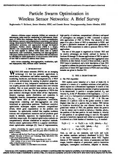
Thus, for a fixed network area A, and a specified data loss fraction Fmax , the ratio of power consumptions depends only on R. The distance R is a measure of the extent to which the path reaches different parts of the network. A dense path (such as a space filling curve) will lead to a small value of R, and therefore significant power savings. If a typical neighborhood WSN has an area A = π(1)2 sq km, and the observer makes use of a local vehicle that carries it to within R = 0.1 km of each sensor, then from (34) we can see that the network communication power is reduced by at least two orders of magnitude (since γ ≥ 2). This comes as no surprise since the required communication range is reduced by a factor of ten. Even from this rough estimate, it is clear that in wide area WSNs, where the communication power constitutes a large percentage of the total power, mobility can aid in reducing communication power considerably. 6.2 Case 2: Disk Network with Circular Closed Path This example evaluates power savings in a disk shaped network with a circular path that is concentric with the network. We will study how power savings change with the radius of the path. Apart for that, this example will also throw light on edge effects and the consequences of a mobility model mismatch. We begin by examining the path itself. A circular path in a circular network may not fit our mobility model in several situations. First, if the radius is small, it will be inaccurate to treat the path as a straight line over distances of the order of the communication range. Second, equation (1) will be valid only if the path is of exactly half the radius as the network. Third, a path with large radius (nearly equal to the network radius) will require a large range to collect data from nodes near the center of the network. This range will be large enough to collect data from points outside the network, or in other words, the network edge will come into picture. But, as we will see, even though the path may not fit our mobility model, it can still save power irrespective of its radius. First, note that the arrival rate will be uniform due to the symmetry of the path, and because the network is dense. Second, since the network is dense, T → 0, and therefore almost all nodes in range will remain in range long enough to receive service. In a dense network, the data rate is given by (29). The choice of communication range is dictated by the requirement that a fraction (1 − Fmax ) of sensors remain within range. This boils down to ensuring that the set of points that are within range Rm from the path of radius Rpath constitute an area (1 − Fmax )A (see Fig. 8). From the above criterion, the minimum Rm necessary for (1 − Fmax )N nodes to be in range is found to be, √ √ 1−Fmax Rnet   1 − Fmax2 Rnet − Rpath 0√≤ Rpath ≤ 2 √ (1−Fmax )Rnet (1+ Fmax ) Rnet 1−Fmax Rnet Rm = < R < path 4Rpath 2 √ 2  √  (1+ Fmax ) Rnet Rpath − Fmax Rnet ≤ R ≤ R path net 2

Using the above, we plot the mobile observer network power (normalized with the static observer network power) corresponding to Fmax = 0.2 for different Rpath and γ in Fig. 9. The plot reiterates that power savings depend on Rpath . As Rpath increases from zero, the range Rm necessary to cover the same area decreases, √ (1+ Fmax ) Rnet thereby saving power. Power savings are maximized when Rpath = . 2 ACM Journal Name, Vol. V, No. N, September 2005.

20

·


Fig. 8. A disk network with a circular path of radius Rpath . Only sensors in the shaded region are able to communicate with the observer O.

For larger values of Rpath , edge effects degrade performance. By edge effect, it is implied that the edge of the network is inside communication range of the observer. When this happens, the observer stops receiving data from some areas that are within range (but outside the network). In other words, a longer range is now necessary to receive data from the same number of sensors, leading to increased power consumption.

Fig. 9.

Role of R in determining power savings

7. CONCLUSIONS AND FUTURE WORK We have demonstrated the feasibility of using a mobile observer to save communication power in a WSN. Not only does the use of a mobile observer save overall network power, it also equates the power consumption at different nodes, thereby ensuring that the network does not become inefficient through localized node failures. There are certain challenges in using a mobile observer that need to be studied further. We have explored the case of a mobile observer that moves on a predictable route. Extensions to partially predictable mobility patterns need to be explored. ACM Journal Name, Vol. V, No. N, September 2005.


·

21

Other extensions include: having nodes with correlated data, or which collect information at different rates; having multiple mobile observers; using heterogeneous networks where not all nodes are power-limited; and using a combination of mobility and multi-hop communication. Work remains to be done in exploring these and other related extensions of this problem. APPENDIX A. CONDITION FOR GUARANTEEING ZERO DATA LOSS The sufficient condition for ensuring zero data loss with minimum separation of nodes d is derived as follows (see Fig. A(a)). In this proof, we will assume that (5) is satisfied with equality. It is obvious that the proof will also be valid for larger communication ranges (if (5) is a strict inequality). Data transfer from a node to the observer takes time T . If we can ensure that the entry of two nodes into the range of the observer is spaced in time by T , then data loss will not occur. Thus, d (see Fig. A(a)), then no other if a sensor node is placed anywhere on the arc AB node can lie within the shaded region ABCD. This implies that the minimum separation d must be greater than or equal to the distance from any point on arc d to any other point on the boundary of ABCD i.e., AB d ≥ max(|x − y|);

d y ∈ ABCD . x ∈ AB,

(35)

Let x = U and y = V be the pair for which |x − y| is maximized. Theorem A.1. U = A and V = C (or U = B and V = D) are the pair that maximizes |x − y|.

Proof: The result follows from a series of claims. The claims themselves are almost trivial to prove, therefore for brevity we will omit their proofs here. d Then, the point Claim A.2. Choose and fix an arbitrary point x = P ∈ AB. y = Q ∈ ABCD, for which |P − y| is maximized does not lie on the line segments BC or AD except possibly that Q is one of the end points A,B,C or D. Corollary A.3. Since this claim holds for arbitrary x, it must hold for x = U , d CD}. d the point which achieves the overall maximum. Therefore, V ∈ {AB,

Claim A.4. Choose and fix an arbitrary point x = P ∈ AB. Suppose that the point y = Q ∈ ABCD is the point for which |P − y| is maximized. Then, unless P d |P − Q| < |U − V |. In other words, U ∈ {A, B}. is one of the end points of AB, d for if V were to lie on AB, d by moving horizonCorollary A.5. V lies on CD d one could show that this point is farther tally to the corresponding point on CD, from U than V is.

The problem is therefore reduced to that of finding V from the set of points on d U has been ascertained to be either A or B (which one we choose makes no CD. d difference). Consider the line passing through A and O0 . This line cuts the arc CD if and only if, (2R)2 + (vT )2 > (2Rm )2 ,

(36)


22

·


(a)

(b)

which contradicts (5). The case of interest is when the line passing through A and d This happens when A lies within the circle centered at O0 O0 does not cut CD. and having radius Rmax . We prove the following claim for this situation. d Claim A.6. When the line passing through A and O0 does not cut CD, |A − C| = max(|x − y|);

x ∈ AB, y ∈ ABCD .

(37)

This also proves our original claim that U = A and V = C (or U = B and V = D) are the pair that maximizes |x − y|. 2 This is the result using which we obtain a meaningful relationship between the minimum separation d and our system parameters. Since, p |A − C| = |B − D| = (2R)2 + (vT )2 , (38)

we conclude that

d≥

p (2R)2 + (vT )2

is a sufficient condition to guarantee zero data loss. ACM Journal Name, Vol. V, No. N, September 2005.

(39)


·

23

The above condition is not necessary to avoid data loss, meaning that it may be violated but data may not be lost. However, an interesting point to note is that if this condition is not satisfied, then there exist bad arrangements of sensors that lead to data loss. Fig. A(b) shows one such arrangement of sensors where data loss is unavoidable with p d < (2R)2 + (vT )2 . (40) B. PROOF OF THEOREM 5.1

The following is a sketch of the proof. We know that power is monotonically increasing with Rm as well as D. We will prove this theorem by showing that ∗ (1) Data loss exceeds Fmax if either Rm < Rm or D < D∗ . ∗ (2) Data loss does not exceed Fmax if (Rm , D) = (Rm , D∗ ), where15 q 2 ∗ (1 − Fmax )R(1 + ) + (vT /2)2 , = Rm

(41)

for any given > 0 and for sufficiently large N .

It is easy to see that the data rate D must equal or exceed D∗ for data loss to remain below Fmax . From (2) and (11), we have, D=

(1 − F )Dnet ≥ (1 − F )Dnet ≥ (1 − Fmax )Dnet = D∗ . fb

(42)

Intuitively, (42) means that the rate D at which data is transferred must equal or exceed the rate at which it is collected by the requisite fraction 1 − Fmax of sensors. ∗ It is also easy to see that Rm cannot be less than Rm for the data loss fraction to ∗ be less than Fmax . Assume for a contradiction that Rm < Rm . Then, since Rm does not satisfy (5), from (19) and (1) p the arrivals at the observer are Poisson distributed p 2 − (vT /2)2 /A = N 2 − (vT /2)2 /RT Rm with a mean arrival rate of 2vN Rm cycle . Therefore, p 2 − (vT /2)2 N Rm Tcycle (43) Average number of arrivals per cycle = RTcycle p 2 − (vT /2)2 N Rm = (44) R q
0, (Rm , D) = (Rm , D∗ ) limits data loss to Fmax . The following result will be necessary for this. ∗ For any > 0, if (Rm , D) = (Rm , D∗ ), then,

lim fb = 1.

(47)

N →∞

The above result will be the most crucial link in substantiating our claim in (28). For the sake of continuity, let us assume that (47) holds. Then, observe that, D=

(1 − F (Rm , D))Dnet Dfb ⇒ F (Rm , D) = 1 − fb Dnet ∗ ⇒ F (Rm , D∗ ) = 1 − (1 − Fmax )fb ⇒ lim

N →∞

∗ F (Rm , D∗ )

= Fmax ,

(48) (49) (50)

which completes our proof. Here, (48) follows from (42), (49) from (29), and (50) from (47). It is now time to prove claim (47). Lemma B.1. limN →∞ fb = 1. Proof: We define the following events: E1 . The observer is idle at a randomly chosen instant t. E2 . All sensor arrivals in (−∞, t] have either been serviced completely before t, or they are past their laxity. √ E3 . All sensor arrivals in (t − c/ N , t] have either been serviced completely before t, or they are past their laxity. Here, c is a constant. It should be clear from the definitions, and from the fact that the scheduling policy is non-idling, that E1 = E2 , and E2 ⊆ E3 . Thus, P (E3 ) ≥ P (E2 ) = P (E1 ) = 1 − fb .

(51)

Now, consider the√event E3 . It is easy to see from (22) that the probability that an arrival in √ (t − c/ N , t] will be past its laxity at t is negligibly small, being √ at most O(1/ N ). Therefore, for E3 to be true, (nearly) all arrivals in (t − c/ N , t] must be serviced completely by t. From (2) and (42), the service time per arrival is T =

fb Tcycle Tcycle Dnet = . ND (1 − F )N

(52)

Therefore, the maximum number of arrivals that can be serviced in a period √cN is √ (1 − F )c N c √ . (53) = fb Tcycle NT √ For E3 to be true, the number of arrivals in (t − c/ N, t] must not exceed the number that can be serviced in that period. Hence, c c P (E3 ) ≤ P Number of arrivals in √ ≤ √ . (54) N NT Since the value of Rm we are considering√does not satisfy (5), √ the arrivals will be 2vN R2m −(vT /2)2 N R2m −(vT /2)2 → ∞ as Poisson with a mean arrival rate of = A RTcycle ACM Journal Name, Vol. V, No. N, September 2005.


·

25

N → ∞. In the limit, as the arrival rate becomes large, the Poisson distribution becomes a Normal distribution with the same mean and variance as the Poisson. Thus, e−µ µx (x − µ)2 1 exp − (55) ≈ √ x! 2µ 2πµ p p 2 2 − (vT /2)2 ) c N (Rm Rm − (vT /2)2 N c √ where µ = = . RTcycle RTcycle N As a consequence of this, P (E3 ) ≤ P

c c Number of arrivals in √ ≤ √ N NT

b√c

=

c

NT X e−µ µx x! x=0

1 (x − µ)2 √ dx exp − 2µ 2πµ −∞ √c − µ 1 NT = + erf √ 2 µ √ √ (1−F )c N − c N (R2m −(vT /2)2 ) 1 fb Tcycle RTcycle r √ = + erf , 2 2 2 ≈

Z

√c NT

c

where erf (x) is the function 1 erf (x) = √ 2π

Z

(56)

N (Rm −(vT /2) ) RTcycle

x

t2

e−( 2 ) dt,

(57)

0

so that erf (∞) = 1/2 and erf (−∞) = −1/2. It is easy to see that for Rm = Rm , √ √ c N (R2m −(vT /2)2 ) (1−F )c N − 1 fb Tcycle RTcycle r √ >1+ (58) lim = ∞ N →∞ f 2 2 b c N (Rm −(vT /2) ) RTcycle

= −∞

1 < 1 + . fb

Now, if fb > 1/(1 + ), then all is well and we find that (56) equals 0 so that, 0 ≥ P (E3 ) ≥ P (E2 ) = P (E1 ) = 1 − fb

(59)

⇒ fb = 1.

If, on the other hand, we assume that fb < 1/(1 + ), then we can arrive at a contradiction by showing that F = 0 contrary to our assumption that Fmax > 0. Physically, this would mean that the system is working at higher power than necessary to ensure the specified Fmax , hence this is not the minimum. For √ obtaining such a contradiction, consider an arrival at some arbitrary time t − c/ N . As argued before, the probability that it will be past its laxity at t ACM Journal Name, Vol. V, No. N, September 2005.

26

·


is negligibly small. We will show that this arrival will have received service with probability 1 if fb < (1 − F ), showing that there is no data loss (F = 0). Since the observer acts as a clairvoyant scheduler with perfect knowledge of node arrivals and deadlines, it will outperform any schedule in terms of data loss F . We will show that even with a non-preemptive non-idling LCFS (Last Come First Served) schedule, F = 0 can be achieved. For convenience, we define the following event: √ E4 . The arrival at t − c/ N does not begin to receive service by t. √ Since the schedule is non-idling, the number of arrivals in (t − c/ N , t] must exceed the number of sensors that can be serviced in that period for E4 to be true. Hence, c c P (E4 ) ≤ P Number of arrivals in √ > √ N NT c c = 1 − P Number of arrivals in √ ≤ √ N NT √ √ (1−F )c N − c N 1 fb Tcycle T q √ cycle . (60) ≈ − erf 2 c N Tcycle

If fb < (1 − F ), then (60) evaluates to 0 as N → ∞, so that we have P (E4 ) = 0. Thus, an arbitrary arrival will receive service with probability 1, implying that the data loss fraction F = 0 which disagrees with our assumption that Fmax > 0. 2 REFERENCES Ailawadhi, V. 2002. Mobility issue in hybrid ad hoc wireless sensor networks. PhD Dissertation. Bhattacharya, P. and Ephremides, A. 1989. Optimal scheduling with strict deadlines. IEEE Transactions on Automatic Control, 721–728. Chakrabarti, A., Sabharwal, A., and Aazhang, B. 2003. Using predictable observer mobility for power efficient design of sensor networks. In IPSN. 129–145. Chakrabarti, A., Sabharwal, A., and Aazhang, B. 2004. Multi-hop communication is orderoptimal for homogeneous sensor networks. In IPSN. Diggavi, S., Grossglauser, M., and Tse, D. 2002. Even one-dimensional mobility increases ad hoc wireless capacity. In ISIT. 352. El Gamal, H. 2005. On the scaling laws of dense wireless sensor networks. IEEE Transactions on Information Theory. to appear. Gamal, A. E., Mammen, J., Prabhakar, B., and Shah, D. 2004. Throughput-delay trade-off in wireless networks. In INFOCOM. Gandham, S., Dawande, M., Prakash, R., and Venkatesan, S. 2003. Energy efficient schemes for wireless sensor networks with multiple mobile base stations. In GLOBECOM. 377–381. Grossglauser, M. and Tse, D. 2001. Mobility increases the capacity of ad hoc wireless networks. In INFOCOM. Proceedings. IEEE. Vol. 3. 1360–1369. Gupta, P. and Kumar, P. R. 2000. The capacity of wireless networks. IEEE Transactions on Information Theory, 388–404. Ishwar, P., Kumar, A., and Ramchandran, K. 2003. On distributed sampling in dense sensor networks: a “bit-conservation” principle. In Allerton Conference. invited paper. Kansal, A., Rahimi, M., Kaiser, W. J., Srivastava, M. B., Pottie, G. J., and Estrin, D. 2004. Controlled mobility for sustainable wireless networks. In SECON. Rao, R. and Kesidis, G. 2004. Purposeful mobility for relaying and surveillance in mobile ad hoc sensor networks. IEEE Transactions on Mobile Computing 3, 225–232.



·

27

Shah, R., Roy, S., Jain, S., and Brunette, W. 2003. Data mules: modeling a three-tier architecture for sparse sensor networks. In SNPA. 30–41. Slepian, D. and Wolf, J. 1973. Noiseless coding of correlated information sources. IEEE Transactions on Information Theory, 471–480. Tong, L., Zhao, Q., and Adireddy, S. 2003. Sensor networks with mobile agents. In Military Communications Conference. 688–693. Wu, Q., Rao, N., Barhen, J., Iyenger, S., Vaishnavi, V., Qi, H., and Chakrabarty, K. 2004. On computing mobile agent routes for data fusion in distributed sensor networks. IEEE Transactions on Knowledge and Data Engineering 16, 740–753. Received January 2005;
