Pre-test Estimation and Testing in Econometrics: Recent Developments.

PRE-TEST ESTIMATION AND TESTING IN ECONOMETRICS: RECENT DEVELOPMENTS Judith A. Giles and David E. A. Giles University of Canterbury, New Zealand Abstract. This paper surveys a range of important developments in the area of preliminary-test inference in the context of econometric modelling. Both pre-test estimation and pre-test testing are discussed. Special attention is given to recent contributions and results. These include analyses of pre-test strategies under model mis-specification and generalised regression errors; exact sampling distribution results; and pre-testing inequality constraints on the model’s parameters. In many cases, practical advice is given to assist applied econometricians in appraising the relative merits of pre-testing. It is shown that there are situations where pre-testing can be advantageous in practice Keywords. Preliminary testing, conditional inference, sequential inference, specification analysis.

1. Introduction 1.1. Background discussion

In applied econometrics it is generally apparent that the researcher has undertaken a ‘search’ for the preferred specification of the model, or for the appropriate estimator to use. Sometimes this strategy is made explicit and it may have been undertaken in a systematic way. In other cases there is only a vague impression that the final results are not the only ones that were generated during the course of the analysis. Most economists who use econometric tools are aware that ‘mining’ the data may be distortive in some sense and that the end results may not be what they appear to be. Consider some simple but common examples of this sort of sequential econometric analysis. First, suppose that the following regression model has been fitted to the data by Ordinary Least Squares (OLS): ~i

= Po + PI XI^

+ P2x2i + e;.

Then, to determine the ‘significance’ of x2 in the model, a t-test is conducted. If the usual t-ratio exceeds the tabulated critical value (for the chosen significance level) then xz is deemed to be a ‘significant’ regressor and it is retained in the model. On the other hand, if xz is ‘insignificant’ it is deleted from the model, which is then re-estimated (effectively by Restricted Least Squares (RLS)). So, the final specification of the model depends on the outcome of a prior test and 0950-0804/93/02 0145-53 JOURNAL OF ECONOMIC SURVEYS Vol. 7 , No. 2 0 Basil Blackwell Ltd. 1993, 108 Cowley Rd., Oxford OX4 lJF, UK and 213 Main St, Cambridge, MA 02142, USA.

146

GILES AND GILES

the estimates of the coefficients of the other variables in the model also depend on the outcome of this test. In addition, the properties of any further tests that may be conducted are affected by the way in which the model’s specification was determined. As a second example, consider the estimation of (1) by OLS. Then, suppose the Durbin-Watson statistic is computed to test whether or not the model’s errors are serially independent. If this hypothesis cannot be rejected, the OLS estimates of the coefficients are retained. However, if serial independence is rejected the model is re-estimated (perhaps using the Cochrane-Orcutt (CO) estimator), and different coefficient estimates are obtained. Again, the estimates that are finally reported depend on the outcome of a ‘preliminary test’, and if (for example) one then tests the significance of a regressor in the usual way, the ‘t-statistic’ is no longer t-distributed. Both of these examples are realistic, though they over-simplify the situation because in practice a sequence of such tests might be adopted. However, they capture the essential feature of ‘pre-test’ strategies in econometrics - the choice of estimator, and the final estimates, depend on the outcome of a random event. The probability of choosing OLS or RLS estimation in the first example, or of choosing OLS or CO estimation in the second example, depends on the significance level for the pre-test, as well as on the test’s power. In effect, the estimator that generates the reported estimates is a stochastic mixture of two (in these examples) ‘component’ estimators. In general this Pre-Test Estimator (PTE) will differ from each of its components in the sense that it will have a different sampling distribution, and so generally its bias and precision will also differ. Pre-testing generally affects the sampling properties of the estimators that we use. For instance, in the first example given above the PTE is biased unless P 2 = 0 . These effects are often complicated and depend on the unknown parameters in the model. Pre-test resting is also widely practised in econometrics, and the consequences of such strategies are of considerable interest. In certain rather special cases, two successive econometric tests may be independent. Then, the effect of the first test on the properties of the second can be controlled, and this may have implications for the extent to which there is a pre-test testing ‘problem’. Two further examples may be helpful. Consider a sequence of ‘nested’ models or hypotheses, such as when we take a multiple regression model, we successively delete regressors in such a way that each model in the sequence can be obtained from its predecessor by the deletion of one or more regressors, and we attempt to find the most parsimonious ‘significant’ model specification. It is well known (e.g., Mizon (1977)) that, with such a nesting, the size of the test of restrictions on the coefficients at any stage can be controlled (against the overall maintained hypothesis) if each null is tested against the previously accepted null in the sequence. Without such nesting, size control is not generally possible, and the resulting size distortion is due to the inherent pre-test nature of the analysis. Similarly, if the hypotheses are nested E Basil Blackwell 1993

PRE-TEST ESTIMATION AND TESTING

147

but the researcher tests each successive null against any alternative other than the immediately preceding null, then a pre-test problem arises. Finally, consider the familiar Chow test for the structural stability of a regression coefficient vector. It is well known that the validity of the standard form of this test relies, among other things, on the homoscedasticity of the error variance across the two subsamples. When this assumption is violated, we have a form of the famous Behrens-Fisher problem and alternative approximate tests are available. So, there is a strong motivation to pre-test for homogeneity of the variance prior to conducting the test of primary interest (the test for structural stability). In contrast to the preceding example, however, in this case the form of the second test depends on the outcome of the pre-test. The standard pre-test statistic in this case is an F-ratio, and it is readily shown (e.g., Phillips and McCabe (1983)) that this statistic is independent of the Chow test statistic. Consequently, the true size of the second stage Chow test is the product of the nominal sizes chosen for this test and for the pre-test. Judicious choices of these nominal sizes can be used to control the true second stage size for the Chow test itself, as desired. However, even with this independence there remains a pre-test testing issue as an alternative test would be used only if the pre-test null was rejected. We explain this further in Section 6.1. Typically non-independence of successive test statistics is the norm in sequential hypothesis testing in econometrics, and in these cases there are pre-test testing issues to be addressed, as we shall see in Section 6. Specifically, how are the (true) size and the power of a second test affected by the presence of a pre-test? Although sequential inference alters the properties of estimators and tests, the commonly held view, that pre-testing is intrinsically ‘bad’, need not be true, as we shall see. It should also be emphasised that these effects arise purely because of the introduction of a randomisation process, and not because the same data are being used more than once. Indeed, even if the sample is split and one part is used for preliminary testing and the other part for subsequent estimation, the pre-test effects that we have described still arise. Also, if a sequence of pre-tests is used, the randomisation process becomes increasingly complicated, especially if the various tests are not independent of each other. In such cases it becomes difficult to determine the properties of the resulting estimators. The above examples will be familiar to anyone who has undertaken applied econometric research. Indeed, pre-testing is probably the norm, rather than the exception, in applied econometrics and so it is not surprising that a sizeable literature on this topic has developed. While much of this literature does not attempt to offer prescriptions about what researchers should or should not do in their empirical work, it does provide a considerable amount of information about the likely consequences of pre-testing in econometrics. Accordingly, the recent contributions in this field are of practical interest to many economists, and the purpose of this paper is to highlight some of the major themes that have emerged recently in the pre-testing literature, at least with respect to econometric 0 Basil Blackwell 1993

148

GILES AND GILES

(as distinct from purely statistical) analysis. We also attempt to extract practical recommendations as far as possible to assist applied workers. 1.2. Historical setting

The seminal contribution of Bancroft (1944) can be taken as the starting point for the analysis of pre-testing problems that are of direct interest to economists. Motivated in part by the earlier remarks of Berkson (1942), that there was a need to investigate the statistical properties of sequential estimation strategies, Bancroft analysed two pre-testing problems which set the scene for much of the subsequent work in this field. The first is as follows. Suppose that we draw two independent samples from two Normal populations, each with possibly different variances. These variances can be estimated separately from the respective samples. We can also test for variance homogeneity, and if this hypothesis is accepted then there is good reason to ‘pool’ the two samples and estimate the (common) population variance from the combined data. In particular this ‘pooled’ estimator may be more efficient than one based on a single sample. This suggests a pre-test strategy: test for variance homogeneity and either pool the data, or don’t, according to the outcome of the prior test. Bancroft derived exact analytic expressions for the bias and variance (and hence Mean Squared Error (MSE)) of this PTE, for the case where the pre-test involves a one-sided alternative. For economists, the interest in this result is that it can be translated into a regression problem where one is testing for a specific type of heteroscedasticity of the errors, and pooling subsamples of data prior to estimating the error variance only if the errors are thought to be homoscedastic. This in turn suggests another related pre-test problem to which we return later: after pre-testing for this type of homoscedasticity, what are the sampling properties of the regression coefficient estimator? The second problem considered by Bancroft was explicitly regression oriented, and was essentially that discussed above in relation to equation (1). To reiterate, suppose a regression model with two regressors has been fitted by OLS, and the model is either retained or simplified by deleting one of the regressors, depending on the outcome of a t-test. Bancroft derived an exact analytic expression for the bias of this pre-test estimator. Subsequent authors considered the estimator’s second moment, and extended the analysis to the more realistic case of the multiple regression model. Much of the basic work on pre-test problems of this type, or problems of ‘inference based on conditional specification’, as it was referred to, was undertaken by Bancroft in collaboration with his colleagues and students. Bancroft and Han (1977) provide an annotated bibliography of this early work, though many of the problems considered are not of direct interest to econometricians. A second bibliograply is given by Han et al. (1988). Pre-test problems with an explicit econometric content were taken up subsequently by a series of researchers. In particular, work by Dudley Wallace .

Basil Blackwcll 1993


149

and a series of graduate students at North Carolina State University led to several seminal developments, and helped to raise interest in this field among a number of Japanese researchers. Other path-breaking contributions came from George Judge, Thomas Yancey, Mary Ellen Bock and their associates and students at the University of Illinois, Purdue University, and later at Berkeley. The range of econometric pre-test problems that has now been analysed is extensive, but in many cases they are essentially variants of those first considered by Bancroft (1944). In the next section the key results from the econometrics pre-testing literature are stated and summarized briefly, as a background to a more systematic discussion of the major themes that have emerged recently in research in this field. These are taken up in Sections 3 to 7, and some concluding remarks appear in Section 8. Each sub-section includes some summary comments to assist the reader who is concerned primarily with the practical implications of the results under discussion.

2. Principal results 2.1. Pre-testing linear restrictions in regression

As in the rest of this paper, we concentrate here on ‘conventional’ PTE’s that is, ones whose components are the traditional ones that have been used in applied econometrics. In particular, while recognizing their interest and importance, we do not consider Bayesian or Stein-like PTE’s. For a discussion of these, the reader is referred to Judge and Bock (1978, 1983), Vinod and Ullah (1981) and Judge et al. (1985). Much of the econometrics pre-test literature is based on a natural generalisation of Bancroft’s second problem. This involves the linear multiple regression model, y =X P

+ e; e - N(O ,u2Z)

(2)

where y and e are ( T x 1); X i s ( T x k ) , non-stochastic and of rank k; and is (k X 1). In addition, prior information suggests rn ( < k) exact independent linear constraints on the regression coefficients

RP=r

(3) where R is (rn x k ) , r is (rn x l), and both are known and non-stochastic. We will consider the estimation of both P and u2. Let 6 = RP - r be the error in the prior information. This situation is commonly encountered in applied econometrics, except usually the researcher is uncertain of the accuracy of the prior beliefs. Accordingly, the procedure usually followed in practice is to (pre-)test the validity of the restrictions and if the outcome of the pre-test suggests that they are correct then the model’s parameters are estimated incorporating the restrictions. If the pre-test rejects the prior information then the parameters are estimated from the sample information alone. Prior to considering the properties 0 Basil Blackwell 1993

150

GILES A N D GILES

of such pre-test estimators of /3 and u2 we will briefly review the estimators which ignore the restrictions (the ‘unrestricted’ estimators) and those which assume the restrictions are correct (the ‘restricted’ estimators). The unrestricted OLS (and maximum likelihood) estimator of /3 is well known to be b = S - ’ X ’ y , where S = ( X ’ X ) and b N ( P , u’S-’). Consequently its risk under squared error loss (the sum of the MSE’s of each individual element of b ) is p ( & b ) = E((b - p)‘(b- 0)) = u2tr(S-’).From the Gauss-Markov theorem we know that b is the best linear unbiased estimator (BLUE). It is minimax and, among the class of unbiased estimators, minimizes risk under quadratic loss. A best (minimum variance) quadratic unbiased estimator of u 2 is the usual least squares estimator, given by 5; = ( y - X b ) ’ ( y- X b ) / u , where u = ( T - k), and p ( u 2 , G f ) = 2u4/u. If we allow the estimator of u‘ to be biased then the estimator of u’ with smallest MSE is ah = ( y - X b ) ’ ( y - X b ) / (u + 2), and as long as the OLS residuals are used, its risk is p(u2, ah) = 2 u 4 / ( u+ 2 ) . The = ( y - X b ) ’ ( y - X b ) /T and maximum likelihood estimator of a’ is p ( u 2 ,6 L L ) = (2u + k’)u4/T2. Imposing the restrictions in (3), we estimate /3 by b* = b + S-’R’[ R S ’ R ‘ ] ( r - Rb), which, with D = S-’R’[RS-’R’] - ‘ R S - ’ , has a risk under squared -‘66‘[RS-’R’]-’RS-’). error loss of p(P,b*)=a’tr(S-’ - D ) + tr(S-’R’[RS-’R’] b* is unbiased if and only if the restrictions are correct (6 = 0).Further, as D is at least positive semi-definite, var(b*) 6 var(bi), i = 1 , 2 , ..., k, and within the class of linear estimators of p, b* is BLUE in this case. = ( y - X b * ) ’ ( y- Xb*)/ The corresponding restricted estimators of u2 are ( u + m),u;’ = ( y - X b * ) ’ ( y - Xb*)/(u+ rn + 2), and = ( y - X b * ) ’ ( y- Xb*)/ T. Now ( ( y-Xb * )’(y- Xb*)/u’) - xt’+m ; where ~ the non-centrality parameter, X, defined by X = 6‘ [RS-’R’]-‘6/2u2, is a measure of the validity of the linear restrictions. If the restrictions are true, 6 = 0 and so X = 0. It is straightforward = 2(2X2 + to show that p(u’, urf2)= 2(2X2 + 4X + u + rn)u4/(u + n ~ )p~( u,2 ,)’;a u + rn + 2)u4/(u+ m + 2)’, and p ( u 2 ,u;:) = (2(m+ u + 4X) + (rn - k + 2X)2)u4/T2. Several studies’ have considered the conditions under which the risk of b dominates that of b* and vice versa. These conditions are generally data specific, as the risks depend on X . This limits the generality of any comparisons based on quadratic risk and so to avoid this complication we will, as others have, concentrate on the conditional forecast of y rather than on p itself. This is equivalent to assuming orthonormal regressors (i.e. X ’ X = l k ) in the /3 space. So, though similar conclusions are drawn from comparing the risk functions, the mapping from the conditional mean (or orthonormal regressors) case to that of considering the unweighted risk of estimators of p (i.e. nonorthonormal regressors) is not direct and is significantly more complicated. The risk of Xb, the unrestricted estimator of E ( y ) , is

-

-’

p ( E ( y ) , X b ) = E ( ( X b- X p ) ’ ( X b - X p ) ) = E ( ( b - P ) ’ X ’ X ( b- p ) ) = a2k, (4)

while that of the restricted estimator, Xb*, is p ( E ( y ) , X b * )= u 2 ( k - rn + 2 h ) . 6 Basil Blackwell 1993

(5)


151

Comparing (4) and ( 5 ) we see that the risk of Xb* is less than or equal to that of Xb if X Q m / 2 , as is depicted in Figure 1. Similarly, there is a X-range over which the risk of the restricted estimator of a’ is less than or equal to that of the unrestricted estimator, as is seen in Figure 2. The values of A, A;, ( j = L , M , M L ) for which the risks are equal depend on the estimation method, but it is readily shown that Xj* # m / 2 and so, if the researcher desired the minimum risk estimators of E ( y ) and u2, there will be some X-range over which his strategy should be to use the restricted estimator of u2 but the unrestricted estimator of E ( y ) . This suggests considering a joint risk function for E ( y ) and u’, something which has not been pursued in the literature. We now consider the situation where the researcher undertakes a pre-test of the validity of the restrictions. Traditionally,

Ho:6= o vs H1: 6

#0

is tested using the Wald statistic g = ( ( ~ b - r )[~~-‘~’]-‘(~b-r)v)/(m(y-xb)‘(y-xb)). ’

If No is correct, the test statistic & has a central F distribution with m and v degrees of freedom, F(m,V). If one or more of the restrictions are invalid, & has a non-central F distribution with m and v degrees of freedom and non-centrality parameter X. We reject HO if & > Fpm,V) = c, where the critical value, c, is determined for a given significance level of the test a , by {: dF(m,u)= Pr. (F(m.0) < c) = (1 -a). This is a UMPI size-a test of the validity of the restrictions. If HOis rejected we use the unrestricted estimators of E ( y ) and a’. If g c, we assume the restrictions are correct and use the restricted estimators of E ( y ) and u2. So, the estimators of E ( y ) and u’ actually reported are the PTE’s

c if& c s p = [ s 6 if J G c '

Bancroft's first problem is equivalent to the one described here with an appropriate re-definition of the degrees of freedom. He derives the bias and variance of sf and finds that the bias of s$ is smaller than that of s6 when 6 is close to zero: that range of 4 where the bias of s i is highest. We recall that the always-pool estimator is only unbiased when the variances are equal. Intuitively, Z Basil

Blackwell 1993

157


the pre-test is leading us to follow the correct path when 4 is small - reject the null. From the MSE comparisons Bancroft finds that the pre-test which uses c = 1 results in a MSE equal to or smaller than that of sk for all possible values of 4 - that is, this PTE strictly dominates the never-pool estimator. These estimators are considered further by Toyoda and Wallace (1975). Figure 3 illustrates typical risk functions for sk, s.$ and s$, for various values of c E (0,oo). Note that when c = 0 we always reject the hypothesis and so, p ( d , s$) = p ( a : , sk). Conversely, p(a:, s$) = p ( a : , s i ) when c = 00, so that we always accept the hypothesis. This figure highlights the following points: (a) Comparing equations (14) and (15), there are two possible values of 4, dl and 42, for which p ( a : , s i ) and p(a:,sk) intersect, provided that u1u2 - 4ul - 2uz # 0 (see Toyoda and Wallace (1975)). In any particular case only one of these values, say $1, will lie in the interval (0,1]. If 0 c 4 < c $then ~ sk dominates s i . Intuitively, the variances are so different that the gain in sampling error from the extra degrees of freedom is outweighed by the bias from pooling the (unequal) variances. Alternatively, s; has smaller risk than sk when 41 < 4 < 1. (b) There exist values of c E (0,2) such that s$ strictly dominates sk for all possible values of 9,0 < 4 < 1. Though these particular PTE's do not dominate s2 for all 4, they do so over a wide range of 4. It is only within the neighbourhood of 4 = 1 that the risk of s i is smaller. Ohtani and Toyoda (1978) prove, for a given value of 4 and c E [0,1], that the minimum pre-test risk occurs when c = 1; so sk is inadmissible and specifically, is dominated (at least) by the PTE with c = 1. These features raise the question of an optimal pre-test critical value - we return to this issue in Section 2.3.

0.1

0.0

0.2

0.3

0.4

0.5

0.6

0.7

0.8

4 Figure 3. Relative risk functions for s&, s6, and sb. 0 Basil Blackwell

1993

0.9

1.0

158

GILES AND GILES

2.2.2. Estimation of the coeflcient vector Assuming that

01 = 0 2 = 0,model (12) is

or

y=Xp+e,

e

- N(0,C). +

If the variances are equal we estimate @ from the T I T2 observations and b~ = X ’ X ’ y , which is the usual least squares (and maximum likelihood estimator) of 0,is BLUE. b~ is the always-pool estimator of 0.However, if the variances are unequal, a feasible GLS estimator of 0 is the ‘two-step’ Aitken estimator (2SAE) b~ = [ S l/s :+ &/sf] - ’ [ X i y ~ / s+: X i y z / s f ] .b N is the neverpool estimator of @. The PTE of @ is

The research on this particular pre-test problem has either worked within the framework of the orthonormal model9 or a reparameterized version of the model l o given by:

+

y = x*p* e,

(21)

where X * = X P , /3* = P - ’ p , and P = T x diag((1 + p i ) - ” 2 ) is a non-singular matrix, and p ; are the roots of the polynomial I Xi&/uf - pLXI’Xl/u:I = 0 ( i = 1, ..., k ) . The matrix T is chosen so as to diagonalise XiXl and Xi& simultaneously. Taylor (1978) establishes the finite sample moments of the ith element of the 2SAE within the context of (21). Let this estimator be i = 1,2, ..., k. He shows that 0 ;; is an unbiased estimator of 0; and that under appropriate conditions the 2SAE is consistent and asymptotically efficient. The least squares estimator of @ * is also unbiased, and Taylor shows that neither estimator dominates, in terms of risk, though he concludes that substantial gains can result from using the 2SAE, depending on the values of u1, ZIZ, 4, and p i . 1 1 Greenberg (1980) follows Taylor’s approach and derives the risk of the twosided pre-test estimator, @:/, corresponding to the ith element of bi., for the reparameterized model and where the test statistic is J* rather than J. He shows that ;6; is an unbiased estimator of p;, and that no one estimator, of those evaluated, strictly dominates the others. Nevertheless, the results would seem to favour the 2SAE, unless one had a very strong belief that the variances were equal. Ohtani and Toyoda (1980) derive the risk of the PTE, for the orthonormal model, when the alternative hypothesis is H I : a: > a t . They show that in this situation the 2SAE is inadmissible, as it is dominated by the PTE when the critical value is chosen appropriately. In particular, if one adopts the criterion of minimizing average risk, then the optimal critical value is unity. Mandy (1984)

Os;,

~Z Basil

Blackwell 1993


159

generalizes Ohtani and Toyoda’s analysis to the non-orthonormal case. He shows that if the direction of the alternative hypothesis is correct then the (inequality) PTE that takes this directional information into account is superior, in terms of risk, to the two-sided (equality) PTE analysed by Greenberg (1980). However, of course, if the alternative hypothesis should be H I :af < a$ then the inequality PTE is risk inferior to the equality PTE. Finally, Adjibolosoo (1989, 1990a) suggests that this traditional pre-test procedure may lead the researcher to use the 2SAE when in fact the degree of heteroscedasticity may be such that it is still preferable to use OLS. Consequently, he considers a PTE (the ‘probabilistic heteroscedasticity PTE’) which chooses between b~ and b N according to a measure of the degree of severity of the heteroscedasticity rather than according to the Goldfeld-Quandt J test. Using a Monte Carlo experiment, Adjibolosoo shows first, that this new test is generally more powerful than the J test and secondly, he shows that the probabilistic heteroscedasticity PTE is typically preferable, in terms of MSE, to its traditional Goldfeld-Quandt counterpart. Some of the most important practical implications for the applied researcher who pre-tests for error variance homogeneity in the two-sample case are the following. First, if estimation of the error variance is of direct interest, then there are advantages in pre-testing with a critical value of unity, rather than using simply the ‘never-pool’ or ‘always-pool’ estimators. Second, as far as estimation of the coefficient vector is concerned, the preferred strategy may depend on the form of the alternative hypothesis for the pre-test itself. If this alternative is that the sub-sample variances are unequal, then the use of the 2SAE (without pretesting) seems advisable. On the other hand, if the alternative hypothesis is onesided then pre-testing with a critical value of unity is again a good strategy. 2.3. Another homoscedasticity pre-test estimator of the error variance Several studies examine the problem of estimating the error variance in the classical linear regression model, y = X/3 + e, e N(0,~ ’ Z T ) ,after a preliminary test of Hot a2 = a;, where a f is some known value available from previous experience. The alternative hypothesis, HA, can be one- or two-sided. If we accept HO then we use a8 as our ‘estimator’ of u 2 , while we use 6’ = ( y - X b ) ’ ( y - X b ) / v , the usual least squares estimator of a2, if we reject Ho. The PTE is then:

-

accept (s’, ifif reject Ho a;,

UP=

HO

a

Assuming orthonormal regressors, Yancey et al. (1983) (see also Srivastava (1976)) derive the risk, under squared error loss, of a$ assuming HA : a’ 2 &and also the risk of the PTE, say a*’, which would arise after testing HO:u2 2 a; vs. HA :a2 < a;. They numerically evaluate their exact risk expressions for a 5% significance level and find, of the estimators investigated, that there is no strictly dominating estimator, though when the direction of the hypothesis is correct, the 0 Basil Blackwell 1993

160

GILES AND GILES

risk of a*’ is always equal to or less than the risk of G2. Comparing the risks has of a*’ and a; their results suggest that if ( a 2 / a f E) [0.75,1.25] then smaller risk than d,while the converse is typically the case for other values of (U’/Uf).

Inada (1989) considers the problem of estimating the variance of a normal variate after a pre-test that the variance lies in the neighbourhood of a known value; that is, HO: [a$co < a’ < afco], where co is a known positive constant. He considers two PTE’s, say PT1 and PT2, where if c i ’ < u / a f < ~1 wu if u / a f 2 c l w-’u if u / a f < c;’

a;

9

and wu P T ~ =[w -lu

ifu/af> 1 if u / a ; < 1’

where u = C l = l (Xi- x>’/(n- l), the weight w is a constant such that 0 < w < 1, and CI is an appropriate critical value. Inada derives the risks of PT1 and PT2, and solves for the values of w such that PT, and PT2 are minimax estimators, given the value of CO. He compares these PTE’s with the traditional PTE a;, and shows that it is preferable to use PT1, in small or moderate samples, when HO is in the neighbourhood of being true, but in large samples, the risks of PTl, PT2, and u are virtually indistinguishable. Ohtani (1991b) (see also Ohtani (1991a)) considers the PTE, d2, which arises after testing HO: a2 = u$ vs. HA : u2 > a f , when we use the Stein (1964) estimator of a’, say a:, rather than G2 if we reject Ho. Recall from the discussion in Section 2.1 that a: is itself a PTE, so a+’ is a special type of multi-stage PTE. We discuss this further in Section 7.2. Ohtani shows that if the direction of the prior information is valid, and the size of the pre-test on a2 is chosen appropriately, then a+’ strictly dominates a:.

2.4. The choice of sign$cance level One feature of these pre-test risk functions considered so far is their dependence on the choice of significance level. If the test size is varied, the pre-test risk function changes, and so too do the differences between the risk of the PTE and the risks of its component estimators. A second feature is that for any particular problem, there exists no dominating estimator; in general, the risks of the PTE and its component estimators cross somewhere in the hypothesis error space. As the extent to which the non-sample information is true or false is unknown, these features raise the question: ‘Is there an optimal choice of test size such that the pre-test risk is as close as possible to the smallest that could be achieved?’. Several studies have addressed this issue. Among other things, the answer depends on the pre-test under investigation and the chosen optimality criterion. C Basil Blackwell

1993


161

First, we review those studies which have considered the optimal choice of test size after a pre-test for linear restrictions. From Figure 1 , the minimum risk that could conceivably be achieved, for all X, is given by the boundary traced out by , for X E [ m / 2 , 0 0 by ) the the risk of the restricted estimator for X E [ 0 , r n / 2 ] and risk of the unrestricted estimator.12 So we desire a choice of test size which results in the risk of the PTE being as close as possible to this boundary. As a increases the risk of the PTE moves down (up) toward the risk of the unrestricted estimator to the right (left) of X = m / 2 , and there is a trade-off between the proximities of the pre-test risk and the minimum risk boundary. There are various ways of measuring this distance. One possibility is the criterion of minimax regret. For a given test size, we determine the maximum regret of p ( E ( y ) , X 6 )from the boundary for all A, then solve for the value of the critical value, c, which minimizes the maximum regret. This value of c is the optimal critical value. For the case of a single hypothesis involving a t test, Sawa and Hiromatsu (1973) use this criterion and find an optimum value of c of about 1.8. (See also Farebrother (1975).) For the situation of multiple restrictions, Brook (1972,1976) chooses values of c, say c*, that minimize the maximum regret on either side of X = m / 2 . This is a slight modification of the Sawa and Hiromatsu criterion. For the conditional mean forecast problem (or, when the regressors are orthonormal), Brook finds that c* is generally very close to two, regardless of the degrees of freedom. This result gives some comfort to researchers who traditionally use the 5% significance level: two is an approximate critical value when the degrees of freedom are moderate to high, say greater than 25, and m > 4. The robustness of this result to model mis-specification is considered in Section 3. Another way of defining the optimal critical value is as follows. Instead of searching for the maximum regret for each level of a,we could take into account the regret for each value of X and search for the value of a which minimizes their sum or average. That is, minimize the area between the pre-test risk and the minimum possible risk boundary. This criterion is considered by Toyoda and Wallace (1976), who find that it leads to a critical value of zero (i.e. use the least squares estimator) if the number of restrictions is less than five. For m < 5 < 60, they find that the (non-constant) optimal critical value is smaller than that observed by Brook (1976), and approximately equal to Brook’s values for rn 2 60. Brook (1976) and Toyoda and Wallace (1976) effectively assume a diffuse (non-informative) prior for A. This may be giving too little weight to small A, as the investigator must believe X is in the neighbourhood of zero to be pretesting at all. l 3 Wallace (1977) postulates that with a strong prior on X weighted towards zero, the minimum average risk critical value would be increased. Toyota and Ohtani (1978) extend the analysis of Toyoda and Wallace (1976) to include prior knowledge about X, by assuming a gamma prior density on X which allows one to weight the likely values of the hypothesis error. They find that if more weight is given to values of X around the null hypothesis then the optimal 0 Basil Blackwell 1993

162

GILES AND GILES

critical values do increase from those proposed by Toyoda and Wallace. Nevertheless, typically, their results support the use of test sizes which are larger than the commonly used ones of 1% and 5 % . Brook and Fletcher (1981) extend the analyses of Toyoda and Wallace (1976) and Brook (1976) to the case of multicollinear (non-orthonormal) regressors. Then the optimal critical value depends on the level of multicollinearity. They consider testing HO: P 2 = 0 in y = XIPl + X2P2 + e, under the usual classical assumptions, where 01 is ((k- m )x 1) and PZ is (rn x l), and show that the optimal critical value of the pre-test according to the Toyoda and Wallace average risk criterion can be well approximated by c&= u(m + t - 4 ) / ( m ( u+ 2)), where u = T - k, t = trace(Cz2) and C22 is the (rn x m ) sub-matrix of the (standardised) matrix

When the regressors are orthonormal C22 = I,,,and t = m,but as the columns of X exhibit higher degrees of collinearity then t increases. Brook and Fletcher find CFW to be very accurate, especially for large m and v values, and they show that the optimal critical value of the prior F-test for t < 4 is 0; that is, it is preferable to ignore the prior information. This is analogous to the result found by Toyoda and Wallace (1976). For t 2 4, c& increases with m and u, and it increases as t increases for a given m and u, implying a higher probability of choosing the restricted estimator. Under a minimax regret criterion Brook and Fletcher show that the optimal critical value, for multicollinear X , is well approximated by cB* = (1 + t / m ) . Recall that for orthonormal regressors t = m and so cB* = 2, as found by Brook (1976). cB* depends only on t / m , and not on u, and increases as the relative degree of multicollinearity ( r / m ) increases. Typically these optimal critical values are still substantially higher than those implied by the traditional 1% and 5010 significance levels, and cB* is close to c& for reasonably large m and u. Until recently there has been no research into the choice of an optimal critical value when estimating the error variance after a pre-test for exact linear restrictions. Then, when using the least squares component estimators, the PTE which uses c = 1 strictly dominates the unrestricted estimator and can also strictly dominate the restricted estimator for m < 2. For the latter case there is then no optimal size problem - it is always optimal to pre-test using c = 1 even i f the restrictions are valid. When using the minimum mean squared error component estimators Ohtani (1988a) shows that the PTE using c = v/ ( v + 2) strictly dominates the unrestricted estimator but that there is still a range in the neighbourhood of the null hypothesis where the restricted estimator has smaller risk. Finally, Giles (1990) shows that it is never better to pre-test when using the maximum likelihood components. Giles and Lieberman (1991b) consider the choice of optimal critical value for a pre-test of exact linear restrictions when estimating the regression error variance. They calculate the critical value, c*, according to a minimax regret C Basil Blackwell 1993


163

criterion and show that regardless of which component estimators are used c * is not constant. This contrasts with Brook’s general finding. However, for a given m , k and estimation procedure, c * is relatively constant as u varies. Giles and Lieberman also compare the risk functions of the PTE which uses c* and that which uses the critical value which minimizes the pre-test risk function (c = 1 for the L estimators, c = u / ( u + 2) for the M estimators and c = 0 for the ML estimators). They find that generally the risk of the PTE which uses these latter (easier to apply) critical values is smaller than that which uses the critical value derived from the minimax regret criterion. We now consider the question of the optimal size for a pre-test for homogeneity. Toyoda and Wallace (1975), Hirano (1978), Ohtani and Toyoda (1978) and Bancroft and Han (1983) each investigate this problem when the parameter being estimated is the error variance, a?, while Ohtani and Toyoda (1980) seek an optimal critical value for the PTE of the location vector in the orthonormal model. Toyoda and Wallace base their choice of optimal critical value on the minimum average risk criterion, with a diffuse prior. They prove that the necessary condition for the minimum is attained when c = 1 and they numerically check the sufficiency and the uniqueness of this minimum. They show that this optimal critical value typically implies a type one error ranging from 40 to 60 percent. Relatively high optimal levels of significance are also reported by Hirano (1978). He considers the choice of significance level one should adopt for the pre-test on the basis of minimizing Akaike’s information criterion. A minimax regret criterion is employed by Ohtani and Toyoda (1978). When the alternative hypothesis is one-sided, they find that the optimal critical value depends on the degrees of freedom and varies from about 1.7 to 2.8. This contrasts with the results of Toyoda and Wallace (1975). Bancroft and Han (1983) investigate yet another criterion: relative efficiency , a, and of the PTE to the never-pool estimator. For given values of u1, ~ 2 and a one-sided alternative hypothesis, they numerically solve for the maximum and minimum values of this efficiency. For certain values of a, the PTE strictly dominates the never-pool estimator; and so, they suggest selecting a test size such that maximum efficiency is the largest and minimum efficiency is no less than unity. This procedure should ensure the largest gain in efficiency. Bancroft and Han find that this criterion results in optimal significance levels in the region of 30% to 50%. Ohtani and Toyoda (1980) adopt the criterion of minimizing average relative risk when they seek the optimal critical value of the pre-test for homogeneity, prior to estimating the location vector in the orthonormal model. They consider a one-sided alternative hypothesis and show that the 2SAE is inadmissible, as it is strictly dominated by the PTE with a critical value of unity. Ohtani and Toyoda derive the extrema of the average relative risk function and conclude that the optimal critical value for the pre-test is c* = 1. From these studies we see the influence of the chosen criterion on the proposed optimal test size. Nevertheless, these results suggest optimal values of a that are 0 Basil Blackwell 1993

164

GILES AND GILES

substantially larger than those traditionally used in practice. Further, depending on the criterion adopted, the optimal critical values may vary with the degrees of freedom. There are some clear prescriptions here for the applied economist who adopts pre-test estimation strategies. If the pre-test relates to linear restrictions on the coefficients then one should apply the F-test with a critical value of two if low predictive risk is desired. If attention focuses on estimation of the coefficient vector itself, then the c& and cB* critical value formulae of Brook and Fletcher provide clear guidelines. On the other hand, when estimating the error variance after this same pre-test, it is generally advisable to use a critical value of unity, u / (v + 2), or zero, depending on whether one uses the OLS, minimum MSE, or ML variants of the scale parameter estimator. Finally, if the pre-test is one for variance homogeneity, a critical value of unity seems advisable when estimating the coefficient vector, assuming a one-sided alternative hypothesis.

3. Robustness of pre-test estimators In any econometric application there is some chance of mis-specifying the model. The errors may not obey the usual ‘ideal’ assumptions; some irrelevant regressors may be included in the model, or relevant ones excluded; the error term may be non-Normal, serially correlated, or heteroscedastic; or the functional form of the model may be mis-represented. The traditional pre-testing literature in econometrics is based on the premise that there are no such mis-specifications. No other ‘complications’ are allowed for. Recently, this situation has been rectified, and several studies have considered some of the consequences of pre-testing in the context of models that are already mis-specified in some way. Specifically, models which are incorrectly specified in terms of the regressors or with respect to the error term assumptions have now been analysed. Pre-testing in the context of a model whose functional form is mis-specified has yet to be researched explicitly, though to some extent it is covered implicitly by the omitted-regressors case. 3.1. Mis-specification of the regressors Mis-specification of the regressor matrix in a linear regression model is a common situation. Extraneous regressors may be included in the model, but it is more likely that relevant regressors will be omitted. The latter situation may arise either because of the researcher’s lack of understanding of the underlying theory, or because certain data are unavailable. In the latter case, another type of mis-specification may also arise - a proxy variable may be substituted for the ‘real’ regressor. With this in mind, several authors have reappraised some of the standard pretest estimation strategies, allowing for such model mis-specification. The inclusion of extraneous regressors is easily dealt with. Giles (1986) shows that in this case the risks of the OLS, RLS and pre-test estimators of the regression Q Basil Blackwcll 1993


165

coefficient vector, after a test of exact linear restrictions on this vector, are the same as in the properly specified model except for a simple scaling of the results. Accordingly, there are the usual regions in the parameter space over which the relative dominance of one of these estimators over the others arises, as in Figure 1 . In particular, such pre-testing is never the best of these three strategies, and can be worst. Moreover, the results relating to the optimal choice of pre-test size are unaffected by such a mis-specification. This situation changes fundamentally if relevant regressors are excluded from the regression. Effectively, this possibility and that of including extraneous regressors was first studied by Ohtani (1983). He considered a pre-test for exact restrictions on the regression coefficients when the model includes proxy variables - that is, effectively, relevant regressors are omitted and irrelevant ones are also included in the model. Unaware of this work, Mittelhammer (1984) dealt with the more extreme case of pre-testing in the context of omitted regressors. Measuring performance in terms of squared error predictive risk, he showed that imposing valid restrictions no longer guarantees dominance of RLS over OLS, or of the PTE over OLS! This should be contrasted with result (a) noted in connection with Figure 1 . Further, referring to result (b) associated with that diagram, the region in which the pre-test and OLS predictive risks must cross is unaltered if the model is mis-specified in this way. Finally, as the degree of model mis-specification increases, the OLS, RLS, and pre-test predictive risks are all unbounded, for a given level of hypothesis error. When the model is mis-specified in this way, it is also natural to ask whether or not the optimal choice of pre-test size is affected. Intuitively, one would expect that the omission of relevant regressors would generally affect this choice, given the preceding comments about the effects on the risk functions themselves. Giles, Lieberman and Giles (1992) re-consider Brook’s (1976) result relating to a preliminary test of linear restrictions on the coefficient vector when the regressors are orthonormal. They find that Brook’s minimax regret criterion no longer leads to an optimal critical F-value of approximately two when the model is mis-specified. In fact, the optimal critical value is then sensitive to the degrees of freedom in the problem, and can differ substantially from Brook’s value. Further, for a given number of restrictions and regression degrees of freedom, the optimal choice of pre-test critical value declines, and the optimal pre-test size increases, monotonically as the model becomes increasingly mis-specified. This has the effect of accentuating the other strong result from Brooks’ analysis - the optimal choice of pre-test size in this problem is often much greater than the commonly assigned values such as 5 % or 1% - when relevant regressors are omitted from the model. Giles and Clarke (1989) study the estimation of the regression scale parameter after the same pre-test in the same mis-specified model. Qualitatively, they come to the same conclusions as Mittelhammer in the case of predictive risk. In particular, imposing valid restrictions need not lead to lower risk than if the prior information is ignored or if a pre-test is undertaken. Clearly, there can be serious 0 Basil Blackwell 1993

166

GILES AND GILES

costs in omitting relevant regressors. Giles (1991b) extends the analyses of Mittelhammer (1984) and Giles and Clarke (1989) to cases in which the disturbances are incorrectly assumed to be normal and we have simultaneously omitted relevant regressors. We discuss this study further in the next section. Estimation of the scale parameter in the context of omitted regressors is also considered by Ohtani (1987a), but for a different preliminary test, namely H o :a2 = af vs. HA : a’ # af or HA : a’ > af. He finds that under the one-sided alternative (but not under the two-sided one), there exists a family of PTE’s for o2 which strictly dominate the unrestricted estimator. This dominance is robust to mis-specification through the omission of regressors. He considers a numerical example with u = 20 degrees of freedom, and conjectures that the PTE based on a size of 45% has minimum risk in this dominating family. It is straightforward to show, using the approach of Giles (1991a, b, 1992b), that the optimal such critical value is c = u (regardless of model mis-specification). This implies a pretest size of 45.8% if u = 20. Assuming a one-sided alternative, Giles (1993) extends Ohtani’s (1987a) and Giles’ (1992b) analyses to the testing of homogeneity in the two-sample linear heteroscedasticity model when relevant regressors are omitted from the models for each sample (possibly different regressors) and the disturbances are spherically symmetric. Then the J test for homogeneity is invalid under the null, as its distribution depends on all aspects of the problem, including the degree of mis-specification and the variance mixing distribution. She also shows that the critical values, identified by Giles (1992b) (see the next section) which minimize the pre-test risk in the correctly specified model also hold this property for the mis-specified model. Analogous to Ohtani’s results, there is a family of PTE’s which strictly dominate the never-pool estimator, and also in some cases the always-pool estimator. It is never preferable to always-pool the samples without testing the validity of the null hypothesis, nor is it optimal to ignore the prior information. Ohtani’s (1983) contribution focuses on predictive risk in the context of proxy variables, when the pre-test involves coefficient restrictions. Implicitly, it subsumes the essential pre-test results of Mittelhammer (1984) and Giles (1986). One of Ohtani’s most important results is that the pre-test strategy can have lower risk than both of its component estimators. This is contrary to the situation in the properly specified regression model, as depicted in Figure 1, and it again underscores the point that once we move away from the make-believe world of a properly specified model to the real-life situation of invalid models, our standard textbook results need to be re-assessed. In this context, perhaps the most important lesson for applied econometricians is that extreme care must be taken over the model’s specification. With a mis-specified model it is difficult to offer many helpful prescriptions. 3.2. Non-normal regression errors Our discussion so far has assumed that the regression disturbances are normally distributed, but there is a large literature which suggests that this assumption is 6 Basil Blackwell

1993

167


sometimes unrealistic. In particular, many economic data series exhibit more kurtosis (and hence fatter tails) than the normal distribution. l4 This has obvious implications for the distribution of the regression disturbance term, and accordingly there has been increasing interest in the sampling properties of estimators and test statistics for non-normal disturbances. Many studies have considered this issue and various distributions have been investigated (see, for example, Judge et al. (1985)). Two general forms of non-normality are usually analysed. The first assumes that the errors are dependent but are uncorrelated (for example, multivariate Student-t errors), while the second assumes that the non-normal errors are identically and independently distributed (for example, univariate Student-t). Little work has been undertaken on the investigation of the properties of PTE’s with non-normal disturbances. Assuming particular non-normal distributions, Mehta (1972) and Giles (1992b, 1993) consider the risk, under squared error loss, of estimators of the error variance after a pre-test for homogeneity of the variances in the two-sample linear regression model, while Giles (1991a, b) derives the risk of PTE’s of the prediction vector and of the error variance after a pre-test for exact linear restrictions. Mehta (1972) considers a family of symmetric distributions given by (0+3)/2 a 21 ) - 1 exp( - 4 I ( x - & ) / a ? I 2 / ( 1 + 0 ) ) , which f ( x I 8 1 , a:, P ) = (r[ (P + 3)/21 includes the normal, double exponential and rectangular distributions as special cases. Mehta considers the problem of estimating the scale parameter from a random sample which follows this distribution when we also have a second, independent, random sample which follows the same distribution but with a? different from a;. The interest in this problem to economists was outlined in Section 1.2. Mehta derives the MSE of two PTE’s of at. The first is analogous to the PTE for this problem that was discussed in Section 2.2 - this PTE is a dis-continuous function of the test statistic. He also derives the MSE of a PTE which is a continuous function of the test statistic, and he compares the MSEs of the estimators. For the cases investigated, the qualitative results are the same for all values of P, the non-normality parameter. He suggests that a test size of between 25%-50% be used. The remaining pre-test literature in this area considers that the departure from normality is to the spherically symmetric family of distributions, which includes the multivariate Student4 (Mt) and normal as special cases. Aside from the normal distribution, this family results in dependent uncorrelated disturbances. One particularly strong motivation for considering this family is that a particular subclass, the so-called compound normal family, can be expressed as a variance mixture of normals. That is, f(e) = JT f~(e)f(7)dr, where f(e) is the probability density function (pdf) of e, fN(e) is the pdf of e when e N(O,T~I) and f(7) is the pdf of T supported on [0,-). Non-normal regression disturbances can arise, even if each ei (i = 1, ..., 7‘) is normally distributed, when the variance of ei is itself a random variable. l 5 For example, the Mt distribution arises if 7 is an inverted gamma variate.

-

0 Basil Blackwell 1993

168

GILES AND GILES

Many studies have investigated linear regression models with spherically symmetric disturbances. l6 Of particular relevance to this paper, Box (1952) shows that the null distribution of g, the test statistic for exact linear restrictions, is the same for all members of the spherically symmetric family.” Thomas (1970) derives the non-null distribution of C and shows that it depends on the specific form of the variance mixing distribution. King (1979) extends many of Thomas’ results. In particular, he shows that if a test has an optimal power property for normal disturbances over all possible values of 7’ then it maintains this property when the errors are compound normal. Consequently, is a UMPI size-a test for compound normal disturbances. King also proves that if any function of y (be it a test statistic or an estimator) is invariant to the values taken by T’ when e N(0, 7’17) then the function has the same distribution for the wider class of spherically symmetric distributions (in fact, elliptically symmetric). So, assuming a correctly specified design matrix, the test statistic for homoscedasticity, J , has the same null and non-null distributions under the wider error term assumption (see also Chmielewski (1981b)). Giles (1992b) considers the same pre-test problem as Mehta (1972) (and for instance, Bancroft (1944) and Toyoda and Wallace (1975) under normal errors) when the disturbances follow the compound normal family of elliptically symmetric distributions, but are wrongly assumed to be normal. She derives the risk of the PTE and also broadens the standard assumption that the never-pool variance estimators are based on the least squares principle. Two families of variance mixing distributions are considered for specific illustrations - the inverted gamma density and the gamma density. The former mixture results in the Mt family of densities, while Teichroew (1957) derives the density and distribution functions of a random variable generated from the latter member of the spherically symmetric family. Giles shows that the results are qualitatively invariant to which of these mixing distributions is used and to the choice of estimation method used to form the never-pool estimator. The key results from the Giles (1992b) study are first, that the PTE can strictly dominate both of its component estimators for sufficiently non-normal disturbances. Secondly, it may be preferable to use the maximum likelihood principle to form the never-pool estimators rather than the least squares principle for non-normal disturbances. Finally, she shows that the risk function of the pretest estimator has a minimum when c * = 1 for the least squares component ) the (usual) maximum likelihood component estimators, c* = v1T2/ ( U I T I for estimators, and c * = (UI ( u 2 + 2))/ (vz(u1 + 2)) for the (usual) minimum MSE component estimators. l 8 Giles (1993) extends this analysis to the simultaneous possibility of omitted regressors, as discussed in the previous section. Assuming a correctly specified design matrix, Giles (1991a) derives the risk of PTE’s of the prediction vector and of the error variance after a pre-test for linear restrictions when the disturbances are compound normal. Her study suggests that the risk properties of the PTE of the prediction vector are qualitatively the same for all members of the compound normal family as presented in Section 2.1 for normal disturbances. In particular, pre-testing is never the preferable

-

(C Basil Blackwell I 9 3


169

strategy. This is incorrect. Wong and Giles (1991) show that it is possible for the PTE to dominate both of its component estimators over some of the A-range. The investigations of Wong and Giles for Mt disturbances, suggest first that the existence and magnitude of the dominating region for the PTE depend on the values of m and Y, the degrees of freedom parameter of the Mt distribution. l9 Secondly, their results show that there is no strictly dominating PTE. Giles (1991a) also shows that the wider error distribution assumption can have a substantial impact on the risk function of the estimators of the error variance. She considers the least squares estimators of the error variance” and she shows that the pre-test risk function has extrema when c = 0, 00, and c = 1, so that the PTE can dominate both of its component estimators. In fact, using the Mt distribution to illustrate, she shows that there exists a family of PTE’s with c E (0,1] which strictly dominate the unrestricted estimator for all A, and the PTE using a critical value of unity has the smallest risk of those PTE’s with c E [0,13 for all A. This family of PTE’s also dominates the restricted estimator over part of the A-range, and the numerical evaluations suggest that this will be strict dominance for small values of Y , say Y < 15. The results also suggest that this may occur for normal disturbances if m is small, say, equal to one. Thus, when estimating the error variance, using the least squares estimators, it is never preferable to ignore any linear restrictions on the coefficients. Pre-testing is always preferable, and the optimal pre-test critical value is unity. Further, it is better to pre-test using c = 1 than to impose the restrictions without testing, unless there is a strong belief that the restrictions are valid. Then pre-testing is better only if Y is small (that is, the tails of the marginal distribution of the disturbances are ‘fat’ in relation to normality) or m is small. Giles (1991b) extends the Giles (1991a) study to the omitted variables model. She finds that the results of Mittelhammer (1984) and Giles and Clarke (1989) assuming normal errors carry over to the wider error term assumption. In particular, imposing valid restrictions does not guarantee a reduction in risk if we have omitted relevant regressors. The question of the optimal size of a pre-test for linear restrictions with nonnormal disturbances has received little attention. The evaluations of Giles (1991a) show that Brook’s optimal critical value of two does not extend to all members of the compound normal family, though she offers no alternative critical value. Wong and Giles (1991) consider the extension of the Brook minimax regret criterion to Mt disturbances. They show first, that the optimal critical values are not constant for all values of Y. Secondly, for a given value of v, the optimal critical values are relatively invariant to the degrees of freedom and the number of restrictions. For instance, for Y = 5 the optimal critical value is approximately 2.4, approximately 2.1 when v = 10, and the optimal critical value of 2 suggested by Brook for normal errors holds reasonably well for the case of Mt errors when v 2 20. Wong and Giles also suggest, if Y is unknown, that a researcher could be (practically) content to continue to use Brook’s optimal critical value prescribed for normal errors. 0 Basil Blackwell 1993

170

GILES AND GILES

Further research is obviously required on deriving the properties of PTE’s under non-normal disturbances. In particular, it would be of interest to know whether the observed results extend to the situation of non-normal but identically, independently distributed disturbances. However, from a practical viewpoint it is clear that in the likely event of non-normal disturbances, the prescriptions offered so far may have to be re-examined. 3 . 3 . Other forms of model mis-specijcation

Recent studies of the effects of model mis-specification on the properties of standard pre-test strategies have proved to be most enlightening, in the sense of overturning a number of apparently strong results which in fact rely on a correct model specification for their validity. A final form of mis-specification that has been considered in this context is that of a nonscalar covariance matrix for the regression errors. Given the likelihood of autocorrelated or heteroscedastic errors in practice, it is natural to ask what effects these may have on some of the standard pre-testing results. The only two contributions to date which respond to this question are those of Albertson (1991) and Giles, Giles and Wong (1992a). Albertson considers the estimation of the regression coefficient vector after a pre-test of linear restrictions on the coefficients, and where the researcher fails to take account of the fact that the errors have an arbitrary nonscalar covariance matrix. Exact analytic results are derived for the OLS, RLS and PTE risks under quadratic loss, and these are evaluated for various data sets and for the cases of AR(l), MA(l), AR(4) and heteroscedastic errors. The form of the regressor variables appears to have some bearing on the results, and several interesting points emerge. First, in the case of trended data and positive AR(1) errors, the usual PTE can be strictly dominated by OLS. Second, MA(1) errors have little or no effect on the relative dominance of the estimators. Third, in the case of nontrended data, or negative autocorrelation, pre-testing becomes more attractive relative to OLS estimation as the degree of model mis-specification increases. Accordingly, prior information about the error process is helpful in prescribing an overall strategy, though it should be noted that autocorrelation pre-test testing raises other considerations, as is discussed in Section 6.4. Fourth, AR(4) and heteroscedastic errors affect the properties of the PTE in a less systematic way, though again it is possible for this strategy to be strictly dominated by OLS, something which cannot occur if the model is properly specified. Other work in progress in this area considers the consequences of this type of mis-specification for optimal pre-test size, pre-test estimation of the regression scale parameter, and investigates the implications of simultaneously misspecifying the error term properties and omitting relevant regressors. Giles, Giles and Wong (1992a) consider the robustness of the exact restrictions PTE for the prediction vector in the multiple regression model, to the presence 0 Baal Blackwell 1993


171

of ARCH or GARCH errors. As such an error distribution is typically more leptokurtic than under normality, it is not surprising that the results are qualitatively somewhat similar to those reported by Giles (1991a) in the case of errors which follow multivariate Student-t and certain other compound Normal distributions. In particular, Giles, Giles and Wong find that when the conventional pre-test is applied (based on the assumption of Normal errors), but the disturbances actually follow a sufficiently strong GARCH process, it is possible for the PTE to strictly dominate both of the OLS and RLS estimators in terms of quadratic risk. Again, the intention of both this latter study and that undertaken by Albertson is to base the analysis of pre-test strategies in a more realistic environment, thus making the results more useful to applied econometricians.

4. Pre-testing with inequality restrictions Frequently, we may wish to test the validity of inequality restrictions on the coefficients of a regression model, as opposed to testing exact equality restrictions, as we have discussed so far. For example, after the estimation of a consumption equation we may test whether the marginal propensity to consume is less than unity. Suppose in the classical linear regression model, y = X @+ e, that we have prior information on the coefficient vector which we express as a single inequality constraint, C’P 2 r, where C’ is a (1 x k) known vector and r is a known scalar. The estimator of which ignores the prior constraint is simply the OLS estimator b, while the estimator which includes the non-sample information is the so-called inequality restricted estimator b**. Rather like a PTE, b** comprises two components: if b satisfies the inequality constraint then b** = 6 , but if C’b < r then b** = b*, the equality restricted estimator, b * = b - (x’x)-’c[c‘(x’x)-’cl -‘(C‘b-r). The sampling properties of b** are well known. Zellner (1961) shows that b** is biased and that it has a truncated normal distribution (see also Judge and Takayama (1966)). This implies, for instance, that a standard t-test based on b** can be misleading (Lovell and Prescott (1970)). The superiority of b** relative to b is considered by, for example, Lovell and Prescott (1970), Liew (1976), Judge et a/. (1980), Judge and Yancey (1981, 1986), Thomson (1982), and Thomson and Schmidt (1982). They find that when the direction of the inequality constraint is correct it is preferable, in terms of quadratic risk, to use b** rather than b. Further, if the direction of the Constraint is in fact incorrect then it is still preferable to use b** rather than b in the neighbourhood of Ho, but b has smaller risk than b** for a sufficiently large hypothesis error. These features are evident in Figure 4, which illustrates typical risk functions for this problem. The sampling properties of the estimator of the model’s parameters which results after a pre-test for the validity of HO: C’p 2 r vs. HA : C’P < r have not received much attention. Assuming that u2 is known, Judge et a/. (1980) and 0 Basil Blackwell 1993

172

GILES AND GILES

Judge and Yancey (1981, 1986) derive the exact risk of the PTE defined by: if we reject Ho

(b

b** if we cannot reject Ho; b * * -

b if C'b 2 r b* if C ' b c r '

So, p^ is the unrestricted OLS estimator of 0, 6 , if we reject the validity of the constraint while it is the inequality restricted estimator of 0,b**, if we cannot reject Ho. Figure 4 depicts a typical risk result (under quadratic loss) and shows, in particular, that it is never preferable to pre-test. In fact, pre-testing is sometimes the worst strategy. These results are qualitatively the same as those that we discussed in Section 2.1 with reference to the pre-test for exact linear restrictions. Hasegawa (1989) considers the unknown u2 case and shows that qualitatively there is no change in the results. He also considers some Bayesian estimators and shows that these can be preferable to the classical estimators, in a risk sense. Yancey et al. (1989) and Judge et al. (1990) extend this literature to the multiparameter hypothesis case (see also Judge and Yancey (1986)). They consider the case of two inequality constraints and investigate a number of potential PTE's. Yancey et al. (1989) examine two multivariate inequality PTE's; the first after

L -6

I

1

-5

-4

C'P > r

I

-3

I

-2

I

I

I

I

I

I

I

-1

0

1

2

3

4

5

C'p = r

C'P < r

CONSTRAINT SPECIFICATION ERROR

Figure 4. Relative risk functions for b, b*, b**, and p^. D Basil Blackwell 1993

6


173

a pre-test of H o : R p = r vs. H A : R /> ~ r and the second after a pre-test of Hd: R p 2 r vs. HA :not Hd. They show that neither of the inequality PTE’s strictly dominates the other. The pre-tests examined by Judge et al. (1990) are similar though, unlike Yancey et al. (1989), they consider the same test statistic for each of the hypothesis tests. Judge et al. (1990) find that no one PTE strictly dominates any other and over some parts of the hypothesis error space the equality restricted PTE has smaller risk than the inequality PTE’s. The current literature on inequality pre-testing has considered only the unrealistic situation of a properly specified model. The effects of model misspecifications on the above results have only recentIy begun to receive attention. Wan (1992) extends the analyses of Judge et al. (1980), Judge and Yancey (198 1, 1986), and Hasegawa (1989) to the case of a researcher who unwittingly omits relevant regressors from the design rnatrix.’l Wan shows that the use of valid prior information in an underfitted model does not necessarily guarantee a reduction in risk. This is consistent with the results found for the exact linear restrictions pre-test which we discussed in Section 3.1. He also shows that many of the results of Judge and Yancey carry over qualitatively to the mis-specified case. An exception is the dominance of b by p^ when the direction of the constraint is valid. This need not occur when we have omitted relevant regressors. Given these results there is an obvious question over the choice of an optimal critical value for the pre-test of inequality constraints. Wan (1992) investigates this issue using the Toyoda and Wallace (1976) criterion of minimizing the average relative risk. His results suggest that for the case of testing one inquality restriction we should simply ignore the prior information and use 6 . This result is analogous to that obtained by Toyoda and Wallace (1976) for the pre-test of exact linear restrictions. We can also define a corresponding inequality PTE of the scale parameter. Wan (1992) derives the exact risk of this estimator for both the correctly specified and omitted variables models. He finds that qualitatively many of the results noted in Section 2.1 and Section 3.1 for the estimation of u’ after a pre-test for exact linear restrictions carry over to the pre-test of inequality constraints on the coefficient vector. In particular, he shows that the choices of c which result in stationary points of the risk function of the PTE are identical to those reported by Giles (1990, 1991a,b). Hasegawa (1991) considers the PTE of the coefficient vector when the pre-test relates to the validity of an interval constraint, HO:rl < C’P < r2, where rl and r2 are known scalars. He assumes that the testing procedure is undertaken in two steps. First, we test HOI: C‘p 2 rl vs. HAI:C‘p < rl using the usual standard normal test statistic (assuming u2 is known). If HOIis rejected we use the OLS estimator b as our estimator of 0. If, on the other hand, we cannot reject H o ~we proceed to the second test, HOZ: C’P < 1-2 vs. HAZ: C‘P > r2. If H02 is rejected then b is used as the estimator of 0, while we use the so-called interval constrained least squares estimator 6’ 0 Basil Blackwell 1993

174

GILES AND GILES

if we cannot reject

H02.

This latter estimator is given by:

I

rl if b c rl b+= b i f r l g b ~ r 2 r2 if b > r2.

The properties of this estimator are examined by, for example, Escobar and Skarpness (1986, 1987), and Ohtani (1987d). So, the PTE is

P+ = ( bb+

if we reject HOIor we accept HOIand reject if we accept HOIand accept H02.

H02

Hasegawa derives the risk, under quadratic loss, of 8’ and he also solves for the critical value of the second stage test, given that this test depends on the outcome of the first stage test. He compares the risks of b+ and p+, finding first that neither strictly dominates the other, and secondly that the preference for one estimator over the other depends on the relative width of the interval constraint. In particular, when the distance of the interval constraint increases, b+ dominates 8’ over a wider range.

5. Exact distributions of pre-test estimators As will be apparent from the discussion so far, the main emphasis in the pre-test literature has been on the first two moments of PTE’s. In particular, the literature emphasizes the use of risk under quadratic loss as a measure of estimator performance, and so it focuses on Mean Squared Error and the associated trade-off between estimator bias and precision. Accordingly, the emphasis is on the consequences of pre-testing for point estimation, rather than interval estimation. To deal with the latter important topic we need more information. For example, to determine the effects of pre-testing on the probability content of a confidence interval we need knowledge of the full sampling distribution of the PTE. Given the additional demands that this places on the analysis, it is not surprising that the econometrics literature was virtually silent on this point until quite recently. To date, there appear to be only two exact results and one simulation experiment relating to the full sampling distribution of PTE’s which are of direct interest to econometricians. Fittingly, the exact results relate to the two problems first studied by Bancroft (1944), as discussed in Section 1.2. Giles (1992a) considers the sampling distribution of the estimator of a variance parameter after a preliminary test of variance homogeneity across two Normal populations; and Giles and Srivastava (1993) derive the sampling distribution of the OLS estimator of a coefficient in a two-regressor model after a preliminary t-test of the significance of the other regressor. The first of these problems has an econometric interpretation in terms of the estimation of the error term’s scale after a pre-test for homoscedasticity in a G Basil Blackuell 1993


175

regression model which may be subject to structural change. So, it relates directly to the earlier discussion in Section 2.2.1. Giles (1992a) considers two random samples, ( X u ) N ( p j , a?); j = 1,2. The usual unbiased estimator of a; is sf = l / n j C E i ( X i j - X j ) ’ , where Xj = l / N j Cp!i X i j , and n j = Nj - 1; j = 1,2. The hypothesis under test is HO:a: = af vs. HA: a? > a;. As is well known, the statistic (s:/s:) is F-distributed with nl and n2 degrees of freedom if HOis true. If HO is accepted there is an incentive to pool the samples and estimate a: by s2 = (nls:+ n 2 s : ) / ( n l+ nz), which leads to the following PTE of a?:

-

3;=

[;:

> Fc

if (s!/s:)

, if

(s!/s$)

< Fc

where Fc= Fc(a)is the critical F-value for a significance level of a. The sampling properties of a: differ from those of the ‘never pool’ estimator, s:, and of the ‘always’ pool’ estimator, s2, In particular, 6: is biased in finite samples. Clearly, misleading inferences may be drawn if one constructs confidence intervals centred on 3!, but with limits chosen as if no pre-testing had occurred. To analyse this situation fully, Giles (1992a) derives the full c.d.f. of a!, which is shown to be a rather complicated function of the various parameters of the problem, but it does not depend on the sample values and is easily evaluated numerically. Given such evaluations, the pdf for the pre-test estimator is readily obtained by numerical differentiation, and is found to be uni-modal. Extending earlier related work by Bennett (1956), Giles (1992a) uses these results to examine the extent to which confidence intervals for a! are distorted when they are based on a:, but with the confidence limits (wrongly) determined from the xi, distribution of s! or the xi,+ n2 distribution of s2. It transpires that as long as HOis not too false, confidence intervals based on pre-testing have higher probability content than those based on s:, while they have lower probability content than those based on sz. The converse applies for large departures from the null hypothesis. Substantial departures from the assumed confidence level can arise in practice, so extreme care must be taken in applied work. As with point estimation, the choice of critical value, Feycan crucially affect the results. Interestingly, when the optimal values suggested by Toyoda and Wallace (1975) and Bancroft and Han (1983) are chosen, there are regions of the parameter space for which the pre-test confidence interval for a: has higher probability content than do either of the intervals based on s: or s2. Broadly speaking, similar conclusions emerge with the problem analysed by Giles and Srivastava (1993). They consider the estimation of @I in the model t = l , ..., T

.,~t=@lxlt+&x2t+~t;

where the ut’s are iid N(0, a2), after a pre-test of HO: /3z = 0 vs. HA: 0 2 # 0. Their results extend earlier related work for Normal means by Bennett (1952). The cdf of the PTE B1 is readily evaluated, and its (uni-modal) pdf is again obtained numerically. Using these results to assist in the evaluation of confidence 0 Basil Blackwell 1993

176

GILES AND GILES

limits, results corresponding to those of Giles (1992a) above emerge. It is clear that while pre-testing may affect the true confidence level of an interval estimate either adversely or favourably, only by applying the unrestricted estimator without any prior testing, can we be sure that the true and nominal levels coincide. Monte Carlo simulation results reported by Basmann and Hwang (1988) focus on the effect of certain pre-tests on the location and shape of the sampling distributions of estimators of a simultaneous structural model. More specifically, the pre-testing situation that is considered relates to the application of a likelihood ratio test of the over-identifying restrictions on the parameters prior to estimation of the latter by Two Stage Least Squares (2SLS) or Three Stage Least Squares (3SLS). The Monte Carlo experiment is based on Klein’s Model I of the U.S. economy. Using the Kolmogorov-Smirnov goodness-of-fit test, the authors conclude that the sampling distributions of the PTE’s under consideration are not particularly sensitive to the size of the pre-test itself. The same goodness-of-fit test, and the first four moments of the estimators are used to compare the conditional and marginal distributions of the ZSLS and 3SLS estimators. On the basis of such a limited study it is difficult to offer strong practical recommendations, but one conclusion that emerges is that the pre-test ZSLS estimator is generally superior to the pre-test 3SLS estimator in terms of bias and MSE, but the latter exhibits less skewness than the former. Also, as it seems that the identifiability test statistic is not distributed independently of the restricted structural coefficient estimators, the usual diagnostic statistics such as ‘t-ratios’ and R Zmay be extremely misleading, and one should be aware of this in applied work.

6. Pre-test testing 6.1. Zntroduction The econometrics pre-testing literature has emphasized pre-test estimation, much more than pre-test testing, resulting in something of an imbalance. However, work in progress may soon alter this situation. To some degree, this imbalance has arisen because the properties of many of the PTE’s that we have considered can be established analytically and without resorting to asymptotic approximations, while the properties of their pre-test test counterparts are generally somewhat less tractable. So, there has been a tendency to focus attention on those problems for which exact results are more readily forthcoming. The two pre-test testing examples cited in Section 1.1 exposed the importance of the independence of successive tests if a controllable pre-test situation is to be attained. For instance, the researcher’s ability to control the overall test size in the context of ‘nested’ hypotheses relies on the independence of such tests, if appropriately formulated, and can be established by appealing to Basu’s (1955) c,

Basil Blackwell 1993


177

independence Theorem. Moreover, Anderson (1971, pp. 34-43, 116-134, 270-276) shows, for the case of normal linear models, that such a nested testing procedure is UMP in the class of procedures which fix the probabilities of accepting a less restrictive hypothesis than the true one. Seber (1964) provides some asymptotic justification when nested testing is conducted in the context of nonlinear models. Here, there is no substantive pre-test testing ‘problem’. Parenthetically it is worth noting that this result provides strong justification for testing from the ‘general’ to the ‘specific’ when deciding on a regression specification, and underscores Learner’s (1988) point that most ‘stepwise regression’ routines are probably better described as ‘stepUNWISE’. The second pre-test testing example given in Section 1 . 1 also involves an independence issue, but one of a different sort. Extensions of that independence result to a range of other interesting testing situations involving statistics based on quadratic forms in normal random vectors are considered by Phillips and McCabe (1989). However, even with this independence there remains a pretesting issue. The Chow test would be used only if the null for the pre-test could not be rejected. Otherwise an alternative test, such as a Wald test, for structural stability would be used. So, even with the advantage of statistical independence there remains a pre-test effect of substance in this case - the true size of the twopart test for structural change will differ from the nominal sizes assigned to the Chow test and its alternative, because of the prior test for variance homogeneity. Furthermore, pre-test testing generally involves an element of nonindependence between the ‘component’ test statistics. In such cases, there are immediate effects on the true (as opposed to nominal) sizes of the second and subsequent tests, as well as on their powers. These issues have been considered primarily in the context of three testing situations in the econometrics literature, each of which is considered in turn below. The properties of certain estimators after more than one preliminary test are discussed briefly in Section 7 under the title of ‘multi-stage pre-testing’. if several tests are undertaken simultaneously, rather than sequentially, then one can consider the global or multiple significance level for the collection of tests. A good discussion of this situation is given by Kramer and Sonnberger (1986, pp. 147-154), and we do not pursue it further here.

6.2. Testing the coefficient vector after a pre-test of the error variance Several studies have used exact analytic methods to consider the properties of the test for linear restrictions on the regression model’s coefficient vector, after a pretest of some hypothesis relating in one way or another to the variance of the error term. In this class of problems, the form of the test for linear restrictions depends on the outcome of the pre-test. For instance, Ohtani and Toyoda (1985) consider a pre-test of the form H o :u2 = uf vs. HA :u2 # a t , where u2 is the regression error variance, and uf is a fixed value, supposedly known on the basis of previous experience or analysis. In this case, the test of primary interest (that of linear restrictions on the coefficient vector) is based on the usual F-statistic if 0 Basil Blackwell 1993

178

GILES AND GILES

the pre-test null is rejected, and otherwise on a Chi-square statistic. Ohtani (1987b) extends this analysis to the case where at is unknown, and it is estimated from an ‘auxiliary’ regression; and Ohtani (1987~)considers a closely related problem, one where the model includes a ‘proxy’ regressor, and the main test of linear restrictions is simply one of the significance of the unobservable regressor which is being proxied. In each of these studies, similar results emerge. The true size of the second-stage test can differ substantially from the nominal size of the main test, especially for small degrees of freedom, but this can be corrected by assigning a 25%-30% significance level to the pre-test. Further, the two-stage test can often be more powerful than the single main test, once size correction has been taken into account. Both of these results have obvious implications for applied researchers. Toyoda and Ohtani (1986) and Ohtani and Toyoda (1988) generalize earlier work by Gurland and McCullough (1962) by considering a more familiar testing problem of the type discussed in the second example cited in the Introduction to this section. Specifically, the pre-test is for variance homogeneity (against either a one-sided or two-sided alternative) in a two sample linear regression situation, followed by a Chow test or an alternative test for the structural stability of the coefficient vector across the two samples, depending on whether the first null is accepted or rejected. The first of these two studies employs a modified (approximate) F-test as the alternative to the Chow test, while the second study uses the Wald test. Consistent with the results noted above, it is found that a pretest size of up to 80% may be advisable in order to avoid size distortion in the test for structural change. Then, the two-stage test is generally more powerful than the single stage test suggested by Jayatissa (1977) and the Wald test, though typically less powerful than the size-corrected variant of the latter suggested by Rothenberg (1984). Again, there are some clear implications here for applied econometricians. 6.3. Testing the error variance after a pre-test on the coeficient vector A pre-test testing strategy which is essentially the reverse of the ones just discussed is considered by Ohtani (1988b). Specifically, his pre-test relates to exact linear restrictions on the regression coefficient vector, while the main test of interest is of HO:u2 = a?, against HA :u2 # u;, where at is known. As before, the size of the two-stage test can be controlled to that of the main test if the nominal pre-test size is much larger than would commonly be chosen. Specifically, a size of the order of 30% is recommended. Again, with such a choice, pre-test testing can be more powerful than applying the main test by itself. 6.4. Autocorrelation pre-test testing

In the next section we consider the properties of various estimators involving a preliminary test for the serial independence of the regression errors. However, @ BasilIBlackwell 1993


179

autocorrelation pre-testing also gives rise to some important pre-test testing situations. Primarily, attention has focused here on the following problem what are the properties of the usual t-test for the significance of a regression coefficient after a prior Durbin-Watson (or similar) test for autocorrelation? In this case, the form of the ‘t-test’ varies according to the outcome of the pre-test - if the null of independent errors is accepted then the t-test is based on OLS estimates; but if the errors are found to be autocorrelated then the second test is based on Cochrane-Orcutt or full maximum likelihood estimates, for example. Attention has centred on tests of single linear restrictions at the second stage, and the nature of the problem has necessitated Monte Carlo simulation rather than exact analytical treatment. Nakamura and Nakamura (1978) and King and Giles (1984) have studied this problem. The former study is the more limited, being based on a model with a single trended regressor, and considering only the Durbin-Watson and Geary autocorrelation tests. A much wider range of tests and design matrices are examined by King and Giles, and (following the findings of Fomby and Guilkey (1978)) both 5% and 50% sizes are considered for the pre-tests. Nakamura and Nakamura find that the size of the pre-test ‘t-test’ exceeds its nominal size, increasingly so as the degree of positive first-order autocorrelation in the errors increases. They also suggest that simply adjusting for autocorrelation and then testing is preferable to either pre-test testing, or t-testing on the basis of OLS estimation in this context. This preference is based on the degree of size distortion. King and Giles find that their results are somewhat sensitive to the regressor data, and that trended regressors can produce extreme results, so this raises some questions as to the strength of the results just cited. Generally, they find that the size of the pre-test ‘t-test’ is distorted less than those of the two component ‘t-tests’, especially if a 50% pre-test size is used. Further, once size distortion is taken into account, the powers of the pre-test ‘t-test’ and the ‘t-test’ conducted after an automatic allowance for AR(1) errors are found to be similar, and greater than that of the simple OLS-based t-test. These results are quite supportive of autocorrelation pre-testing, especially if a larger than usual pre-test size is adopted, and they are broadly consistent with the principal results discussed in the last two subsections. The converse autocorrelation pre-testing problem is discussed by Giles and Lieberman (1992). That is, they consider the size and power of the (exact) Durbin-Watson test after a preliminary t-test. Their results are based on a mixture of analytical and Monte Carlo results. When there is no pre-testing the exact power properties of the Durbin-Watson test are easily computed for any regressor data, but a simulation experiment is needed to analyse the pre-test strategy. Working with a range of data sets, different sample sizes, and pre-test sizes of 5 % and 50070, Giles and Lieberman find that pre-testing distorts the true size of the Durbin-Watson test above its nominal value, unless the restriction under test is true. This distortion can be reduced in percentage terms by choosing a large nominal size (say, 50%) for the Durbin-Watson test, The results with respect to 0 Basil Blackwell 1993

180

GILES A N D GILES

power are less clear, but there are situations in which pre-testing can result in increased power for the Durbin-Watson test. These results suggest that autocorrelation pre-testing, defined in either of the above ways, is not necessarily a ‘bad’ thing. Moreover, they lend considerable support to the case made by Fomby and Guilkey (1978)for assigning much larger sizes than usual to tests for autocorrelation, and this should be borne in mind by applied econometricians. 7. Other developments

There are several other important pre-test problems which have attracted attention in the more recent econometrics literature. Some of these are discussed briefly in this section.

7.1. Autocorrelation pre-test estimation The second motivating example given in Section 1.1 serves as an introduction to an interesting pre-test situation that arises frequently in applied econometrics. That example relates to the use of the Durbin-Watson test for serial independence of the regression errors, as a basis for choosing between least squares estimation and Cochrane-Orcutt estimation of the regression coefficients. Pre-test strategies of this general type have been analysed to some degree. Judge and Bock (1978,pp. 143-164) consider the empirical risks of such autocorrelation PTE’s based on both the Durbin-Watson and Berenblutt and Webb tests, with various component estimators. Specifically, the Durbin, Cochrane-Orcutt and Prais- Winsten estimators are considered when a positive AR(1) error process is detected by one of the tests. A limited Monte Carlo experiment, based on a model with four orthonormal regressors, forms the basis of their analysis, and estimator performance is measured in terms of risk under squared error loss. Only positive autocorrelation is considered. The risks of the component estimators and of the various PTE’s increase with the degree of autocorrelation. This study suggests, among other things, that it is the choice of estimators, rather than the choice of test, which determines the risk consequences of autocorrelation pre-testing. Strategies which incorporate the Durbin estimator when serial correlation is detected are especially favoured. It also indicates that autocorrelation pre-testing doesn’t incur particularly large risk losses (relative to no pre-testing), even when there is slight serial correlation, and for moderate to large degrees of serial correlation there can be substantial gains from pre-testing. These conclusions are corroborated in recent work by Chen and Saleh (1991). Their experimental design is virtually identical to that of Judge and Bock, but they emphasise the performance of autocorrelation pre-test strategies based on shrinkage estimators of the type proposed by Sen 2nd SaM (1985) and Saleh a d Sen (1985). In particular, they find that autocorrelation PTE’s of this type E Basil

Blackwell 1993


181

uniformly dominate their conventional autocorrelation pre-test counterparts. This illustrates the (known) inadmissibility of standard autocorrelation pre-test strategies, in the same way that Judge and Bock (1978, pp. 189-195) illustrate the inadmissibility of the conventional linear restrictions PTE for the regression coefficients. (Of course, the autocorrelation PTE’s suggested by Chen and Saleh are themselves inadmissible, being discontinuous functions of the random data.) King and Giles (1984) extend the results of Judge and Bock in several directions by considering additional tests for serial independence as well as the full maximum likelihood estimator to allow for AR(1) errors. They also consider the effects of autocorrelation pre-testing on the power of the test for regressor significance, as was discussed in Section 6 above, and on predictive performance. Their Monte Carlo experiment is more comprehensive than those discussed above, with an allowance for different (nonorthogonal) design matrices with three to six regressors, different sample sizes, and both the 5% and 50% pre-test significance levels. The latter size reflects results obtained by Fomby and Guilkey (1978), and extended recently by Kennedy and Simons (1991). Fomby and Guilkey showed that, in terms of maximizing the (MSE) efficiency of the PTE relative to that of OLS, after a preliminary Durbin-Watson test, the size of the latter test should be of the order of 50%, rather than the conventional 1% or 5%. One of the most important findings from the study by King and Giles is that the form of the regressor matrix is crucial in determining the risks of autocorrelation PTE’s. This implies that other related results based on more limited studies should be interpreted cautiously. This study also finds that PTE’s which incorporate the full maximum likelihood estimator to allow for autocorrelation are preferable to those which involve the Durbin estimator, except for problems involving relatively small degrees of freedom. At conventional significance levels, and especially with small sample sizes, the results also suggest a slight preference for the Berenblutt and Webb test, or King’s point optimal test as the pre-test. The choice of pre-test is generally less consequential if a 50% significance level is used. Griffiths and Beesley (1984) extend the earlier Judge-Bock analysis in a different direction. In a Monte Carlo experiment limited to a single regressor model, but considering both trended and stationary data, they analyse the autocorrelation PTE based on the (two-sided) Durbin-Watson test and either OLS or Maximum Likelihood estimation. They also consider what is effectively a multi-step PTE (further examples of which appear in the next subsection). In particular, they analyse the consequences of using the Durbin-Watson test to discriminate between serial independence and autocorrelation of the errors, and Akaike’s Information Criterion to select between AR( 1) and MA( 1) disturbances in the latter case. In terms of reasonably uniform point estimation relative efficiency over the entire parameter space, the multi-step PTE is found to be quite successful. However, in the case of interval estimation, the OLS-AR(1) PTE of the form considered by the other authors is found to be preferable to multistage pre-testing, at least in terms of the tests considered by Griffiths and 0 Basil Blackwell 1993

182

GILES AND GILES

Beesley. As with the results of King and Giles, the type of regressor data is found to be an important determinant of the estimators’ relative performances. Folmer (1988) provides a more complete summary of the studies discussed above, and provides Monte Carlo and bootstrap approximations to the full distribution of the autocorrelation PTE based on the Durbin-Watson test and the OLS and Durbin estimators. His results accord with those noted already, and he concludes that (wrongly) applying standard results, when autocorrelation pretesting has taken place, can be very misleading. This is especially so in the case of confidence intervals, a result which accords with the conclusions reached in Section 5 above. Autocorrelation pre-testing in the context of models which include a lagged dependent variable as a regressor is considered by Giles and Beattie (1987). Again, given the nature of the problem, this study is based on Monte Carlo analysis. The risks of nine PTE’s are evaluated, and are found to exhibit similar shapes to those encountered in the fixed-regressor studies discussed already. Consistent with those other results, this study also finds that autocorrelation pretesting can lead to significant reductions in risk over large parts of the parameter space, and that the choice of component estimators is generally more important than the choice of preliminary test. PTE’s which incorporate Wallis’s (1967) three-step procedure and Durbin’s (1970) ‘rn test’ are found to be advantageous from a risk viewpoint. In summary, autocorrelation pre-testing is generally preferable to simply applying OLS. In terms of both point estimation and interval estimation, pretesting is also preferable to simply estimating under the assumption of AR(1) errors when the degree of autocorrelation is small, and for high degrees of autocorrelation pre-testing is no worse than this alternative approach. Finally, significance levels much higher than those conventionally assigned in econometric work deserve serious consideration in this context. 7.2. Multi-stage pre-testing

Though the majority of the pre-test literature concentrates on the properties of PTE’s after a single pre-test, the analysis of multi-stage PTE’s has recently received attention. This is, of course, closer to the procedure actually undertaken by applied researchers, who would typically undertake a series of pre-tests prior to deciding the ‘final’ version of the model. For instance, a researcher may test for autocorrelation, and on the basis of this test decide whether to use OLS or some feasible GLS estimator. After this decision, he may then undertake a test for heteroscedasticity, with the test used being dependent on the outcome of the prior pre-test for autocorrelation. The outcome of the second pre-test - the heteroscedasticity test - will determine whether he keeps the ‘current’ version of the model or whether some modification is undertaken and so on. Clearly, given that each step in this sequential testing procedure is dependent on the outcome of the previous pre-test, and that typically the tests are not independent of each other, it is difficult to derive the properties of multi-stage @Basil . Blackwell 1993


183

PTE’s analytically. To date, as far as we are aware, only four studies have attempted to consider some finite sample properties of various multi-stage PTE’s - Shukla (1979), Adjibolosoo (1990b), Ozcam and Judge (1991), and Ohtani (1991a). Shukla (1979) considers the estimation of the slope coefficients in the twosample simple linear regression model yij = * / j + Pjxij + eij;

j = 1,2; i = 1,2,..., Tj;

-

where eij N(0, a’), after two preliminary tests of significance. The first pre-test is of HoI:u’=a,; where a; is a known constant, and this test is undertaken using a Xz-statistic. The second pre-test is of HOZ:PZ= 01, for which a z-test is used if we do not reject H O Iwhile , if we reject HOIa t-test is undertaken. Shukla derives the bias and MSE of the PTE of PI. Unfortunately, though he notes that the expressions are too complicated for comparisons to be made, he does not undertake any numerical evaluations of the expressions. Ozcam and Judge (1991) extend Shukla’s investigation to the multiple regression case and possibly heteroscedastic error variances. The first pre-test is of HOI: af = af (vs. HAI:a: > a t ) followed by a second pre-test of H 0 2 : PI = PZ (vs. H A Z PI : # Pz) in

-

where ei N(0, afI~,) and the usual assumptions on Xi are satisfied; i = 1,2. The two-stage pre-test estimator (2SPE) of 61, assuming orthonormal regressors, comprises the least squares estimator (LSE = (Xfyl + Xiy2)/2), the Two-step Aitken estimator (2SAE = (Oxiyl + (1 - O)Xiyz), where O=s$/(sf+sf) and sf is the usual unbiased estimator of a;) and the Gauss-Markov estimator (GME = Xiyl). HOI is tested using the Goldfeld-Quandt test, while HOZis tested using the Chow test if we accept that the error variances are homoscedastic, but using the Wald test if we reject homoscedasticity. Ozcam and Judge derive the risk, under quadratic loss, of the 2SPE and using numerical evaluations of these exact expressions, they compare the estimators assuming that each test is undertaken at the (nominal) 5% level. For a given value of a$at they find that the 2SPE is preferable to the GME, regardless of whether 61 and PZare equal. Further, their results suggest that the risk advantage of the 2SAE and the LSE over the 2SPE under HOIdisappears as the difference between 01 and PZ disappears. Adjibolosoo (1990b) also considers a two-step estimator of the coefficients in the two-sample heteroscedastic linear regression model. Following the lines of Adjibolosoo (1989, 1990a) he considers the possibility that one may still prefer to use the LSE even if HOIis rejected, if the degree of heteroscedasticity is not severe, and suggests that a second step should be incorporated if we reject HOI to compare the relative efficiency (strong MSE) of the LSE and the 2SAE. If the LSE is relatively more efficient we use this estimator even though we have rejected homoscedasticity. Using a Monte Carlo experiment, he shows that the 0 Basil Blackwell 1993

184

GILES AND GILES

risk of the two-step PTE is typically better than that of the traditional PTE discussed in Section 2.2.2. Ohtani (1991a) investigates the sampling properties of a PTE for the variance of the classical linear regression model, a+’, after a pre-test for homogeneity H O Za’: = af,where ui is known (vs. HAI: a’ > af)when the estimator we use if we reject the null hypothesis is Stein’s (1964) estimator, .:a We mentioned Ohtani’s study in Section 2.3 and we recall that a3 is itself a PTE with its and unrestricted (ah) minimum MSE components being the restricted (a;’) estimators of the error variance when the test critical value is u/ ( u + 2). The pretest is for exact linear restrictions, Ho, :RP = r vs HAL:RP # r. So, we first test HOIusing a critical value of v/ (u + 2); if we reject this hypothesis we use & while we use a$’ if we accept H O I .Thus, the estimator actually used is a.: We then test HOZ;if we accept HOZwe use uf,while we continue to use a: if we reject HOZ. Ohtani derives the MSE of this two-stage PTE and compares it with that of a: using numerical evaluations. He shows that if the size of the test for HOZis chosen appropriately (say, 25%) then the two-stage PTE strictly dominates the Stein estimator, assuming that the direction of HAZis valid, and that it is only around the neighbourhood of HOZbeing true that other choices of test size may be more appropriate. Given these studies, it is apparent that further research is required into the properties of multi-stage PTE’s. Nevertheless, the papers discussed in this section suggest that multi-step pre-testing may be a preferable option to naively imposing or ignoring prior information. 7.3. Alternative loss functions

All of the above discussion reflects the emphasis in the econometrics pre-testing literature on the use of a quadratic loss function. The appeal of this type of loss, of course, is that it leads to risk measures which are in the form of matrix MSE (or its trace), and so incorporate the familiar bias-variance tradeoff when assessing estimator performance. However, an interesting question that naturally arises is, ‘to what extent are the various results in the pre-testing literature robust to departures from the quadratic loss assumption?’ There is only scant evidence in answer to this question, though this is an important topic currently under research. One feature of a quadratic loss function is that it is symmetric - underestimation and overestimation are equally penalized. Accordingly, it would be interesting to know whether the standard pre-testing results are sensitive to choices of loss functions which are nonquadratic, but still symmetric, as opposed to ones which are asymmetric. With respect to the former, there is apparently no published evidence. Work by Giles (1992~)reconsiders the first of Bancroft’s (1944) problems in terms of risk based on an absolute error loss function. The results suggest that, except in one respect, the known results under quadratic loss apply qualitatively under absolute error loss. In particular, when estimating a single regression coefficient after a preliminary t-test of the significance of the second regressor, the risk of the @ Basil Blackwell 1993


185

unrestricted estimator is still independent of the test statistic’s noncentrality parameter; the pre-test estimator’s risk has the same shape properties as in Figure 1; but the risk of the restricted estimator is mildly concave to the origin. The same types of regions of estimator dominance hold as for the quadratic loss function. So, pre-testing can be the worst strategy, it is never best, and the usual question of the optimal choice of pre-test size arises. Any symmetric loss function is unduly restrictive in certain estimation situations. For example, underprediction and overprediction of the future exchange rate are unlikely to be equally costly mistakes. Underestimating the error variance in a regression model will lead to calculated t-statistics which make the regressors appear to be more ‘significant’ than is warranted. A conservative researcher may prefer to err in the opposite direction. Work in progress by Giles, Giles and Wallace (1992) considers the former problem, using the asymmetric LINEX loss function proposed by Varian (1975), and subsequently adopted by Zellner (1986) and Srivastava and Rao (1992). Using this same loss function, of which quadratic loss is a special case, Giles and Giles (1993a,b) consider the second problem suggested above. They consider the estimation of the scale parameter in a multiple regression model with Normal errors after a preliminary test of exact linear restrictions on the coefficient vector, or after a pre-test of variance homogeneity. They find that the risk functions for the pre-test, unrestricted, and restricted estimators are robust to mild departures from quadratic loss (at least qualitatively). However, as the degree of asymmetry in the loss function increases, rather different results can emerge. On the basis of this limited information, it seems that the PTE properties may be reasonably robust to departures from quadratic loss which are still symmetric, or only mildly asymmetric. Strong asymmetry in the loss function, however, may lead to results at variance with those in the established literature, and this remains a topic for further investigation. 7.4. Other pre-test problems

As we have seen already, many of the tests that are used in econometrics can be reduced to ones of the validity of exact restrictions on the regression coefficients, or to tests that can be linked to homoscedasticity of the regression errors. Accordingly, the detailed attention that we have paid to the related PTE’s effectively covers a range of specific situations, such as testing the ‘significance’ of an individual regressor, or testing for structural change. Also, there are other closely related pre-test situations that are of interest to economists. One recent such example is the problem of estimating the regression coefficient vector after a linear restrictions pre-test, but in a situation where there are two sets of linear constraints, one of which contains only valid information, but the second of which may contain some invalid information. This problem is studied by Hessenius and Trenkler (undated), who derive necessary and sufficient conditions for the dominance of the PTE in terms of matrix MSE.” Another example, considered by Griffiths and Judge (1989), involves 0 Basil Blackwell 1993

186

GILES AND GILES

estimating regression coefficients after the application of Weerahandi’s (1987) test of coefficient stability. This test allows for the possibility that the errors may be heteroscedastic across the two sub-samples. The component estimators in this case are OLS and the restricted 2SAE. Using Monte Carlo analysis, Griffiths and Judge compare this PTE with the corresponding one based on an asymptotic Ftest23and find that although the former PTE is slightly risk-superior to the latter for small degrees of hypothesis error, generally there is no clear advantage in using Weerahandi’s ‘exact’ test, rather than the asymptotic F-test, in this pre-test environment. There are other interesting pre-test problems of various sorts which deserve brief mention here. For example, Morey (1984) derives the asymptotic risks of specification pre-test estimators based on Wu-Hausman tests in the context of a linear model which may be mis-specified in the sense that certain of the errors may be correlated with the disturbances. The two component parts of this PTE for the coefficients are OLS (if the test suggests independence between the errors and the regressors) and Instrumental Variables (IV) estimation (if the errors and regressors are thought to be correlated). The most interesting feature of Morey’s results is that this PTE is strictly dominated by the IV estimator itself. However, to be conservative, and given that the degree of mis-specification will be unknown in practice, Morey recommends against simply using the IV estimator without a pre-test, and instead suggests testing with a much higher significance level than would usually be adopted. In this respect his results accord with those discussed already in the context of autocorrelation pre-testing. More recently, Ozcam et al. (1991) consider an important PTE in the context of the Seemingly Unrelated Regressions (SUR) model. The setting for their analysis is a two-equation SUR model with orthonormal regressors, and the PTE is based on OLS and GLS, depending on whether there is evidence of crossequation (population) correlation between the disturbances. The latter is tested using the corresponding sample correlation coefficient based on the ‘restricted’ OLS residuals. Although the (squared error) risks of the PTE and its components ‘cross’ in the usual sense, there are regions of the parameter space over which the PTE’s risk is the smallest of the three. As we have seen already, contrary to popular mythology (which is based on the standard ‘exact restrictions’ PTE problem) there are situations in which pre-testing can be advantageous from a MSE viewpoint. The pre-test literature has not kept pace fully with certain significant developments in econometrics which are of vital importance to applications in both macroeconomics and financial economics. The modelling of high frequency financial time-series now invariably considers the possibility of leptokurtic errors, specifically by specifying some sort of autoregressive conditionally heteroscedastic (ARCH) process for the disturbances. Very little is known about the properties of pre-test strategies in the context of ARCH or GARCH regression errors. The nature of the problem does not allow an analytical treatment, and finite-sample results must be obtained by Monte Carlo simulation. Q Basil Blackwell 1993


187

Engle et al. (1985) consider the following pre-test problem. The model is estimated by OLS and a one-sided version of the LM test for ARCH(]) errors is applied in its nR2 form. Depending on the outcome of the test, either the OLS results are retained, or the coefficients are re-estimated by MLE. This PTE is found to be unbiased. Moreover, in terms of finite sample efficiency, it is found to be little worse than OLS when the errors are free of an ARCH process, much better than OLS when there is an ARCH effect present, and almost as good as the MLE in the latter case. Giles, Giles and Wong (1992b) consider a related pretest testing problem. They use Monte Carlo analysis to determine the effects that various pre-tests for ARCH(p) or GARCH(p,q) errors have on the size of a subsequent ‘t-test’ for the significance of a regressor. Their results show that such pre-testing is quite innocuous in samples of 100 or more observations, but in small samples it may be preferable to use a smaller than usual size for the pre-test. Empirical macroeconomics has been revolutionized in recent years with the recognition that the use of cointegrated time-series has special implications for model formulation, estimation and testing. Several tests for the order of integration of time-series, and for their possible cointegration, are now routinely used. Pre-test strategies also abound in this context in practice, though their implications are only just beginning to be explored. Again, the asymptotic nature of the tests concerned necessitates the use of Monte Carlo simulation to analyse the finite-sample properties of cointegration pre-test estimators and tests. This remains a fruitful and important area for research, and work underway by the authors 24 considers such issues as the effects that multi-stage sequential pretesting for order of integration and the presence of cointegration may have on test sizes; and the finite-sample properties of estimators of the parameters of VAR/error correction models after cointegration pre-testing.

8. Conclusions In this paper we have attempted to provide an overview of preliminary-test problems as they arise in econometrics, and to indicate some of the recent developments in this field. Inevitably, there will be omissions, but hopefully we will have captured the principal thrust of the associated literature while exposing both the historical and recent connections between the different strands of research into pre-testing problems. A number of specific practical implications that arise from the econometric pre-testing literature have been presented in the paper. However, by way of conclusion it may be appropriate to offer some general comments. First, pre-test estimation and pre-test testing are perhaps the norm rather than the exception in applied econometric analysis, so the issues and results that we have discussed are of direct relevance to economists who engage in empirical work. Second, once pre-testing takes place the standard ‘textbook results’ relating to the properties of various estimators and tests generally no longer apply. For instance, estimators which are unbiased under a specified set of assumptions or 0 Basil Blackwcll 1993

188

GILES AND GILES

conditions may be biased if used after one or more preliminary tests relating to the specification of the model. The applied researcher should be aware of this as it may affect the overall strategy that is adopted when specifying, testing and estimating an economic relationship. Third, and contrary to a commonly encountered viewpoint, this is not to say that pre-testing is necessarily a ‘bad’ thing. On the contrary, we have given examples of situations in which pre-testing may lead to estimators which have uniformly smaller Mean Squared Error than can be achieved by applying the estimator without a suitable prior test. The essential point is that the sampling properties (such as bias, efficiency, size and power) of the estimators and tests that economists use in their empirical research are typically altered if pre-testing occurs prior to their application. Fourth, as with any estimators or tests, the established results are based on various assumptions, including the presumption that the model is ‘correctly specified’. If any of these assumptions are violated then typically the established results are affected. One of the recent developments in the pre-testing literature has been an examination of the robustness of established results to the type of assumption violations (such as the omission of regressors, or non-normal errors) that are likely to occur in practice. This makes the literature more directly relevant to practitioners. Fifth, there are more established results relating to pre-test estimation situations than to pre-test testing situations. This is an important imbalance, and is one that is being addressed to some degree in current work in the field. Given the nature of the statistical issues involved, it seems likely that these developments will rely more on simulation analysis than on exact distribution theory. In any event, there is an urgent need for more information about the implications of pre-test testing, especially in the context of ARCH-GARCH tests and tests for integration and cointegration with economic time-series data. Sixth, most of the available information concerning the implications of pretesting in econometrics relates to the application of a single preliminary test. In reality, economists engage in multi-stage pre-testing in a regression environment. While we have discussed a few results relating to this situation, the available information is very limited. Certainly, multi-stage pre-testing alters the standard pre-test results, though again it is not necessarily the case that things get ‘worse’ (in some sense) as the degree of pre-testing is increased. However, one general point that does emerge in this context (and in many simple pre-test testing situations) is that it is often advisable to conduct our standard diagnostic tests with nominal significance levels that are far different than we typically adopt. Much remains to be done before the full implications of pre-test strategies of the type that economists actually use in their empirical work are properly understood. More information is needed about pre-test testing, multi-stage pre-testing, the impact of non-normal disturbances, and the full sampling distributions of pre-test estimators. However, the recent work in this field has provided us with a good deal of information that is of direct practical benefit to econometricians and applied economists alike. Q Basil Blackwell 1993


189

Acknowledgements This paper was prepared while the authors were receiving support in the form of a University of Canterbury Research Grant # 1770901. We are grateful to Kevin Albertson, Offer Lieberman, Kazuhiro Ohtani, Les Oxley, John Small, Alan Wan and a referee for their helpful comments on an earlier draft, and to Alan Wan for supplying us with material for Figure 4.

Notes 1. For example, see Toyoda and Wallace (1979). 2. For instance, see Toro-Vizcarrondo and Wallace (1968), Wallace and ToroVizcarrondo (1969), Wallace (1972), Goodnight and Wallace (1972), Yancey et al. (1973), Bock et al. (1973). See also Judge and Bock (1978) for a summary and a discussion. 3. See, for instance, Wallace (1972), Brook (1972, 1976), Bock et al. (1973), Yancey et al. (1973), and Judge and Bock (1978). Brook (1972, 1976), Bock et al. (1973), and Judge and Bock (1978) also consider the unweighted risk function of the pre-test estimator of fl itself. 4. These results are discussed, for instance by Wallace and Asher (1972), Wallace (1977), Judge and Bock (1978), who also further generalize this research, and Judge et al. (1985). 5 . F(,,, + i," +j ; x ) is a non-central F-statistic with m + i and u + j degrees of freedom, and non-centrality parameter X, defined above. 6. Though we do not discuss the Stein-rule family of estimators, it is worth noting that the above analysis has also been considered, by, for example, Judge, Yancey and Bock (1983), using Stein-rule estimators as the component estimators. They show that if (k- m ) 2 3 then their Stein PTE dominates, under squared error loss, the traditional PTE. 7. See also Gelfand and Dey (1988b). 8. See, for instance, Bancroft (1944) or Toyoda and Wallace (1975). 9. See, for example, Ohtani and Toyoda (1980), Yancey et al. (1984) and Judge and Yancey (1986). 10. For example, Taylor (1977, 1978), Greenberg (1980) and Mandy (1984). 11. See Ozcam (1987) for some extensions to this work. 12. Note that James-Stein type estimators exist which have smaller risk than this boundary. See, for instance, Sclove et al. (1972) and Judge and Bock (1978). 13. This is not always the case. For instance, stepwise regression is an obvious counterexample. See, for example, Wallace (1977). 14. Such studies include those of Mandelbrot (1963), Fama (1965), Blattberg and Gonedes (1974), Rainbow and Praetz (1986), and Lau et a/. (1990) in respect of returns analyses in the stock, financial and commodity markets. 15. Further discussion of this family of distributions is beyond the scope of this paper. See, for example, Kelker (1970), Chmielewski (1981a), and Muirhead (1982). 16. For example, Box (1952), Thomas (1970), King (1979), Chmielewski (1981a, b), Sutradhar and Ali (1986), Sutradhar (1988), Brandwein and Strawderman (1990). 17. In fact, this result holds for all members of the wider elliptically symmetric family. See King (1979). 18. That is, the ML and M estimators under a normality assumption. 19. v = 00 corresponds to normal errors. 20. Giles (1990) extends these results to the maximum likelihood and the minimum mean squared error component estimators. @ Basil Blackwell 1993

190

GILES AND GILES

21. See Ohtani (1991~)for related work. He investigates the properties of the inequality restricted estimator when there is a proxy variable in the model, but he does not examine the inequality pre-test estimator. 22. See also Pordzik and Trenkler (undated). 23. This is just a scaled Wald statistic. 24. This work is being undertaken with John Small, Matthew Cunneen and Michael Sullivan.

References Adjibolosoo B-S. K. (1989) Measuring the degree of severity of heteroskedasticity and the choice between the OLS estimator and the 2SAE. Communications in Statistics: Theory and Methods A18, 3451-3462. -(19Wa) The degree of severity of heteroskedasticity and the traditional Goldfeld and Quandt pretest estimator. Communications in Statistics: Simulation and Computation B19, 827-836. -(1990b) A procedure for improving upon the performance of the traditional heteroskedasticity pretest estimator. Communications in Statistics: Theory and Methods A19, 1899-1912. Albertson, K. V. (1991) Pre-test estimation in a regression model with a misspecified error covariance matrix. Discussion Paper No. 91 15, Department of Economics, University of Canterbury. Anderson, T. W. (1971) An Introduction to Multivariate Statistical Analysis. New York: John Wiley and Sons. Bancroft, T. A. (1944) On biases in estimation due to the use of preliminary tests of significance. Annals of Mathematical Statktics 15, 190-204. Bancroft, T. A. and Han, C-P. (1977) Inference based on conditional specification: A note and a bibliography. International Statistical Review 45, 117-127. -(1983) A note on pooling variances. Journal of the American Statistical Association 78, 981-983. Basmann, R. L. and Hwang, H-S. (1988) A Monte Carlo study of structural estimator distributions after performance of likelihood ratio pre-tests. Mimeo., SUNY-Binghamton. Basu, D. (1955) On statistics independent of a complete sufficient statistic. Sankhya 15, 377-380. Bennett, B. M. (1952) Estimation of means on the basis of preliminary tests of significance. Annals of the Institute of Statistical Mathematics 4, 31-43. -(1956) On the use of preliminary tests in certain statistical procedures. Annals of the Institute of Statistical Mathematics 8, 45-52. Berkson, J. (1942) Tests of significance considered as evidence. Journal of the American Statistical Association 37, 325-335. Blattberg, R. C. and Gonedes, N. J. (1974) A comparison of the stable and Student distributions as statistical models for stock prices. Journal of Business 47, 244-280. Bock, M. E., Yancey, T. A., and Judge, G. G. (1973) The statistical consequences of preliminary test estimators in regression. Journal of the American Statistical Association 68, 109-1 16. Box, G. E. P. (1952) Multi-factor designs of first order. Biometrika 39, 49-57. Brandwein, A. C. and Strawderman, W. E. (1990) Stein estimation: The spherically symmetric case. Statistical Science 5, 356-369. Brook, R. J. (1972) On the use of minimax regret functions to set significance points in prior tests of estimation. Ph.D. thesis, North Carolina State University. -(1976) On the use of a regret function to set significance points in prior tests of estimation. Journal of the American Statistical Association 71, 126-131. 0 Basil Blackwell 1993


191

Brook, R. J. and Fletcher, R.H. (1981) Optimal significance levels of prior tests in the presence of multicollinearity. Communications in Statistics: Theory and Methods A10, 1401-1413. Chmielewski, M. A. (1981a) Elliptically symmetric distributions: A review and bibliography. International Statistical Review 49, 67-74. -(1981b) Invariant tests for the equality of K scale parameters under spherical symmetry, Journal of Statistical Planning and Inference 5, 341-346. Chen, E. J. and Saleh A. K. Md. E. (1991) Estimation of regression parameters when the errors are autocorrelated. Mimeo., Department of Mathematics and Statistics, Carleton University. Clarke, J. A. (1986) Some implications of estimating a regression scale parameter after a preliminary test of restrictions. M.Ec. thesis, Monash University. -(1990) Preliminary-test estimation of the standard error of estimate in linear regression. Economics Letters 34, 27-32. Clarke, J. A., Giles, D. E. A., and Wallace, T. D. (1987a) Estimating the error variance in regression after a preliminary test of restrictions on the coefficients. Journal of Econometrics 34, 293-304. -(1987b) Preliminary-test estimation of the error variance in linear regression. Econometric Theory 3, 299-304. Cohen, A. (1965) Estimates of the linear combinations of parameters in the mean vector of a multivariate distribution. Annals of Mathematical Statistics 36, 299-304. Durbin, J. (1970) Testing for serial correlation in least-squares regression when some of the regressors are lagged dependent variables. Econometrica 38, 410-421. Engle, R. F., Hendry, D. F., and Trumble, D. (1985) Small-sample properties of ARCH estimators and tests. Canadian Journal of Economics 51, 66-93. Escobar, L. A. and Skarpness, B. (1986) The bias of the least squares estimator over interval constraints. Economics Letters 20, 331-335. -(1987) Mean square error and efficiency of the least squares estimator over interval constraints. Communications in Statistics: Theory and Methods A16, 397-406. Fama, E. F. (1965) The behaviour of stock market prices. Journal of Business 38, 34-105. Farebrother, R. W. (1975) Minimax regret significance points for a preliminary test in regression analysis. Econometrica 43, 1005-1006. Folmer, H. (1988) Autocorrelation pre-testing in linear models with AR(1) errors. In T. K. Dijkstra (ed.), On Model Uncertainty and its Statistical Implications (pp. 39-55). Berlin: Springer-Verlag. Fomby, T. B. and Guilkey, D. K. (1978) On choosing the optimal level of significance for the Durbin-Watson test and the Bayesian alternative. Journal of Econometrics 8, 203-213. Gelfand, A. E. and Dey, D. K. (1988a) Improved estimation of the disturbance variance in a linear regression model. Journal of Econometrics 39, 387-395. -(1988b) On the estimation of variance ratio. Journal of Statistical Planning and Inference 19, 121-131. Giles, D. E. A. (1986) Preliminary-test estimation in mis-specified regressions. Economics Letters 21, 325-328. -(1992a) The exact distribution of a simple pre-test estimator. In W. E. Griffiths, M. E. Bock and H. Liitkepohl, (eds.), Readings in Econometric Theory and Practice: In Honor of George Judge (pp. 57-74). Amsterdam: North-Holland. -(1992~)Pre-test estimation under absolute error loss. Discussion Paper No. 9210, Department of Economics, University of Canterbury. Giles, D. E. A. and Beattie, M. (1987) Autocorrelation pre-test estimation in models with a lagged dependent variable. In M. L. King and D. E. A. Giles (eds.), Specification Analysis in the Linear Model (pp. 99-116). London: Routledge & Kegan Paul. 0 Basil Blackwell 1993

192

GILES AND GILES

Giles, D. E. A. and Clarke, J. A. (1989) Preliminary-test estimation of the scale parameter in a mis-specified regression model. Economics Letters 30, 201-205. Giles, D. E. A. and Lieberman, 0. (1992) Some properties of the Durbin-Watson test after a preliminary t-test. Journal of Statistical Computation and Simulation 41, 219-227. Giles, D. E. A., Giles, J. A., and Wallace, T. D. (1992) Pre-test estimation of the regression predictor under a LINEX loss structure. Mimeo., Department of Economics, University of Canterbury. Giles, D. E. A., Giles, J. A., Wong, J. K. (1992a) Properties of a regression pre-test estimator in the presence of GARCH disturbances. Mimeo., Department of Economics, University of Canterbury. Giles, D. E. A., Lieberman, O., and Giles, J. A. (1992) The optimal size of a preliminarytest of linear restrictions in a mis-specified regression model. Journal of the American Statistical Association 87, 1153-1 157. Giles, D. E. A. and Srivastava, V. K. (1992) The exact distribution of a least squares regression coefficient estimator after a preliminary t-test. Statistics and Probability Letters 16, 59-64. Giles, J. A. (1990) Preliminary-test estimation of a mis-specified model with spherically symmetric disturbances. Ph.D. thesis, University of Canterbury. -(1991a) Pre-testing for linear restrictions in a regression model with spherically symmetric disturbances. Journal of Econometrics 50, 377-398. -(1991b) Pre-testing in a mis-specified regression model. Communications in Statistics: Theory and Methods A20, 3221-3238. -(1992b) Estimation of the error variance after a preliminary-test of homogeneity in a regression model with spherically symmetric disturbances. Journal of Econometrics 53, 345-361. -(1993) Estimation of the scale parameter after a pre-test for homogeneity.in a mis-specified regression model. Communications in Statistics: Theory and Methods forthcoming. Giles, J. A. and Giles, D. E. A. (1993a) Preliminary-test estimation of the regression scale parameter when the loss function is asymmetric. Communications in Statistics: Theory and Methods forthcoming. -(1993b) Risk of a homoscedasticity pre-test estimator of the regression scale under LINEX loss. Mimeo., Department of Economics, University of Canterbury. Giles, J. A., Giles, D. E. A., and Wong, J. K. (1992b) The size of a t-test after a pre-test for ARCH-GARCH regression errors. Mimeo., Department of Economics, University of Canterbury. Giles, J. A. and Lieberman, 0. (1991) The optimal size of a preliminary test for linear restrictions when estimating the regression scale parameter. Economics Letters 37, 25-30. Goodnight, J. and Wallace, T. D. (1972) Operational techniques and tables for making weak MSE tests for restrictions in regression. Econometrica 40, 699-710. Greenberg, E. (1980) Finite sample moments of a preliminary-test estimator in the case of possible heteroscedasticity. Econometrica 48, 1805-1813. Griffiths, W. E. and Beesley, P. A. A. (1984) The small sample properties of some preliminary test estimators in a linear model with autocorrelated errors. Journal of Econometrics 25, 49-61. Griffiths, W. E. and Judge, G. G. (1989) Testing and estimating location vectors under heteroscedasticity. Mimeo., University of New England. Gurland, J. and McCullough, R. S. (1962) Testing equality of means after a preliminary test of equality of variances. Eiometrika 49, 403-417. Han, C-P., Rao, C. V., and Ravichandran, J. (1988) Inference based on conditional specification: A second bibliography. Communications in Statistics: Theory and Methods A17, 1945-1964. Q Basil Blackwell 1993


193

Hasegawa, H. (1989) On some comparisons between Bayesian and sampling theoretic estimators of a normal mean subject to an inequality constraint. Journal of the Japan Statistical Society 19, 167-177. -(1991) The MSE of a pre-test estimator of the linear regression model with an interval constraint on coefficients. Journal of the Japan Statistical Society 21, 189-195.

Hessenius, H. and Trenkler, G. (undated) Pre-test estimation in the linear regression model with competing linear constraints. Mimeo., University of Dortmund. Hirano, K. (1978) A note on the level of significance of the preliminary test in pooling variances. Journal of the Japan Statistical Society 8 , 71-75. Inada, K. (1989) Estimation of variance after preliminary conjecture. Bulletin of Informatics and Cybernetics 23, 183-198. Jayatissa, W. A. (1977) Tests of equality between sets of coefficients in two linear regressions when disturbance variances are unequal. Econometrica 45, 1291-1292. Judge, G. G. and Bock, M. E. (1978) The Statistical Implications of Pre-Test and Stein Rule Estimators in Econometrics. New York: North-Holland. -(1983) Biased estimation. In Z. Griliches and M. D. Intriligator (eds.), Handbook of Econometrics (pp. 599-649). Amsterdam: North-Holland. Judge, G. G., Bohrer, R. and Yancey, T. A. (1990) Some statistical implications of multivariate inequality constrained testing. Communications in Statistics: Theory and Methods A19, 413-430. Judge, G. G., Griffiths, W. E., Hill, R. C. and Lee, T-C. (1980) The Theory and Practice of Econometrics. New York: John Wiley and Sons. Judge, G. G., Griffiths, W. E., Hill, R. C., Lutkepohl, H. and Lee, T-C. (1985) The Theory and Practice of Econometrics (2nd edn.). New York: John Wiley and Sons. Judge, G. G. and Takayama, T. (1966) Inequality restrictions in regression analysis. Journal of the American Statistical Association 61, 166-181. Judge, G. G. and Yancey, T. A. (1981) Sampling properties of an inequality restricted estimator. Economics Letters 7, 327-333. Judge, G. G. and Yancey, T. A. (1986) Improved Methods of Inference in Econometrics. Amsterdam: North-Holland. Judge, G. G., Yancey, T. A., and Bock, M. E. (1983) Pre-test estimation under squared error loss. Economics Letters 11, 347-352. Kelker, D. (1970) Distribution theory of spherical distributions and a location-scale parameter generalization. Sankhya A32, 419-430. Kennedy, P. and Simons, D. (1991) Fighting the teflon factor. Journal of Econometrics 48, 15-27.

King, M. L. (1979) Some aspects of statistical inference in the linear regression model. Ph.D. thesis, University of Canterbury. King, M. L. and Giles, D. E. A. (1984) Autocorrelation pre-testing in the linear model: Estimation, testing and prediction. Journal of Econometrics 25, 35-48. Kramer, W. and Sonnberger, H. (1986) The Linear Regression Model Under Test. Heidelberg: Physica-Verlag. Lau. A. H-L., Lau, H-S. and Wingender, J. R. (1990) The distribution of stock returns: New evidence against the stable model. Journal of Business and Economic Statistics 8, 217-223.

Learner, E. E. (1988) Things that bother me. Economic Record 64, 331-335. Liew, C. K. (1976) Inequality constrained least squares estimation. Journal of the American Statistical Association 7 1, 746-75 1. Lovell, M. C. and Prescott, E. (1970) Multiple regression with inequality constraints: Pretesting bias, hypothesis testing and efficiency. Journal of the American Statistical Association 65, 913-925. Mandelbrot, B. B. (1963) The variation of certain speculative prices. Journal of Business 36, 394-419. 0 Basil Blackwell 1993

194

GILES AND GILES

Mandy, D. M. (1984) The moments of a pre-test estimator under possible heteroscedasticity. Journal of Econometrics 25, 29-33. Mehta, J. S. (1972) On utilizing information from a second sample in estimating the scale parameter for a family of symmetric distributions. Journal of the American Statistical Association 67, 448-452. Mittelhammer, R. C. (1984) Restricted least squares, pre-test, OLS and Stein rule estimators: Risk comparisons under model misspecification. Journal of Econometrics 25, 151-164. Mizon, G . E. (1977) Inferential procedures in nonlinear models: An application in a UK cross section study of factor substitution and returns to scale. Econometrica 45, 1221-1242. Morey, M. (1984) The statistical implications of preliminary specification error testing. Journal of Econometrics 25, 63-72. Muirhead, R. J. (1982) Aspects of Multivariate Statistical Theory. New York: John Wiley and Sons. Nakamura, A. and Nakamura, M. (1978) On the impac; of the tests for serial correlation upon the test of significance for the regression coefficient. Journal of Econometrics 7, 199-210. Ohtani, K. (1983) Preliminary test predictor in the linear regression model including a proxy variable. Journal of the Japan Statistical Society 13, 11-19. -(1987a) Some small sample properties of a pre-test estimator of the disturbance variance in a misspecified linear regression. Journal of the Japan statistical Society 17, 81-89. -(1987b) On pooling disturbance variances when the goal is testing restrictions on regression coefficients. Journal of Econometrics 35, 219-23 1. -(1987~)Some sampling properties of the two-stage test in a linear regression with a proxy variable. Communications in Statistics: Theory and Methods A16, 7 17-729. -(1987d) The MSE of the least squares estimator over an interval constraint. Economics Letters 25, 351-354. -(1988a) Optimal levels of significance of a pre-test in estimating the disturbance variance after the pre-test for a linear hypothesis on coefficients in a linear regression. Economics Letters 28, 151-156. -(1988b) Testing the disturbance variance after a pre-test for a linear hypothesis on coefficients in a linear regression. Communications in Statistics: Theory and Methods A17, 4231-4250. -(1991a) Some sampling properties of the pre-test estimator for normal variance with the Stein-type estimator. Mimeo., Faculty of Economics, Kobe University. -(1991b) Estimation of the variance in a normal population after the one-sided pre-test for the mean. Communications in Statistics: Theory and Methods A20, 2 19-234. -(1991~)Some sampling properties of the inequality constrained least squares estimator in a linear regression model with a proxy variable. Mimeo., Faculty of Economics, Kobe University. Ohtani, K. and Toyoda T. (1978) Minimax regret critical values for a preliminary test in pooling variance. Journal of the Japan Statistical Society 8 , 15-20. -(1980) Estimation of regression coefficients after a preliminary test for homoscedasticity. Journal of Econometrics 12, 151-159. -(1985) Testing linear hypothesis on regression coefficients after a pre-test for disturbance. Economics Letters 17, 111-1 14. -(1988) Small sample properties of the two-stage test of equality of individual coefficients after a pre-test for homoscedasticity in two linear regressions. Journal of the Japan Statistical Society 18, 23-35. Ozcam, A. (1987) The two stage pre-test estimator and Stein type estimators for the two-sample heteroscedastic linear model. Ph.D. thesis, University of Illinois. G

Basil Blackwell 1993


195

Ozcam, A. and Judge, G. (1991) Some risk results for a two-stage pre-test estimator in the case of possible heteroskedasticity. Journal of Econometrics 48, 355-37 1 . Ozcam, A., Judge, G., Bera, A. and Yancey, T. (1991) The risk properties of a pre-test estimator for Zellner’s seemingly unrelated regression model. Mimeo., Department of Agricultural and Resource Economics, University of California, Berkeley. Phillips, G. D. A. and McCabe, B. P. (1983) The independence of tests for structural change in regression models. Economics Letters 12, 283-287. -(1989) A sequential approach to testing for structural change in econometric models. In W. Kriimer (ed.), Econometrics of Structural Change (pp. 87-101). Heidelberg: Physica-Verlag. Pordzik, P. and Trenkler, G. (undated) Pre-test estimation in the linear regression model based on competing restrictions. Mimeo., University of Dortmund. Rainbow, K. and Praetz, P. D. (1986) The distribution of returns in Sydney wool futures. In B. A. Goss (ed. ), Futures Markets: Their Establishment and Performance (pp. 191-207). London: Croom Helm. Rothenberg, T. J. (1984) Hypothesis testing in linear models when the error covariance matrix is nonscalar. Econometrica 45, 1293-1298. Saleh A. K. Md. E. and Sen P. K. (1985) On shrinkage M-estimators of location parameters. Communications in Statistics: Theory and Methods A14, 231 3-2329. Sawa, T. and Hiromatsu, T. (1973) Minimax regret significance points for a preliminary test in regression analysis. Econornetrica 41, 1093-1 106. Sclove, S. L., Morris, C., and Radhakrishnan, R. (1972) Non-optimality of preliminarytest estimators for the multinormal mean. Annals of Mathematical Statistics 43, 1481 -1490. Seber, G. A. F. (1964) Linear hypotheses and induced tests. Biometrika 51, 41-48. Sen, P. K . and Saleh, A. K. Md. E. (1985) On some shrinkage estimators of multivariate location. Annals of Statistics 13, 272-281. Shukla, N. D. (1979) Estimation of a regression coefficient after two preliminary tests of significance. Metrika 26, 182-193. Srivastava, S. R. (1976) A preliminary test estimator for the variance of a normal distribution. Journal of the Indian Statistical Association 14, 107- 11 1 . Srivastava, V. K. and Rao, B. B. (1992) Estimation of disturbance variance in linear regression models under asymmetric criterion. Journal of Quantitative Economics 8 , 341 -352. Stein, C. (1964) Inadmissibility of the usual estimator for the variance of a normal distribution with unknown mean. Annals of the Institute of Statistical Mathematics 16, 155-160. Sutradhar, B. C. (1988) Testing hypothesis with t error variable. Sankhya B50, 175-180. Sutradhar, B. C. and Ali, M. M. (1986) Estimation of the parameters of a regression model with a multivariate t error variable. Communications in Statistics: Theory and Methods A15, 429-450. Taylor, W. E. (1977) Small sample properties of a class of two stage Aitken estimators. Econometrica 45, 497-508. -(1978) The heteroscedastic linear model: Exact finite sample results. Econornetrica 46, 663-675. Teichroew, D. (1957) The mixture of normal distributions with different variances. Annals of Mathematical Statistics 28, 510-512. Thomas, D. H. (1970) Some contributions to radial probability distributions, statistics, and the operational calculi. Ph.D. thesis, Wayne State University. Thomson, M. (1982) Some results on the statistical properties of an inequality constrained least squares estimator in a linear model with two regressors. Journal of Econometrics 19, 215-231. Thomson, M. and Schmidt, P. (1982) A note on the comparison of the mean square error 0 Basil Blackwell 1W3

196

GILES A N D GILES

of inequality constrained least squares and other related estimators. Review of Economics and Statistics 64, 174-176. Toro-Vizcarrondo, C. E. (1968) Multicollinearity and the mean square error criterion in multiple regression: A test and some sequential comparisons. Ph.D. thesis, North Carolina State University. Toro-Vizcarrondo, C. E. and Wallace, T. D. (1968) A test of the mean square criterion for restrictions in linear regression. Journal of the American Statistical Association 63, 558-572.

Toyoda, T . and Ohtani, K. (1978) Optimal pre-testing procedure in regression. Keizai Kenkyu 29, 39-43. -(1986) Testing equality between sets of coefficients after a preliminary test for equality of disturbance variances in two linear regressions. Journal of Econometrics 31, 67-80.

Toyoda, T. and Wallace, T. D. (1975) Estimation of variance after a preliminary test of homogeneity and optimal levels of significance for the pre-test. Journal of Econometrics 3, 395-404. -(1976) Optimal critical values for pre-testing in regression. Econometrica 44, 365-375.

-(1979) Pre-testing on part of the data. Journal of Econometrics

10, 119-123.

Trenkler, G. (1985) Mean square error matrix comparisons of estimators in linear regression. Communications in Statistics: Theory and Methods A 14, 2495-2509. Varian, H. R. (1975) A Bayesian approach to real estate assessment. In S. E. Fienberg and A. Zellner (eds.), Studies in Bayesian Econometrics and Statistics in Honour of Leonard J. Savage, Yol. I @p. 195-208). Amsterdam: North-Holland. Vinod, H. D. and Ullah, A. (1981) Recent Advances in Regression Methods. New York: Marcel Dekker. Wallace, T. D. (1972) Weaker criteria and tests for linear restrictions in regression. Econometrica 40, 689-698. -(1977) Pre-test estimation in regression: A survey. American Journal of Agricultural Economics 59, 43 1-443. Wallace, T. D. and Asher, V. G. (1972) Sequential methods in model construction. Review of Economics and Statistics 54, 172-178. Wallace, T. D. and Toro-Vizcarrondo, C. E. (1%9) Tables for the mean square error test for exact linear restrictions in regression. Journal of the American Statistical Association 64, 1649- 1663. Wallis, K. F. (1967) Lagged dependent variables and serially correlated errors: A reappraisal of three-pass least squares. Review of Economics and Statistics 49, 555-567.

Wan, A. T. K. (1992) The sampling performance of inequality restricted and pre-test estimators in mis-specified linear regressions. Mimeo., Department of Economics, University of Canterbury. Weerahandi, S. (1987) Testing regression equality with unequal variances. Econometrica 55, 1211-1215.

Wong, J. K. and Giles, J. A. (1991) Optimal critical values of a preliminary test for linear restrictions in a regression model with multivariate Student-t disturbances. Discussion Paper No. 91 14, Department of Economics, University of Canterbury. Yancey, T. A., Judge, G. G. and Bock, M. E. (1973) Wallace’s weak mean square error criterion for testing linear restrictions in regression: A tighter bound. Econometrica 41, 1203-1206.

Yancey, T. A., Judge, G. G.and Bohrer, R. (1989) Sampling performance of some joint one-sided preliminary test estimators under squared error loss. Econometrica 57, 1221- 1228.

Yancey, T. A., Judge, G. G. and Mandy, D. M. (1983) The sampling performance of pre0 Basil Blackwell 1993


197

test estimators of the scale parameter under squared error loss. Economics Letters 12, 181-186. Yancey, T. A., Judge, G . G . and Miyazaki, S. (1984) Some improved estimators in the case of possible heteroscedasticity. Journal of Econometrics 25, 133-150. Zellner, A. (1961) Linear regression with inequality constraints on the coefficients. Report No. 6109, International Centre for Management Science, Rotterdam. -(1986) Bayesian estimation and prediction using asymmetric loss functions. Journal of the American Statistical Association 8 1 , 446-45 1.

@ Basil Blackwell 1993

Pre-test Estimation and Testing in Econometrics: Recent Developments.

Pre-test Estimation and Testing in Econometrics: Recent Developments.

Suggest Documents

Multiple hypothesis testing - recent developments and future ...

Recent Developments in the Econometrics of Program ... - DASH

Recent Developments in USAF Officer Testing and Selection - CiteSeerX

recent developments in reachability and

Recent Developments in Education

Recent Developments in Indemnities

RECENT DEVELOPMENTS IN MODELING

Recent developments in vasectomy

Recent developments in obstetrics

Recent Developments in Recursive Estimation for Time Series Models

Page 1 Recent Developments in Nonparametric Density Estimation ...

Recent Developments in Testing General Relativity with Satellite

A Review of Recent Developments, in Estuarine Scalar Flux Estimation

recent developments in scaling methods for icing wind tunnel testing ...

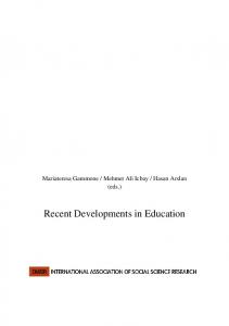
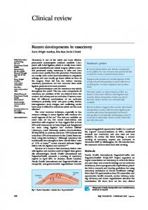
Multiple hypothesis testing - recent developments and future challenges [PDF]

Recent Advances and Developments in Neural ... - Bentham Openhttps://www.researchgate.net/.../Recent-Advances-and-Developments-in-Neural-Repair...

Recent Developments in LS-DYNA®

Recent Developments in Family Psychoeducation

Recent Developments in Tolerancing Techniques

Recent developments in the asymmetric

Recent Developments in Intergenerational Mobility

Recent developments in magneto-hydrodynamic

Recent Developments in Cfengine - CiteSeerX

Recent developments in photocatalytic water