The Astronomical Journal, 154:145 (15pp), 2017 October
https://doi.org/10.3847/1538-3881/aa88b8
© 2017. The American Astronomical Society. All rights reserved.
Precise and Fast Computation of the Gravitational Field of a General Finite Body and Its Application to the Gravitational Study of Asteroid Eros Toshio Fukushima National Astronomical Observatory/SOKENDAI, Ohsawa, Mitaka, Tokyo 181-8588, Japan;
[email protected] Received 2017 July 16; revised 2017 August 24; accepted 2017 August 26; published 2017 September 15
Abstract In order to obtain the gravitational field of a general finite body inside its Brillouin sphere, we developed a new method to compute the field accurately. First, the body is assumed to consist of some layers in a certain spherical polar coordinate system and the volume mass density of each layer is expanded as a Maclaurin series of the radial coordinate. Second, the line integral with respect to the radial coordinate is analytically evaluated in a closed form. Third, the resulting surface integrals are numerically integrated by the split quadrature method using the double exponential rule. Finally, the associated gravitational acceleration vector is obtained by numerically differentiating the numerically integrated potential. Numerical experiments confirmed that the new method is capable of computing the gravitational field independently of the location of the evaluation point, namely whether inside, on the surface of, or outside the body. It can also provide sufficiently precise field values, say of 14–15 digits for the potential and of 9–10 digits for the acceleration. Furthermore, its computational efficiency is better than that of the polyhedron approximation. This is because the computational error of the new method decreases much faster than that of the polyhedron models when the number of required transcendental function calls increases. As an application, we obtained the gravitational field of 433 Eros from its shape model expressed as the 24×24 spherical harmonic expansion by assuming homogeneity of the object. Key words: celestial mechanics – gravitation – minor planets, asteroids: individual (433 Eros)
types (Laplace 1799):
1. Introduction Spurred by the achievement of the asteroid explorer HAYABUSA (Fujiwara et al. 2006), the JAXA launched its successor, HAYABUSA2, on 2014 December 3. It is scheduled to land on the asteroid 162173 Ryugu in 2018 June–July (Tsuda et al. 2013). In order to assist the descending orbit design of the spacecraft and its probe MASCOT (Matsuoka & Russell 2017), we started an investigation to accurately compute the gravitational field of Ryugu when its detailed information becomes available (Müller et al. 2016). Of course, the computation of the gravitational field of a general object has been a classic problem in astronomy and geodesy since the days of Newton (Heiskanen & Moritz 1967; Binney & Tremaine 2008). However, analytical solutions are known only for limited types of objects (Chapman 1979; Heck & Seitz 2007; Wild-Pfeiffer 2008): (i) a general spherically symmetric object, as shown by Newton himself (Chandrasekhar 1995), and a homoeoid as its ellipsoidal generalization (Chandrasekhar 1969), (ii) a homogeneous body with simple shapes such as an infinitely fine straight line segment (Kellogg 1929; Chapter 3, Section 3, Excers. 1), an infinitely thin rectangle (Fukushima 2016b), a rectangular parallelepiped (MacMillan 1930), a polyhedron as its generalization (Paul 1974), an infinitely fine circular ring (Kellogg 1929; Chapter 3, Section 4), an infinitely thin circular disk (Fukushima 2010), and a triaxial ellipsoid (Byrd & Friedman 1971; Introduction, Example III), and (iii) an inhomogeneous case, such as a polyhedron with a density distribution described by a linear function and low-degree polynomials (Garcia-Abdeslem 1992). Consequently, for a general volume mass density distribution of the object, r (x), a possible approach to obtain its gravitational field is the numerical quadrature of the following
V (X ) º G a (X ) º
r (x )
ò ∣x - X ∣ d 3x,
¶V =G ¶X
ò
r (x)(x - X ) 3 d x, ∣ x - X ∣3
(1 ) (2 )
where G is Newton’s gravitational constant, X is the point of evaluation, x is the point of an internal mass element, V (X ) is the negative gravitational potential, and a (X ) is the gravitational acceleration vector. Nevertheless, the kernel functions of these convolution integrals contain algebraic singularities of the orders of 1 and 2. As a result, their proper integration has been difficult (Klees & Lehmann 1998). If the object is finite, on the other hand, V (X ) satisfies the Laplace equation outside the object. As a result, V (X ) can be expanded as an infinite series of basis functions satisfying the Laplace equation in some selected coordinate systems (Hobson 1931). In this case, an issue to be resolved is the precise and fast computation of the basis functions termed the harmonics for arbitrary combination of their indices, parameters, and/or arguments. In the past decades, this problem has been positively solved: the spherical harmonics (Fukushima 2012a, 2012b, 2012c, 2014c), the oblate spheroidal harmonics (Fukushima 2013), the prolate spheroidal harmonics (Fukushima 2014a), the triaxially ellipsoidal harmonics (Garmier & Barriot 2001, 2002), and the axisymmetric toroidal harmonics (Fukushima 2016c). For instance, high-degree and high-order spheroidal harmonic expansions are successfully determined for the asteroids Bennu and Castalia (Sebera et al. 2016). However, we warn the readers that even outside the object, the harmonic expansions do not always converge uniformly (Moritz 1980). The domain of the convergence is called the 1
The Astronomical Journal, 154:145 (15pp), 2017 October
Fukushima
Figure 2. Effective order of the gravitational potential computation. Shown are p º [log10 (dV0 dV )] (log10 Nfunc ), the effective order of computing the gravitational potential of the asteroid Eros at its coordinate center. The polyhedron models (D’Urso 2014a), marked by open circles, and the new method, indicated by filled circles, are compared. Here dV is the relative error measured as the difference with the reference solution obtained by the quadruple precision integration with a tiny value of the input relative error tolerance, Nfunc is the number of transcendental function evaluations such as the logarithm, trigonometric, and inverse trigonometric functions, and dV0 = 0.015 is a numerical constant so that the results of the polyhedron model reproduce the theoretical value of the effective order, p=1. The effective orders of the new method are not constant but increase exponentially with respect to Nfunc . The broken line shows its model curve expressed as pmodel = [exp (0.47 log10 Nfunc ) - 2.0] (log10 Nfunc ).
Figure 1. Sketch of the Brillouin sphere. Shown is a meridional cross-section of a finite body expressed by a solid curve, RT (f, l ), and its Brillouin sphere, namely the minimum concentric sphere including the body, indicated by a broken curve. Filled squares denote the origin, O, a point inside the body, P1, a point on the surface of the body, P2, a point outside the body but inside its Brillouin sphere, P3, and a point outside the Brillouin sphere, P4.
2015b; Wang et al. 2014, 2016; Jiang & Baoyin 2016). This popularity is supported by a number of theoretical and computational developments in polyhedron models (Nagy 1966; Barnett 1976; Okabe 1979; Waldvogel 1979; Pohanka 1988, 1998; Werner 1994, 1997; Holstein & Ketteridge 1996; Petrovic 1996; Holstein et al. 1999; Nagy et al. 2000; Scheeres et al. 2000; Smith 2000; Garcia-Abdeslem & Martin-Atienza 2001; Singh & Guptasarma 2001; Smith et al. 2001; Tsoulis & Petrovic 2001; Holstein 2002, 2003; Korycansky 2004; GarciaAbdeslem 2005; Werner & Scheeres 2005; Fahnestock & Scheeres 2006; Hamayun et al. 2009; Tsoulis et al. 2009; Tsoulis 2012; D’Urso 2013, 2014b; Takahashi et al. 2013; Chanut et al. 2015a; D’Urso & Trotta 2015; Zhao et al. 2016). Nevertheless, the polyhedron model is only an approximation. Indeed, its approximation error is non-negligible even if the polyhedron field itself is precisely computed (Conway 2015). For example, an analysis of the computed values of the gravitational potential of Eros at its coordinate center for the four polyhedron models with a different number of faces, Nface = 1708, 7790, 10,152, and 22,540 (D’Urso 2014a), revealed that the computational error is inversely proportional to Nface . Since the computational labor is in proportion to Nface , the polyhedron model is an approximation method on the order of one as
Brillouin manifold (Jekeli 2007). We illustrate in Figure 1 its spherical example, the Brillouin sphere. When the shape of the object is as complicated as that of asteroid Itokawa (Müller et al. 2014), the domain inside the Brillouin manifold but outside the object is not negligibly small. Thus, attempts to utilize the harmonic expansions only in evaluating the external gravitational field of such objects are problematic, especially in designing the descending orbit of a space probe such as HAYABUSA2/MASCOT (Watanabe et al. 2017). Some trials exist, however, to represent the solution in the outside of the object as a combination of not the external but the internal harmonic expansions around different coordinate centers (Takahashi et al. 2013). The internal/external series expansions using the spherical Bessel functions has also recently been proposed (Takahashi & Scheeres 2014). Among these, the conditional switch of multiple internal harmonic expansions with different coordinate centers was recommended (Takahashi & Scheeres 2014). Nonetheless, its realization is cumbersome if the entire exterior domain of irregular shaped objects is to be covered, such as is the case of the asteroid Eros (Zuber et al. 2000). This is the reason why polyhedron models have been widely adopted in computing the gravitational field of asteroids, comets, and small satellites (Scheeres 1994; Werner & Scheeres 1997; Miller et al. 2002; Thomas et al. 2002; Hikida & Wieczorek 2007; Konopliv et al. 2014; Park et al. 2014; Lhotka et al. 2016; Zhao et al. 2016; Aljbaae et al. 2017). In fact, they are frequently used in the dynamical study of orbits around such objects (Scheeres et al. 1996, 1998, 2000; Rosshi et al. 1999; Hu & Scheeres 2004, 2008; Yu & Baoyin 2012a, 2012b, 2013, 2015; Li et al. 2013, 2017a; Chanut et al. 2014,
dV = dV0 (Nfunc)-1,
(3 )
where dV is the relative error measured as the difference with the reference solution, Nfunc is the number of transcendental function evaluations required in the potential computation such as the logarithm and inverse trigonometric functions, and dV0 = 0.015 is a numerical constant. Figure 2 illustrates the 2
The Astronomical Journal, 154:145 (15pp), 2017 October
Fukushima
effective order defined as pº
log10 (dV0 dV ) . log10 Nfunc
polyhedron model in evaluating the gravitational potential of Eros. Clearly, the new method has a higher cost performance since its effective order is typically higher than that of the polyhedron model, especially when high precision is required. Below, we explain the new method in Section 2 and present its numerical experiments in Section 3. We also prepared the appendices containing the derivation of the formulas used in the new method, the description of the coefficient functions in the transformed integrand, a rewriting of the integrand to avoid the cancellation in its computation when the object consists of thin layers, a pair of Fortran subroutines to execute the DE quadrature in the double and quadruple precision environment, respectively, the results of some numerical experiments to confirm their good cost performance, and a Fortran function to compute a special logarithm function that is the key component of the integrand evaluated in the new method.
(4 )
In the figure, the open circles show the results of the polyhedron models. The constant value of p indicates that the relative error decreases in proportion to (Nfunc )-p , where Nfunc is obtained from Nface as Nfunc = 3.5Nface in the computational procedure of the polyhedron models (D’Urso 2014a). In any case, the observed order of the polyhedron models is too low to obtain precise gravitational fields efficiently. This is the reason why, in geodesy, the polyhedron models are not intensively investigated, but the high-order numerical quadrature of the tesseroid1 models is, though no analytical solution is known for the gravitational field of a tesseroid and its spheroidal extension, and therefore the computational cost of its numerical integration is high (Huang et al. 2001; Novak & Grafarend 2005; Asgharzadeh et al. 2007; Han & Shen 2010; Tsoulis 2012; Tsoulis et al. 2012; Grombein et al. 2013; Hirt & Kuhn 2014; Du et al. 2015; Roussel et al. 2015; Shen & Deng 2016; Wu 2016). Recently, we have completely resolved the problem of the algebraic singularities in V (X ) and a (X ) (Fukushima 2016e). The key to success is the regularization of the Newton kernels, 1 ∣x - X∣ and/or 1 ∣x - X∣2 , by the integral variable transformation using the spherical polar coordinates centered at the evaluation point. The rewritten forms of V (X ) and a (X ) can be properly integrated for any form of r (x) by the standard numerical quadrature methods (Press et al. 2007; Chapter 4). Having said that, we must confess that the computational burden to integrate them is huge (Fukushima 2016e; Figures 15 and 16). This is because the regularized integrals remain threedimensional. In the case of solar system objects, r (x) is piecewise constant or well approximated by a low-degree polynomial in the radial direction. This fact enables us to reduce the dimension of the potential integration from three to two, as we show below. After the reduction, nevertheless, the integrand of the two-dimensional integral of the gravitational potential becomes logarithmically singular if the evaluation point is on the surface of or inside the object. Of course, the singularity is weak and therefore integrable in principle. However, their numerical integration has been difficult (Klees 1996). We have conquered this difficulty (Fukushima 2016a, 2016d) by the combination of the split quadrature method (Fukushima 2014b) using the double exponential (DE) rule (Takahashi & Mori 1973, 1974) for the potential integration and the numerical differentiation of the numerically integrated potential by Ridders’ method (Ridders 1982) for the acceleration computation. Later, we realized that Ridders’ method can be replaced by its simpler substitute: the central or single-sided difference formulas with an appropriate choice of the trial argument difference (Fukushima 2017). This replacement is in order to decrease the computational cost of the device. Using the improved formulation, we succeeded to construct a precise and fast method of the gravitational field computation of a general finite body. We again refer to Figure 2. It compares the cost performance of the new method with that of the
2. Method 2.1. Surface Integral Expression of the Gravitational Potential Let us consider the gravitational potential of a general finitebody-like solar system object. It is mathematically described as a volume integral in Equation (1). Without losing generality, we assume that the body is composed of multiple layers and all the layers are well defined in a certain spherical polar coordinate system associated with the object. If this assumption is not satisfied in a single spherical polar coordinate system, such as in the case of comet 67P Churyumov–Gerasimenko (Jorda et al. 2016), one may separate the finite body into some pieces so that the radial uniqueness condition is satisfied in each piece after taking different spherical polar coordinate systems with appropriate shift of the coordinate centers. We denote by RT (f, l ) and RB (f, l ) the radii of the top and the bottom surfaces of the layer, respectively. They are uniquely defined as functions of the latitude f and the longitude λ. We also write the volume mass density of the layer as r (r, f, l ), where r is the radius vector. Hereafter, we focus on the gravitational field of a single layer. Within the layer, we assume that r (r, f, l ) is properly expanded as a low-degree polynomial of r as r (r , f , l ) =
⎛ r ⎞n r f , l ( ) ⎜ ⎟ , å n ⎝ R0 ⎠ n=0 N
(5 )
where R0 is a certain reference value of the radius and N is a certain integer, say, in the range of 0–5. In fact, the density profile of the Earth is approximated by piecewise linear or cubic polynomials (Dziewonski & Anderson 1981; Kennett 1998; Ganguly et al. 2009). The density profile of the tropospheric air mass can also be represented by a quintic polynomial (Karcol 2011). The separation of r n from the full expression of the density profile, r (r, f, l ), is a central trick of the new method. Indeed, as we show below, the kernel function can be analytically integrable even after the inclusion of r n. The gravitational potential of the layer at an arbitrary point is written as a similar finite series as V ( R , F , L) =
N
å Vn (R, F , L) ,
(6 )
n=0 1
A tesseroid is a finite volume enclosed by two meridians, two parallels, and two spherical surfaces (Anderson 1976). It is sometimes called a spherical prism.
where (R, F, L) are the spherical polar coordinates of the evaluation point. Each term of the potential is expressed as a 3
The Astronomical Journal, 154:145 (15pp), 2017 October
Fukushima
⎛ 5 ⎞ (18) C1 º (a - B) ⎜a2 - 5aB + B 2⎟ , ⎝ 2 ⎠ ⎛ 35 5 ⎞ ⎛3 5 ⎞ 1 D1 º ⎜3a2 aB + B 2⎟ + ⎜ a - B⎟ z + z 2, ⎝ 6 2 ⎠ ⎝2 6 ⎠ 3 (19)
volume integral in the spherical polar coordinate system as G R0
Vn (R , F , L) º
´
p 2
⎡
2p
ò-p 2 ⎢⎣ò0
⎛ rn (f , l) ⎜ ⎝
R T (f, l )
òR (f,l) B
⎞ ⎤ ⎛r r2 ⎜ ⎟ dr ⎟ dl⎥ cos f df. S (r , f , l) ⎝ R 0 ⎠ ⎠ ⎥⎦ ⎞n
(7 )
C2 º a4 - 10a 3B +
Here S (r, f, l ) is a square root representing the normalized distance between the internal and evaluation points as S (r , f , l ) º
A (f , l) + [B (f , l) + z ]2 ,
where A (f, l ) and B (f, l ) are a pair of auxiliary functions defined as (9 )
⎡ ⎛x ⎞ ⎛ h ⎞⎤ B (f , l) º 2a ⎢sin2 ⎜ ⎟ + cos f cos F sin2 ⎜ ⎟ ⎥ , ⎝ 2 ⎠⎦ ⎝2 ⎠ ⎣
(10)
⎛ 77 63 3 63 4⎞⎟ C3 º (a - B) ⎜a4 - 14a 3B + a2B 2 aB + B , ⎝ 2 2 8 ⎠ (22)
and α, ξ, η, and ζ are non-dimensional quantities defined as aº
R r-R , x º f - F, h º l - L, z º . R0 R0
⎛ 85 3 1001 2 2 273 3 63 4⎞⎟ D 3 º ⎜5a4 aB+ aB aB + B ⎝ 3 20 8 8 ⎠ ⎛ 145 2 399 2 21 3⎞⎟ + ⎜5 a 3 aB+ aB B z ⎝ 12 40 8 ⎠ ⎛ 10 69 21 2⎞⎟ 2 + ⎜ a2 aB + B z ⎝ 3 20 20 ⎠ ⎛5 9 2⎟⎞ 3 1 +⎜ aB z + z 4, ⎝4 20 ⎠ 5 (23)
(11)
The innermost line integral of Vn (R, F, L), namely that with respect to r, can be analytically evaluated in a closed form as explained in Appendix A. As a result, Vn (R, F, L) is rewritten as a surface integral as Vn (R , F , L) = GR 02
p 2
⎛
ò-p 2 ⎜⎝ò0
2p
⎞ rn (f , l) Kn (f , l) dl⎟ cos fd ⎠ (12)
where Kn (f, l ) is the kernel function of degree n defined as a difference of integrals as Kn (f , l) º In (RT (f , l) , f , l) - In (RB (f , l) , f , l) ,
where we dropped the argument dependence for simplicity. Refer to Appendix A for a recursive algorithm to obtain the coefficient functions of arbitrarily high degrees. The correctness of the analytical expression of In (r, f, l ), Equation (14), is easily confirmed by its direct differentiation with respect to r. Originally, the functions S (r, f, l ), A (f, l ), and B (f, l ) are expressed as
(13)
while In (r, f, l ) is an indefinite line integral defined and analytically expressed as In (r , f , l) º
(r ¢)n + 2 dr ¢ = Cn (f , l) L (r , f , l) S (r ¢ , f , l ) + Dn (r , f , l) S (r , f , l). (14) 1
R 0n + 3
ò
r
S (r , f , l ) =
L (r , f , l ) ⎧ ln [S (r , f , l) + B (f , l) + z ] , (B (f , l) + z 0) , ⎪ º⎨ ln [A (f , l) {S (r , f , l) ⎪ - B (f , l) - z}] , (B (f , l ) + z < 0 ) , ⎩
(24) (25) (26)
where ψ is the spherical angle between the direction vectors toward the internal and the evaluation points from the coordinate center, such that cos y = sin f sin F + cos f cos F cos (l - L).
(15)
(27)
Nevertheless, the computation of ψ from this conventional definition suffers from a cancellation problem when f » F and l » L, and therefore y » 0. This is the reason why we use the rewritten expressions of A (f, l ) and B (f, l ), Equations (9) and (10), which are robust against the smallness of x = f - F and h = l - L. Refer to Appendix A for a more detailed explanation. The analytical expression of In (r, f, l ), Equation (14), is not found in the literature. Although the lowest degree
and Cn (f, l ) and Dn (r, f, l ) are the coefficient functions of degree n defined as polynomials of B (f, l ), α, and ζ. The first four pairs are explicitly displayed here as 3 2 B , 2 ⎛ 3 ⎞ 1 D 0 º ⎜2a - B⎟ + z , ⎝ ⎠ 2 2
R 2 - 2rR cos y + r 2 , R0
A (f , l) = a2 sin2 y, y B (f , l) = 2a sin2 , 2
Here L (r, f, l ) is a logarithmic function conditionally defined as
C0 º a2 - 3aB +
(20)
⎛ 43 2 175 2 35 3⎞⎟ D 2 º ⎜4a 3 aB+ aB B ⎝ 3 12 8 ⎠ ⎛4 ⎛ 49 35 2 ⎟⎞ 7 ⎞⎟ 2 1 + ⎜3a 2 aB + B z+⎜ aB z + z 3, ⎝ ⎝3 12 24 ⎠ 12 ⎠ 4 (21)
(8 )
A (f , l) º B (f , l)[2a - B (f , l)] ,
45 2 2 35 3 35 4 aB aB + B , 2 2 8
(16) (17)
4
The Astronomical Journal, 154:145 (15pp), 2017 October
Fukushima
angular coincidence, namely when x = h = 0 . Therefore, we first change the integration variables from f and λ to ξ and η, respectively. Next, we split the integration interval of ξ into positive and negative parts. In general, one must also split the integration interval of η similarly. However, we only have to shift the transformed integration interval as [0, 2p ) in terms of not λ, but η. This is because the integrand is of 2p periodicity with respect to λ. The final form of the split quadrature becomes
expression, I0 (r, f, l ), is mathematically equivalent with the existing form (Heck & Seitz 2007; Equation(20)), the rewritten expression here is numerically more stable in the sense that no cancellation occurs when ξ and η are small, then A (f, l ) and B (f, l ) are also small, thus S (r, f, l ) » ∣z ∣, and therefore L (r, f, l ) » ln (z + ∣z ∣) becomes large if z < 0 . Note that if the layer is thin, the above expression of the kernel functions in a differenced form, Equation (13), suffers from another kind of information loss. Refer to Appendix B for its cancellation-free rewriting. The robustness of the rewritten kernel functions is the key factor to ensure an accurate integration of the gravitational potential, as we show below.
Vn (R , F , L) =
0
ò-p 2-F Pn (x ) dx + ò0
p 2 -F
Pn (x ) dx ,
(28)
where the new integrand Pn (x ) is a definite line integral defined as 2.2. Split Quadrature Method Using the Double Exponential Rule
Pn (x ) º
Now, the problem is reduced to the evaluation of a weakly singular two-dimensional integral. Since the integral cannot be analytically evaluated in a closed form, we evaluate it by a method of numerical quadrature. When the evaluation point is inside or on the surface of the layer, the kernel functions, Kn (f, l ), contain a logarithmically blowing-up singularity at the point of angular coincidence, namely when x = h = 0 . This is because, in this case, the argument of the logarithm in L (r, f, l ) reduces to the form of z + ∣z ∣, which can completely vanish if z 0 . In addition, even if the evaluation point is outside the layer, such that z > 0 , the main functions, L (r, f, l ) and S (r, f, l ), have a sharp peak or a steep kink at the point of angular coincidence when ∣z ∣ is sufficiently small. In such cases, the behavior of the integrand is difficult approximate as a low-degree polynomial, which is the commonly assumed condition on which most of the ordinary quadrature rules are based. As a result, practical difficulties appear in the numerical integration by the standard numerical integrators like the Gauss–Legendre quadrature or the Romberg rule (Press et al. 2007; Chapter 4). In order to circumvent this difficulty, we adopt the DE rule (Takahashi & Mori 1973, 1974) as a method of numerical integration. In short, the DE rule is the Romberg rule applied to the integrand transformed by the so-called TANH–SINH transformation and other integral variable transformations of DE nature (Press et al. 2007; Section 4.5). It is known as one of the best quadrature rules (Bailey et al. 2005). This is because the integration error typically decreases exponentially with respect to the number of integrand evaluations. Moreover, the DE rule is easy to use since its algorithm is adaptive. In fact, one only has to specify δ, the input relative error tolerance. Then, the algorithm automatically takes care of test integrations in the Romberg rule so as to minimize the number of integrand evaluations while satisfying the error requirement. Experimentally, we learn that the algorithm is so reliable in the sense that the achieved relative errors are usually smaller than the input requirement if the length of the integration interval after the transformation is appropriately chosen. For the readers’ convenience, we added Appendix C, where we describe dqde, a Fortran subroutine of the DE rule in the double-precision environment with an optimal setting of the integration interval. The DE rule is known to be able to integrate weakly singular and/or nearly singular integrals properly if the singularities and/or the point of peaks are located at the endpoints of the integration interval (Mori 1985). In the present case, the singularities and/or the sharp peaks are located at the point of
ò0
2p
Q n (x , h ) d h ,
(29)
while Qn (x , h ) is an abbreviation expressed as Qn (x , h ) º GR 02 rn (F + x , L + h ) Kn (F + x , L + h ). (30)
Of course, if the object is homogeneous, then we can set N = 0 and simplify the integrand Q0 as Q0 (x , h ) = GR02 r00 K0 (F + x , L + h ), where r00 is the constant density value of the object. We evaluate all the line integrals in Equations (28) and (29) by the DE rule. 2.3. Numerical Differentiation Let us move on to the computation of the gravitational force. In this case, the situation is significantly different. Even after the radial integration is analytically conducted, the numerical integration of its surface integral form suffers from the algebraic singularities (Klees & Lehmann 1998). Therefore, we adopt another approach: the numerical partial differentiation of the numerically integrated potential (Fukushima 2016a, 2016d, 2017). Namely, assuming the availability of V (X ) for arbitrary values of X , we obtain a (X ), and other quantities defined as the partial derivatives in general, by numerically evaluating their definitions as partial derivatives of V (X ). As the method of numerical differentiation, we previously used Ridders’ method (Ridders 1982). Of course, this is a sure method. Nevertheless, it is also true that its computational cost is significantly higher, say a few tens of times more, than that of the potential. Thus, in order to reduce the computational labor while maintaining as high an accuracy as possible, we replace it with a conditional switch between the central difference formula and the single-sided difference formulas (Fukushima 2017). More specifically speaking, as long as the following test displacement of the evaluation point does not cross the surface of the layer, we approximate the gravitational acceleration components in the spherical polar coordinate system by the central difference formula as aR (R , F , L) » [V (R + DR , F , L) - V (R - DR , F , L)] (2DR) ,
(31)
a F (R , F , L) » [V (R , F + DF , L) - V (R , F - DF , L)] (2RDF) ,
(32)
aL(R , F , L) » [V (R , F , L + DL) - V (R , F , L - DL)] [2 (R cos F) DL] , (33)
5
The Astronomical Journal, 154:145 (15pp), 2017 October
Fukushima
by setting the test displacements in the spherical polar coordinates as DR R = DF = DL = d2,
components if the evaluation point is far from the surface and the six-digit accuracy if near the surface. The computational cost for each component of the acceleration vector is twice higher than that of the gravitational potential when the central difference formula is employed. Thus, the total CPU time to obtain the full acceleration vector becomes six times longer. On the other hand, when the singlesided difference formula is used, the extra computational cost per component is the same as that of the potential. Since the base potential value can be shared, the total computational labor is only four times greater.
(34)
where we set the relative displacement as d2 =
3
d.
(35)
This expression of the test displacement is obtained by equating the approximation error of the central difference formula with the input relative error of the potential integration (Press et al. 2007; Section 5.7) after approximating the behavior of the potential and its third-order partial derivatives as those of a masspoint. On the other hand, if any of the above test displacements crosses the surface of the layer, we compute the gravitational acceleration vector by appropriately chosen single-sided difference formulas such as
3. Numerical Experiments 3.1. Homogeneous Spherical Layer Below, we show the computational performance of the new method. Let us begin with the case where the analytical solution is known: a homogeneous spherical layer. We denote the reference radius and the top and bottom surface radii of the layer by R0, RT , and RB, respectively. Then, the gravitational potential of the layer at a given radius R is expressed as
aR (R , F , L) » [V (R + DR , F , L) - V (R , F , L)] (DR) , (36) a F (R , F , L) » [V (R , F + DF , L) - V (R , F , L)] (RDF) , (37) aL(R , F , L) » [V (R , F , L + DL) - V (R , F , L)] [(R cos F) DL] ,
V (R ) ⎧ 2pGr (RT + RB ) H , (0 R < RB) , ⎪ 2 3 2 º ⎨(2pGr 3)(3RT - R - 2RB R) , (RB R < RT) , ⎪ (RT R) , ⎩GM R ,
(38)
or
(44)
aR (R , F , L) » [V (R , F , L) - V (R - DR , F , L)] (DR) , (39)
where ρ is the constant density of the layer, H º RT - RB is the thickness of the layer, and M is the mass of the layer, expressed as
a F (R , F , L) » [V (R , F , L) - V (R , F - DF , L)] (RDF) , (40)
M º (4p 3) r (RT2 + RT RB + RB2 ) H .
aL(R , F , L) » [V (R , F , L) - V (R , F , L - DL)] [(R cos F) DL]. (41)
The radial component of the gravitational force is expressed as dV (R) dR ⎧ 0, (0 R < RB) , ⎪ 3 2 = ⎨(4pGr 3)( - R + RB R ) , (RB R < RT) , ⎪ (RT R). ⎩- GM R 2 ,
a (R ) º
This time, we set the test displacements in the spherical polar coordinates as DR R = DF = DL = d1,
(42)
where a new relative displacement is chosen as d1 =
d.
(45)
(43)
(46)
As a test case, we set R0 = 6380 km , RT = R0 + 10 km , and RB = R0 - 40 km so as to model a spherical crust of the Earth. Then, we measured the relative errors of the gravitational potential integrated by the new method by comparing with the exact solution as
It is determined by equating the approximation error of the single-sided difference formulas with the input relative error of the potential integration (Press et al. 2007; Section 5.7) after approximating the behavior of the potential and its secondorder partial derivatives as those of a masspoint. Of course, the input relative error tolerance of the potential integration, δ, is different from the achieved accuracy of the potential integrated. However, as we show below, we confirm that δ is a reliable indicator of the actual integration error. Therefore, we used the former as an appropriate estimate of the latter. The expected relative accuracy of the thus approximated gravitational acceleration vector is d 22 = 3 d 2 for the central difference formulas and d1 = d for the single-sided difference formulas, respectively. For example, if we set d = 10-12 , then d2 = 10-4 and d1 = 10-6 , and we may therefore anticipate the eight-digit accuracy of the gravitational acceleration
dV º (Vintegrated - Vexact ) Vexact.
(47)
Figure 3 illustrates the measured errors as functions of R for various values of δ, the input relative error tolerance, in a logarithmic manner. The obtained errors are almost constant with respect to R, namely they are independent of the location of the evaluation point. The relative errors of the integrated potential is roughly the same as δ if d > 10-10 . Otherwise, the errors increase by about a factor 30. Let us move to the error of the computed acceleration vector. This time, the relative errors are not well defined since the exact 6
The Astronomical Journal, 154:145 (15pp), 2017 October
Fukushima
Figure 4. Normalized error of the gravitational acceleration of the spherical layer. Same as Figure 3 but for the normalized errors of a º ∣a∣, the magnitude of the gravitational acceleration vector, defined as da º (a integrated - aexact ) a max . Here a max is the maximum value of the acceleration, namely that at R = RT .
Figure 3. Relative error of the gravitational potential of the spherical layer. Plotted are the base-10 logarithm of the magnitude of the relative errors of the gravitational potential, dV º Vintegrated Vexact - 1. Shown are the results for some values of δ, the input relative error tolerance for the DE quadrature rule as d = 10-6 , 10−8, 10−10, 10−12, 10−14, and 10−16 in the double-precision environment.
value vanishes when R < RB. Instead, we introduce the normalized error of acceleration defined as da º (a integrated - a exact ) a max ,
(48)
where a max º a (RT ) is the maximum value of a(R). Figure 4 depicts the normalized errors of the gravitational acceleration computed by the new method as functions of R. This time, they are mostly unchanged if outside the layer. In fact, the measured errors are roughly equal to 3 d 2 as we expected. Inside the layer, however, the errors increase roughly by a factor of 10–30. Also, the errors become large near the surface, say 6 ´ 10-5 when d = 10-12 . If we add the contribution of the main part of the Earth, namely that of its mantle and core, the relative magnitude of the computational errors of the crustal component become much smaller, say, by a factor of 10−3–10−4. Therefore, we think that the new method can be sufficiently accurate in the computation of the gravitational field. This is the case if the considered body is nearly spherical in the sense that the contribution of the nonspherical part is relatively small such as the cases of Ceres, Vesta, Deimos, Phobos, and especially the asteroid Ryugu, the target object of the HAYABUSA2mission (Müller et al. 2016). Finally, we measure the computational labor of the new method. Figure 5 depicts Nfunc , the number of transcendental function evaluations required in computing the gravitational potential of the spherical layer by the new method. The figure illustrates the R-dependence of Nfunc . We omit the similar graphs showing the Φ- and Λ-dependences, respectively, since the results are practically the same as those depicted in Figure 5. At this scale, the computational cost seems to be independent on the location of the evaluation point. This situation is the same as in the polyhedron model. However, as will be seen later, the computational cost in actual cases reduces when the distance from the object increases significantly.
Figure 5. Integration cost of the gravitational potential of the spherical layer. Same as Figure 3 but plotted is the base-10 logarithm of Nfunc , which is directly in proportion to the total CPU time. Obviously, the computational labor is almost independent of the location of the evaluation point. Sometimes, the total number is changed by a factor of 1.5, which corresponds to a constant step in the graph amounting to log10 1.5 » 0.176 . This incremental factor of 1.5 corresponds to the doubling of the number of evaluation for one part of the split integral evaluation, which is caused because the DE rule is based on the Romberg quadrature method, which automatically increases the number of integrand evaluation points in its test integrations by the mid-point rule.
3.2. Asteroid Eros As a more realistic example, let us investigate the gravitational field of 433 Eros. This is one of the most difficult cases of the gravitational field computation because the shape of the asteroid is significantly irregular. As its surface function, RT (f, l ), we used the 24×24 spherical harmonic expansion (Miller et al. 2002). Its bird’s eye view as well as the associated contour map are shown in Figure 6. By setting RB (f, l ) = 0 for simplicity and assuming the homogeneity of the asteroid, we integrated the gravitational potential, V (R, F, L), by setting d = 10-12 , and computed the acceleration vector, a (R, F, L), by setting d2 = 10-4 far from the surface and d1 = 10-6 near the surface. 7
The Astronomical Journal, 154:145 (15pp), 2017 October
Fukushima
Figure 6. Surface function of Eros. Shown are a bird’s eye view and the associated contour map of the surface function of the asteroid Eros. Displayed is its shape modeled by a 24×24 spherical harmonic expansion (Miller et al. 2002) after normalization with R0 = 5.99276 km , the reference radius defined as that at the north pole, f = +90. Two high mountains are actually the two edges of the elongated shape of the Eros. The maximum and minimum normalized radii are 2.9439 and 0.4902, achieved at (f, l ) = (-410¢ , 18655¢) and (+1302¢ , 27327¢), respectively.
Figure 8. Gravitational acceleration of Eros on a spherical surface, R = 2 R0 . Same as Figure 7 but for the magnitude of the gravitational acceleration vector, a (R, F, L) º ∣a (R, F, L)∣. This time, the normalization constant is defined as a 0 º (4p 3) GrR0 , namely the surface acceleration of a sphere of the radius R0 with the same density. The acceleration magnitude becomes locally maximum at two oval-shaped curves. They roughly represent the cross-sections of the surface of the asteroid cut by the sphere of radius, R = 2 R0 .
Figure 7. Gravitational potential of Eros on a spherical surface, R = 2 R0 . Same as Figure 6 but for the gravitational potential of Eros on the spherical surface of a constant radius. Displayed is the result when R = 2 R0 . The corresponding spherical surface is inside the Brillouin sphere but outside the bottom of the surface of Eros. The potential values are obtained by the new method with a sufficiently small relative error tolerance, d = 10-12 . The normalization constant of the potential is V0 º (4p 3) GrR02 , the surface potential value of a sphere of the radius R0 with the same density. The curved surface of the potential mostly follow the bipolar feature of the surface function. However, the variation of the potential value is much smoother than that of the surface radius. This is due to the global nature of the gravitational field. A careful examination will reveal the nonanalyticity of the obtained curved surface of the potential value at the loci where R = RT (f, l ). Nevertheless, it is hardly visible at this scale.
Figure 9. Equatorial cross-section of the gravitational potential of Eros. Depicted is the contour map of V (R, 0, L), the gravitational potential of Eros on its equatorial cross-section, namely when F = 0 . The X and Y coordinates are defined as X º R cosL and Y º R sinL .
had experienced with that of the spiral galaxy M74 (Fukushima 2016b). On the other hand, those of the acceleration magnitude have a sharp kink on two oval-shaped loci. They roughly correspond to the cross-section of the surface of Eros cut by the sphere of constant radius, R = 2 R0 . This is natural because the density is discontinuous across the loci: finite inside the loci and zero outside them. In order to show the nonanalyticity of the gravitational field more clearly, we prepared Figures 9 and 10, displaying the contour map of the gravitational potential and the magnitude of the gravitational acceleration evaluated on the equator, namely when F = 0, respectively. The contours of the potential value become dense near the surface of the object. This implicitly shows the nonanalyticity there. The situation is similar to that of the potential map of some finite axisymmetric bodies (Fukushima 2016d, AppendicesA and C). Also, the contours of the acceleration magnitude exhibit a sharp boundary, which exactly coincides with the surface of the object. This is the
Figures 7 and 8 depict a bird’s eye view and the associated contour map of the integrated potential and the magnitude of the computed acceleration vector at a constant radius, respectively. They are drawn as two-dimensional maps with respect to the angular coordinates. The chosen radius, R = 2R0 , represents a case of the intermediate zone, namely inside the Brillouin sphere but above the bottom of the surface of the object. The displayed view/map of the potential are much smoother than those of the surface function (Figure 6). This is due to the averaging nature of the gravitational field computation as we 8
The Astronomical Journal, 154:145 (15pp), 2017 October
Fukushima
Figure 10. Equatorial cross-section of the magnitude of Eros’ gravitational acceleration. Same as Figure 9 but of a (R, 0, L), the magnitude of the gravitational acceleration on the equator. The obtained values of a have a clear kink on the surface of Eros. A careful comparison with Figure 9 reveals that the contours observed here are not the same as those of the gravitational potential. This is because the contribution of the longitudinal component of the acceleration cannot be retrievable from Figure 9 only.
Figure 11. Radial variation of the gravitational potential and the acceleration vector. Plotted are the radial variation of the gravitational potential and three components of the gravitational acceleration vector of the Eros along the direction of the lowest point where (F, L) = (+1302¢ , 27327¢). The vertical line is the location of the surface. Arrows indicate the peaks of gravitational acceleration components, which locate outside of the surface.
same feature we experienced with that of the spherical layer in the previous subsection. With an aim to clarify the nonanalytic feature of the gravitational field, we examined the radial variation of the gravitational field more closely. Refer to Figure 11, plotting the potential and the three acceleration components along the direction passing through the lowest point of the surface of Eros. Again, we confirm that the acceleration components are continuous but not differentiable at the surface. This is because the potential curves are not analytic there. We noticed that, even outside the object, all the acceleration components are not monotonically decreasing when R increases. The phenomenon is prominent near the surface, say, when 0.5 < R R0 < 0.7. Indeed, their peak values are achieved there. This interesting feature is caused by the gravitational attraction of the mountainous area surrounding the lowest point. On the other hand, Figure 12 illustrates the radial variation of the computational cost of the gravitational potential. When the distance from the asteroid is large, the potential value is almost inversely proportional to R, the radial coordinate. Therefore, for an efficient computation, one may increase the relative error tolerance so as to be in proportion to R. This policy decreases the computational cost as seen in Figure 12. This feature is different from the polyhedron model, which requries the same computational cost independently of the location of the evaluation point. Having said so, we must say that the spherical or spheroidal harmonic expansions are much more efficient if outside of the Brillouin sphere or spheroid. Let us focus on the gravitational feature on the surface, which is most difficult to obtain by the existing methods including the polyhedron models. Figure 13 illustrates the bird’s eye view and the associated contour map of the surface gravitational potential of the asteroid. By comparing it with Figure 6, we notice that the magnitude of the surface potential is inversely correlated with the shape function. Namely, it becomes small in the mountainous area and large in the basins and valleys.
Figure 12. Radial variation of computational cost of Eros’ potential. Shown is the radial variation of the computational cost of the gravitational potential of Eros along the direction of the lowest point, where (F, L) = (+1302¢ , 27327¢).
Figure 13. Surface gravitational potential of Eros. Same as in Figure 7 but on the surface of Eros. Namely, it displays VT (F, L) º V (RT (F, L), F, L).
9
The Astronomical Journal, 154:145 (15pp), 2017 October
Fukushima
Figure 15. Deflection of surface gravitational acceleration vector of Eros. Same as in Figure 13 but for the magnitude of the deflection angle of the gravitational acceleration vector, q º tan-1 ( aF2 + aL2 aR ), on the surface of Eros.
Figure 14. Magnitude of surface gravitational acceleration of Eros. Same as in Figure 13 but for the magnitude of the gravitational acceleration vector, aT (F, L) º ∣ a (RT (F, L), F, L)∣.
Next, we prepared Figure 14, showing the similar view and map of the magnitude of the surface gravitational acceleration vector of the asteroid. This time, the variation of the magnitude of the acceleration vector is significantly smaller than those of the potential. Also, the magnitude of the acceleration is smaller not only in the mountainous area but also in the basins and valleys. Third, we calculated the deflection angle of the surface acceleration vector, q º tan-1 ( a F2 + aL2 aR).
because the computational error of the new method decreases much faster than that of the polyhedron models when the computational labor is increased and partly because the integrand of the surface integral adopted in the new method calls only one transcendental function, a kind of special logarithm function, while the polyhedron models require one logarithm function for each edge and two arc tangent functions for each face to be computed. The author appreciates the referee’s valuable advice and comments, which improved the quality and readability of the present article.
(49)
Its bird’s eye view and the associated contour map are provided in Figure 15. The deflection angle is large in most areas, especially in the steep slopes of the mountainous area. These facts will be important in designing the descending orbit of a space probe to land on irregular shaped objects (Liu et al. 2017b).
Appendix A Derivation of the Analytical Expression of Vertical Integrals Let us derive the analytical expression of the innermost line integrals presented in the main text. For simplicity, we will omit the functional dependency on r, f, and/or λ in this section.
4. Conclusion In order to assist in the orbit design of HAYABUSA2 and its probe MASCOT scheduled to land on 162173 Ryugu, we developed a new method to accurately compute the gravitational field of a general finite body. The new method consists of two parts: the numerical integration of the gravitational potential and the numerical differentiation of the numerically integrated potential to compute the gravitational acceleration. The integration method we adopted is the split quadrature using the DE rule. We applied this combination to the surface integral representation of the potential, which was obtained by conducting the analytical integration of the radial part in a closed form. Meanwhile, we conditionally selected the central or the single-sided difference formulas in executing the numerical differentiation after setting the relative trial deviation of arguments as the cubic or square root of the relative error tolerance of the potential integration. The new method is capable of computing the gravitational field independently of the location of the evaluation point, namely whether inside, on the surface of, or outside the layer. Also, the method can be sufficiently accurate, say of 14–15 digits for the potential and of 9–10 digits for the acceleration vector, respectively. On the other hand, the computational efficiency of the new method is higher than that of the polyhedron models. This is mainly
A.1. Mutual Distance We begin with the expression of the normalized mutual distance, S. Using the spherical polar coordinates of the internal and evaluation points, x expressed as (r, f, l ) and X expresed as (R, F, L), we write the mutual distance as ∣x - X∣ =
r 2 - 2rR cos y + R 2 ,
(50)
where ψ is the angular distance between the direction vectors, x r and X R, such that its cosine is expressed as cos y = (x · X ) (rR) = sin f sin F + cos f cos F cos (l - L).
(51)
This expression is fragile against the proximity of x and X , namely when f » F, l » L, and/or r » R . In order to overcome the numerical problems caused by the proximity, we introduce new variables and an auxiliary quantity defined as x º f - F , h º l - L , z º (r - R ) R 0 , a º R R 0 , (52)
10
The Astronomical Journal, 154:145 (15pp), 2017 October
Fukushima
where R0 is a certain scale constant. Using them, we first rewrite cos y as cos y = sin f sin F + cos f cos F - cos f cos F ´ [1 - cos (l - L)] = cos x - cos f cos F (1 - cos h ).
by starting from a pair of initial values, L 0 (t ) and L1 (t ). The correctness of the recurrence relation is easily confirmed by the direct differentiation. At any rate, Lj(t) are mechanically obtained from the recurrence formula such as
(53)
Next, we obtain a more robust form representing ψ as
After this preparation, we rewrite the normalized mutual distance, S, as
where B and A are expressed as (56)
A = (R R 0 )2 sin2 y = a2 [2 sin (y 2) cos (y 2)]2 = 2a sin2 (y 2)[2a - 2a sin2 (y 2)] = B (2a - B). (57)
b º zT - zB. Kn = Jn cos f ,
⎡⎛ 1 + T ⎞ ⎤ Jn º Cn log 1p ⎢⎜ ⎟ b ⎥ + [Dn (RT ) T + SB En ] b , ⎢⎣⎝ zB + B + SB ⎠ ⎥⎦
Next, we consider the radial integral In. It is compactly expressed as
= =
R 0n + 3
ò
z+B
n+2 ⎛
å ⎜⎝ j=0
ò
r
(r ¢)n + 2 dr ¢ = S
(t + a -
ò
z
(67)
( z ¢ + a) n + 2 d z ¢ (z ¢ + B )2 + A
and T is a divided difference defined and explicitly expressed as
B)n + 2 dt
Tº
t2 + A n + 2⎞ ⎟ (a - B ) n + 2 - j L j (z + B ) , j ⎠
(58)
L j (t ) º
ò
t jdt t2 + A
.
ST º S (RT) , SB º S (RB) ,
L 1 (t ) =
t 2 + A ) = L,
t 2 + A = S.
(59)
En º [Dn (RT) - Dn (RB )] b.
(69)
(70)
In the above, log 1p is a special logarithm function defined as log 1p (x ) º ln (1 + x ) = x +
x2 x3 + +, 2 3
(71)
which is efficiently computed by dlog1p, a Fortran 90 function listed in Table2 of Appendix D. The cancellation-free expression of En for general index n is easily computable but complicated. Here, we explicitly provide some of them as
(60) (61)
Namely, they reduce to L and S introduced in the main text. For the computation of the higher order integrals, Lj(t), we employ its recurrence relation as jLj (t ) = t j - 1S - ( j - 1) AL j - 2 , ( j = 2, 3,...) ,
(68)
and En is an auxiliary function defined as a divided difference of Dn(R) as
The integrand of Lj(t) is of the form of a monomial of τ divided by a square root of a simple quadratic polynomial of τ. Thus, it can be analytically integrated in terms of elementary functions. For example, the first two of them are explicitly obtained as L 0 (t ) = ln (t +
z + z B + 2B ST - SB = T . b ST + SB
Here, ST and SB are the values of S on the surfaces of the object as
where Lj(t) is an indefinite integral defined as t
(66)
where Jn is a small quantity defined as
A.2. Radial Integral
1
(65)
The rewritten expression of the kernel function is
Thus, we arrived at the expression of S in terms of A and B in the main text.
In =
(64)
For simplicity, we will omit the angular dependence of quantities, namely that on f and λ, in this section. The defining expression of the kernel function in the main text faces a catastrophic cancellation for a thin layer, namely when RT » RB. In order to avoid the resulting unnecessary information loss, we rewrite the expression in a cancellation-free form against the smallness of the normalized thickness of the boundary layer defined as
(55)
B = (R R 0)(1 - cos y) = 2a sin2 (y 2) = 2a [sin2 (x 2) + cos f cos F sin2 (h 2)] ,
3L 3 = (t 2 - 2A) S ,
Appendix B Cancellation-free Rewriting of the Kernel Function
(r - R cos y)2 + R 2 sin2 y R 0
= (z + B )2 + A ,
(63)
where we omitted the dependency on t for further simplicity. Refer to Karcol (2011) presenting a slightly different derivation. In any case, it is trivial to see that these integration formulas result in the expression of Cj (f, l ) and Dj (r, f, l ) for j = 0, 1, 2, 3 provided in the main text.
sin2 (y 2) = (1 - cos y) 2 = (1 - cos x ) 2 + cos f cos F ´ (1 - cos h ) 2 = sin2 (x 2) + cos f cos F sin2 (h 2). (54)
S º ∣x - X∣ R 0 =
2L 2 = tS - AL,
1 , 2
(72)
⎛3 5 ⎞⎟ 1 ⎜ a B + (zT + zB) , ⎝2 ⎠ 6 3
(73)
E0 = E1 =
(62)
11
The Astronomical Journal, 154:145 (15pp), 2017 October
Fukushima
⎛ 49 35 2⎞⎟ ⎜⎛ 4 7 ⎟⎞ E 2 = ⎜3 a 2 aB + B + aB (zT + zB) ⎝ 12 24 ⎠ ⎝ 3 12 ⎠ 1 + (z 2T + zT zB + z 2B) , 4 (74) ⎛ 145 2 399 2 21 3⎞⎟ E 3 = ⎜5 a 3 aB+ aB B ⎝ 12 40 8 ⎠ ⎛ 10 69 21 2⎞⎟ + ⎜ a2 aB + B (zT + zB) ⎝ 3 20 20 ⎠ ⎛5 9 2⎞⎟ 2 +⎜ aB (z + zT zB + z 2B) ⎝4 20 ⎠ T 1 + (z 3T + z 2T zB + zT z 2B + zB3). 5
Table 1 b Double-precision Fortran 90 Subroutine to Integrate s º ò f (x ) dx a Numerically with the Relative Error Tolerance δ By Means of the Double Exponential Rule (Takahashi & Mori 1973, 1974; Mori 1985) subroutine dqde(f,a,b,delta,s) integer MMAX,m real*8 f,a,b,delta,s,TWOPI,SAFETY,hmax,sdelta,factor,deltah,h0,eph,emh, deltat real*8 apb,bma,sr,h,sprev,srprev,t,et,ep,em,eppem,xw,xa,wg,fa,fb,fapfb,errt, errh,errd parameter (TWOPI=6.28318530717958648d0,MMAX=1024, SAFETY=10.d0) if(delta.gt.1.d−4) then hmax=2.75d0+(−log10(delta))*0.75d0 elseif(delta.gt.1.d−6) then hmax=3.75d0+(−log10(delta))*0.5d0 elseif(delta.gt.1.d−10) then hmax=5.25d0+(−log10(delta))*0.25d0 else hmax=6.5d0+(−log10(delta))*0.125d0 endif sdelta=SAFETY*delta;factor=1.d0−log(sdelta);deltah=sqrt(sdelta); h0=hmax/factor eph=exp(h0);emh=1.d0/eph;deltat=exp(−emh*factor);apb=a+b;bma=b −a;m=1 sr=f((apb)*0.5d0)*(bma*0.25d0);s=sr*(2.d0*TWOPI);err=abs(s)*deltat; h=2.q0*h0 1 continue sprev=s;srprev=sr;t=h*0.5d0 2 continue et=exp(t);ep=TWOPI*et;em=TWOPI/et 3 continue xw=1.d0/(1.d0+exp(ep−em));eppem=ep+em;xa=bma*xw wg=xa*(1.d0−xw);fa=f(a+xa)*wg;fb=f(b−xa)*wg;fapfb=fa+fb sr=sr+fapfb;s=s+fapfb*eppem;errt=(abs(fa)+abs(fb))*eppem if(m.eq.1) err=err+errt*deltat ep=ep*eph;em=em*emh if(errt.gt.err.or.xw.gt.deltah) goto 3 t=t+h if(t.lt.h0) goto 2 if(m.eq.1) then errh=(err/deltat)*deltah*h0;errd=1.d0+2.d0*errh else errd=h*(abs(s−2.d0*sprev)+4.d0*abs(sr−2.d0*srprev)) endif h=h*0.5d0;m=m*2 if(errd.gt.errh.and.m.lt.MMAX) goto 1 s=s*h return;end
(75)
Appendix C Fortran Program of the Double Exponential Rule C.1. Algorithm and Implementation Here we provide a couple of Fortran programs to evaluate a line integral expressed as sº
òa
b
f (x ) dx,
(76)
where f (x) is either (i) regular in the whole integration interval, a x b , or (ii) regular inside the interval, a < x < b , and has integrable singularities or sharp peaks at one or multiple endpoints, namely when x=a and/or x=b. As a basic method of its numerical evaluation, we adopt the DE rule using the TANH–SINH rule (Takahashi & Mori 1974). The most problematic issue in its practical implementation is the truncation of the integration interval after the variable transformation, which is infinite by definition. More specifically speaking, we restrict the infinite interval, (-¥ , +¥), into a finite one, (-h max , +h max ). Thus, the question is the choice of h max . If it is too small, the computational precision is degraded. Meanwhile, if it is too large, the computational labor becomes too much. Therefore, there is an optimal value of h max , which may depend on the general nature of the integrand before the transformation and the input relative error tolerance, δ. After some preliminary experiments, we fixed its functional form of h max to be a piecewise polynomial of log10 d as h max = pj + qj ( - log10 d ) , (t j - 1 < - log10 d < t j ; j = 1, 2, ..., J ) ,
(77)
(78)
p2 = 3.75, q2 = 0.50, t2 = 6,
(79)
(80)
p4 = 6.50, q4 = 0.125, t4 = ¥ ,
(81)
while t0 = -¥. Consequently, we implemented the algorithm into dqde, a Fortran subroutine in the double-precision environment as listed in Table 1. Its quadruple precision extension, qqde, is obtained from dqde by converting all the double-precision constants into the corresponding quadruple precision ones such as TWOPI = 6.283185307179586476925286766559q0 and modifying the parameters as MMAX = 4092.
where pj, qj, and tj and the total number of pieces J are free parameters to be tuned. Then, by restricting the type of integrand to log (x - a ) or log (b - x ), we experimentally determined an optimal set of the parameters as p1 = 2.75, q1 = 0.75, t1 = 4,
p3 = 5.25, q3 = 0.25, t3 = 10,
12
The Astronomical Journal, 154:145 (15pp), 2017 October
Fukushima
Figure 17. Cost performance of double exponential rule. Same as Figure 16 but plotted as a function of Neval , the number of integrand evaluations. A solid straight line represents the error model function, log10 ∣ dF ∣ = -3.5 - 0.05Neval .
Figure 16. Fidelity of the double exponential (DE) rule. Shown are dF , the relative error of the integral F (z ) defined in Equation (82), obtained by the DE rule. Plotted are the results when z = 10-3 as a function of δ, the input relative error tolerance, in a double logarithmic manner. Filled and open circles indicate the results obtained in the double and quadruple precision environments, respectively. The solid straight line shows the line of 100% fidelity, namely when ∣dF∣ = d .
Appendix D Minimax Approximation of log1p Let us consider a precise and fast computation of a special logarithm function,
C.2. Numerical Experiments
log 1p º ln (1 + x ).
In order to show the performance of the implemented Fortran programs, we integrate a test integral defined as F (z ) º
ò0
2p
f (h , z ) d h ,
It is well known that this defining form suffers from the information loss of one bit or more when -1 2 < x < 1. Thus, a specialized program to compute it is added to the standard mathematical libraries in C, C++, and MATLAB. Since no such program is available in Fortran, we present here the minimax approximation of log 1p by a rational function obtained by the MiniMaxApproximation command of Mathematica (Wolfram 2003). The obtained approximation is a type (7,6) rational function written as
(82)
where the integrand is expressed as ⎧ ⎪ ln (z + (z 0 ) , h2 + z 2 ), f (h , z ) º ⎨ ⎪ 2 2 2 ⎩ ln [h ( - z + h + z )] , (z < 0).
(85)
(83)
ån = 1a n x n , 6 1 + å m = 1bm x m 7
This integrand is obtained by simplifying L (r, f, l ) in the main text such that the integral is analytically computable. Indeed, F (z ) is explicitly written in a closed form as F (z ) = 2p [ f (2p , z ) - 1] + z ln [(2p +
4p 2
+
z2)
alog1p (x ) º
(0 x 1 ).
(86)
By using this approximation, dlog1p(x ) is conditionally constructed as
∣z∣]. (84)
dlog1p (x ) ⎧- alog1p ( - x (1 + x )) , ( - 1 2 x < 0) , ⎪ = ⎨alog1p (x ) , (0 x 1 ) , ⎪ (otherwise). ⎩ ln (1 + x ) ,
By using the analytical expression, Equation (84), we examined the achieved accuracy and the computational cost of the Fortran programs. First, Figure 16 illustrates the relation between the achieved integration errors, ∣dF∣, and the input relative error tolerance, δ. On the other hand, Figure 17 shows the relation between dF and the computational cost Neval , namely the number of integrand evaluations. These figures indicate a credibility and a good cost performance of the DE rule. Indeed, they are (i) reliable in the sense that the achieved relative error ∣dF∣ is almost the same as δ, and (ii) efficient because ∣dF∣ decreases exponentially when Neval , the computational cost, increases linearly as log10 ∣dF∣ = -3.5 - 0.05Neval . From these two figures, we learn that the programs dqde and qqde are trustable and highly effective.
(87)
Table 2 shows dlog1p, a sample double-precision Fortran 90 function using Estrin’s scheme (Estrin 1960) to evaluate the rational function. If the round-off errors are ignored, these approximations are expected to be of the 57 bit relative accuracy as illustrated in Figure 18. As for the CPU time, we experimentally confirmed that dlog1p(x ) runs almost the same as the defining form of log 1p(x ), where ln(x ) is provided by the mathematical function library in the problematic argument range of -1 2 x 1. ORCID iDs Toshio Fukushima
13
https://orcid.org/0000-0001-5968-2139
The Astronomical Journal, 154:145 (15pp), 2017 October
Fukushima Bailey, D. H., Jeyabalan, K., & Li, X. S. 2005, Exper. Math., 14, 317 Barnett, C. T. 1976, Geop, 41, 1353 Binney, J., & Tremaine, S. 2008, Galactic Dynamics (2nd ed.; Princeton, NJ: Princeton Univ. Press) Byrd, P. F., & Friedman, M. D. 1971, Handbook on Elliptic Integrals for Engineers and Physicists (2nd ed.; Berlin: Springer) Chandrasekhar, S. 1969, Ellipsoidal Figures of Equilibrium (Boston, MA: Yale Univ. Press) (reprinted 1987, Dover Publ.) Chandrasekhar, S. 1995, Newton’s Principia for the Common Reader (Oxford: Oxford Univ. Press) Chanut, T. G. G., Aljbaae, S., & Carruba, V. 2015a, MNRAS, 450, 3742 Chanut, T. G. G., Winter, O. C., Amarante, A., & Araujo, N. C. S. 2015b, MNRAS, 452, 1316 Chanut, T. G. G., Winter, O. C., & Tsuchida, M. 2014, MNRAS, 438, 2672 Chapman, M. E. 1979, JGR, 84, 3793 Conway, J. T. 2015, CeMDA, 121, 17 D’Urso, M. G. 2013, JGeod, 87, 239 D’Urso, M. G. 2014a, JGeod, 88, 13 D’Urso, M. G. 2014b, CeMDA, 120, 349 D’Urso, M. G., & Trotta, S. 2015, JGeod, 89, 199 Du, J., Chen, C., Lesur, V., Lane, R., & Wang, H. 2015, GeoJI, 201, 1977 Dziewonski, A. M., & Anderson, D. L. 1981, PEPI, 25, 297 Estrin, G. 1960, in Proc. Western Joint Comput. Conf., 33 Fahnestock, E. G., & Scheeres, D. J. 2006, CeMDA, 96, 317 Fujiwara, A., Kawaguchi, J., Yeomans, D. K., et al. 2006, Sci, 312, 1330 Fukushima, T. 2010, CeMDA, 108, 339 Fukushima, T. 2012a, JGeod, 86, 271 Fukushima, T. 2012b, JGeod, 86, 745 Fukushima, T. 2012c, JGeod, 86, 1019 Fukushima, T. 2013, JGeod, 87, 303 Fukushima, T. 2014a, AJ, 147, 152 Fukushima, T. 2014b, ApMaC, 238, 485 Fukushima, T. 2014c, CG, 63, 17 Fukushima, T. 2016a, MNRAS, 456, 3702 Fukushima, T. 2016b, MNRAS, 459, 3825 Fukushima, T. 2016c, AJ, 152, 35 Fukushima, T. 2016d, MNRAS, 462, 2138 Fukushima, T. 2016e, MNRAS, 463, 1500 Fukushima, T. 2017, CoPhC, in press Ganguly, J., Freed, A. M., & Saxenac, S. K. 2009, PEPI, 172, 257 Garcia-Abdeslem, J. 1992, Geop, 57, 470 Garcia-Abdeslem, J. 2005, Geop, 70, J39 Garcia-Abdeslem, J., & Martin-Atienza, B. 2001, Geop, 66, 1110 Garmier, R., & Barriot, J.-P. 2001, CeMDA, 79, 235 Garmier, R., & Barriot, J.-P. 2002, GeoRL, 29, 1231 Grombein, T., Seitz, K., & Heck, B. 2013, JGeod, 87, 645 Hamayun, P., Prutkin, I., & Tenzer, R. 2009, JGeod, 83, 1163 Han, J., & Shen, W. 2010, Geosp. Inf. Sci., 13, 60 Heck, B., & Seitz, K. 2007, JGeod, 81, 121 Heiskanen, W. A., & Moritz, H. 1967, Physical Geodesy (San Francisco: Freeman) Hikida, H., & Wieczorek, M. A. 2007, Icar, 192, 150 Hirt, C., & Kuhn, M. 2014, JGRB, 119, 3646 Hobson, E. W. 1931, The Theory of Spherical and Spheroidal Harmonics (Cambridge: Cambridge Univ. Press) Holstein, H. 2002, Geop, 67, 1126 Holstein, H. 2003, Geop, 68, 157 Holstein, H., & Ketteridge, B. 1996, Geop, 61, 357 Holstein, H., Schurholz, P., Starr, A. J., & Chakroborty, M. 1999, Geop, 64, 1434 Hu, W. D., & Scheeres, D. J. 2004, P&SS, 52, 685 Hu, W. D., & Scheeres, D. J. 2008, ChJAA, 8, 108 Huang, J., Vanicek, P., Pagiatakis, S. D., & Brink, W. 2001, JGeod, 74, 805 Jekeli, C. 2007, in Treatise on Geophysics, Vol. 3 (2nd ed.; Amsterdam: Elsevier) Jiang, Y., & Baoyin, H. 2016, AJ, 152, 137 Jorda, L., et al. 2016, Icar, 277, 257 Karcol, R. 2011, StGG, 55, 21 Kellogg, O. D. 1929, Foundations of Potential Theory (Berlin: Springer) Kennett, B. L. N. 1998, GeoJI, 132, 374 Klees, R. 1996, JGeod, 70, 781 Klees, R., & Lehmann, R. 1998, JGeod, 72, 530 Konopliv, A. S., Asmar, S. W., Park, R. S., et al. 2014, Icar, 240, 103 Korycansky, D. G. 2004, Ap&SS, 291, 57 Laplace, P. S. 1799, Traité de Mécanique Céleste, Tome 1 (Paris: Chez J.B.M. Duprat)
Table 2 Double-precision Fortran 90 Function to Compute log 1p(x ) by Conditionally Utilizing Its Type (7,6) Relatively Minimax Rational Function Approximation in the Interval, 0 x 1, Evaluated by Estrin’s Scheme (Estrin 1960) real*8 function dlog1p(x) real*8 x,x1,x2,x4,a1,a2,a3,a4,a5,a6,a7,b1,b2,b3,b4,b5,b6 parameter (a1=0.99999999999999999405d0, a2=2.45235728562912886048d0) parameter (a3=2.17053627298972253249d0, a4=0.83928994566440838378d0) parameter (a5=0.13520496594993836479d0, a6=0.00682631751459270270d0) parameter (a7=0.00002291289324181940d0) parameter (b1=2.95235728562912599232d0, b2=3.31338158247117791600d0) parameter (b3=1.76186164168333482938d0, b4=0.44976458082070468584d0) parameter (b5=0.04896199808811261680d0, b6=0.00157389087429218809d0) if(x.lt.−0.5d0.or.x.gt.1.d0) then dlog1p=log(1.d0+x) elseif(x.ge.0.d0) then x1=x x2=x1*x1; x4=x2*x2 dlog1p=x1*(((a1+x1*a2)+x2*(a3+x1*a4))+x4*((a5+x1*a6)+x2*a7)) & /(((1.d0+x1*b1)+x2*(b2+x1*b3))+x4*((b4+x1*b5)+x2*b6)) else x1=−x/(1.d0+x) x2=x1*x1; x4=x2*x2 dlog1p=−x1*(((a1+x1*a2)+x2*(a3+x1*a4))+x4*((a5+x1*a6)+x2*a7)) & /(((1.d0+x1*b1)+x2*(b2+x1*b3))+x4*((b4+x1*b5)+x2*b6)) endif return; end
Figure 18. Theoretical relative error curve of dlog1p. Plotted are the relative errors of dlog1p(x ). The errors are defined as d dlog1p (x ) º dlog1p (x ) ln (1 + x ) - 1 and evaluated in the quadruple precision environment. Obvious is the minimax nature of the relative errors in the interval, -1 2 x 1, with the maximum magnitude of the relative error as »6 ´ 10-18.
References Aljbaae, S., Chanut, T. G. G., Carruba, V., et al. 2017, MNRAS, 464, 3552 Anderson, E. G. 1976, The Effect of Topography on Solutions of Stoke’s Problem (Kensington, N. S. W.: School of Surveying, Univ. New South Wales) Asgharzadeh, M. F., von Frese, R. R. B., Kim, H. R., Leftwich, T. E., & Kim, J. W. 2007, GeoJI, 169, 1
14
The Astronomical Journal, 154:145 (15pp), 2017 October
Fukushima
Lhotka, C., Reimond, S., Souchay, J., & Baur, O. 2016, MNRAS, 455, 3588 Li, X., Gao, A., & Qiao, D. 2017a, Ap&SS, 362, 85 Li, X., Qiao, D., & Cui, P. 2013, Ap&SS, 348, 417 Liu, X., Shan, Z., & Li, Y. 2017b, AdSpR, 59, 2173 MacMillan, W. D. 1930, The Theory of the Potential (New York: McGraw-Hill) Matsuoka, A., & Russell, C. T. 2017, SSRv, 208, 1 Miller, J. K., Konopliv, A. S., Antreasian, P. G., et al. 2002, Icar, 155, 3 Mori, H. 1985, JCoAM, 12&13, 119 Moritz, H. 1980, Advanced Physical Geodesy (Karlsruhe: Herbert Wichmann) Müller, T. G., Durech, J., Ishiguro, M., et al. 2016, A&A, 599, A103 Müller, T. G., Hasegawa, S., & Usui, F. 2014, PASJ, 66, 52 Nagy, D. 1966, Geop, 31, 362 Nagy, D., Papp, G., & Benedek, J. 2000, JGeod, 74, 553 Novak, P., & Grafarend, E. W. 2005, JGeod, 78, 691 Okabe, M. 1979, Geop, 44, 730 Park, R. S., Konopliv, A. S., Asmar, S. W., et al. 2014, Icar, 240, 118 Paul, M. K. 1974, PApGe, 112, 553 Petrovic, S. 1996, JGeod, 71, 44 Pohanka, V. 1988, GeopP, 36, 733 Pohanka, V. 1998, GeopP, 46, 391 Press, W. H., Teukolsky, S. A., Vetterling, W. T., & Flannery, B. P. 2007, Numerical Recipes: The Art of Scientific Computing (3rd ed.; Cambridge: Cambridge Univ. Press) Ridders, C. J. F. 1982, Adv. Eng. Softw., 4, 75 Rosshi, A., Marzari, F., & Farinella, P. 1999, EP&S, 51, 1173 Roussel, C., Verdun, J., Cali, J., & Masson, F. 2015, GeoJI, 203, 2220 Scheeres, D. J. 1994, Icar, 110, 225 Scheeres, D. J., Khushalani, B., & Werner, R. A. 2000, P&SS, 48, 965 Scheeres, D. J., Ostro, S. J., Hudson, R. S., DeJong, E. M., & Suzuki, S. 1998, Icar, 132, 53 Scheeres, D. J., Ostro, S. J., Hudson, R. S., & Werner, R. A. 1996, Icar, 121, 67 Scheeres, D. J., Williams, B. G., & Miller, J. K. 2000, JGCD, 23, 466 Sebera, J., Bezdek, A., Pesek, I., & Henych, T. 2016, Icar, 272, 70
Shen, W.-B., & Deng, X.-L. 2016, StGG, 60, 583 Singh, B., & Guptasarma, D. 2001, Geop, 66, 521 Smith, D. A. 2000, JGeod, 74, 414 Smith, D. A., Robertson, D. S., & Milbert, D. G. 2001, JGeod, 74, 783 Takahashi, H., & Mori, H. 1973, NuMat, 21, 206 Takahashi, H., & Mori, H. 1974, Publ. RIMS Kyoto Univ., 9, 721 Takahashi, Y., & Scheeres, D. J. 2014, CeMDA, 119, 169 Takahashi, Y., Scheeres, D. J., & Werner, R. A. 2013, JGCD, 36, 362 Thomas, P. C., Joseph, J., Carcich, B., et al. 2002, Icar, 155, 18 Tsoulis, D. 2012, Geop, 77, F1 Tsoulis, D., Gonindard, N., Jamet, O., & Verdun, J. 2009, JGeod, 83, 925 Tsoulis, D., Papanikolaou, T., Vassiliadis, I., & Venesis, C. 2012, JGeoS, 2, 240 Tsoulis, D., & Petrovic, S. 2001, Geop, 66, 535 Tsuda, Y., Yoshikawa, M., Abe, M., & Minamino, H. 2013, AcAau, 91, 356 Waldvogel, J. 1979, J. Appl. Math. Phys., 30, 388 Wang, X.-Y., Li, J.-F., & Gong, S.-P. 2014, AcMSn, 30, 316 Wang, X.-Y., Li, J.-F., & Gong, S.-P. 2016, MNRAS, 455, 3724 Watanabe, S., Tsuda, Y., Yoshikawa, M., et al. 2017, SSRv, 208, 3 Werner, R. A. 1994, CeMDA, 59, 253 Werner, R. A. 1997, CG, 23, 1071 Werner, R. A., & Scheeres, D. J. 1997, CeMDA, 65, 313 Werner, R. A., & Scheeres, D. J. 2005, CeMDA, 91, 337 Wild-Pfeiffer, F. 2008, JGeod, 82, 637 Wolfram, S. 2003, The Mathematica Book (5th ed.; Cambridge: Wolfram Research Inc/Cambridge Univ Press) Wu, L. 2016, GeoJI, 205, 160 Yu, Y., & Baoyin, H. 2012a, MNRAS, 427, 872 Yu, Y., & Baoyin, H. 2012b, AJ, 143, 62 Yu, Y., & Baoyin, H. 2013, Ap&SS, 343, 75 Yu, Y., & Baoyin, H. 2015, Ap&SS, 355, 43 Zhao, Y.-H., Hu, S.-C., Wang, S., & Ji, J.-H. 2016, ChA&A, 40, 45 Zuber, M. T., Smith, D. E., Cheng, A. F., et al. 2000, Sci, 289, 2097
15