Precomputed Visibility Cuts for Interactive Relighting with Dynamic BRDFs Oskar Akerlund UMass Amherst
[email protected]
Mattias Unger UMass Amherst
[email protected]
Abstract This paper presents a novel PRT-based method that uses precomputed visibility cuts for interactive relighting with all-frequency environment maps and arbitrary dynamic BRDFs. Our method is inspired by the recent Lightcuts approach [25] and we parameterize distant environment lighting onto uniformly distributed sample points over the sphere. Using a binary tree structure of the points, we precompute and approximate each vertex’s visibility function into clusters that we call the precomputed visibility cuts. These cuts are iteratively selected with bounded approximation error and confined cluster size. At run-time, a GPU-based relighting algorithm quickly computes the view-dependent shading color by accessing a dynamically built light tree, the precomputed visibility cuts, and a direct sampling of an arbitrary BRDF using each visibility cluster’s average direction and the dynamic view direction. Compared to existing PRT techniques, our method guarantees uniform sampling of the lighting, requires no precomputed BRDF data, and can be easily extended to handle one-bounce glossy indirect transfer effects in real-time.
1. Introduction Interactive relighting with large-scale detailed environment maps, complex shadows and arbitrary BRDFs presents a great challenge in real-time rendering. Conventional systems that use ray-based techniques (ray tracing, photon mapping etc.) can take minutes to hours to simulate one frame, preventing real-time manipulation of lighting, viewpoint or material properties on the fly. Recent advances in Precomputed Radiance Transfer (PRT) [20, 14] have enabled real-time photorealistic relighting effects by assuming static scenes. However, several key challenges remain. First, existing PRT techniques are often limited to low-frequency surface reflection effects, due to the use of either low-frequency illumination basis [20, 21] or low-frequency BRDF basis [12, 27]. Successive research efforts address these limitations by using fast wavelet triple
Rui Wang UMass Amherst
[email protected]
product integrals [15, 13] or novel basis functions [6, 23]; nonetheless, online changing of dynamic BRDFs remains a challenging problem, as these methods either bake a known BRDF into precomputation or require expensive preprocessing of BRDFs using basis projection techniques. In addition, many current systems parameterize the lighting onto distant environment maps, making them difficult to apply in scenarios that require complex local lighting effects, such as in computer games or interior design. In this paper, we introduce a novel PRT-based method that uses precomputed visibility cuts for interactive relighting with all-frequency environment maps and arbitrary BRDFs. Our method is inspired by the recently proposed Lightcuts [25] approach, which approximates arbitrary illumination with sufficiently many point lights. Their key idea is to group coherent lights into piecewise constant clusters, thus reducing the rendering cost while bounding the maximum approximation error. This method allows different illumination sources (environment lights, indirect lights etc.) to be incorporated in a single unified framework. We take use of this idea in PRT. Specifically, we parameterize distant environment lighting onto a set of uniformly distributed sample points over the unit sphere. We build a binary tree structure of the illumination samples, then precompute and approximate each vertex’s visibility function into clusters that we call the precomputed visibility cut. These clusters represent a piecewise constant approximation of the full visibility function and are chosen with bounded maximum error. In addition, we constrain the size of each cluster to be small enough such that the BRDF variation within each cluster can be ignored. This allows us to factor the BRDF term out of the illumination integral and replace it instead with a single sample dynamically evaluated using each cluster’s representative direction. At run-time, the relighting results can then be quickly computed using a dynamically built light tree, the precomputed visibility cuts, and a direct sampling of the BRDF within each cluster. Our system provides the following key features: • Uniform illumination sampling. Our method works with an arbitrary, unparameterized point set that represents uniformly distributed illumination samples. By
Figure 1. Realistic and dynamic relighting effects captured with our system. doing so, we completely avoid uneven sampling of environment maps that is inevitable with traditional parameterized schemes such as cubemaps [14], octahedron maps [26] or spherical wavelets [13]. • Fully dynamic BRDFs. Our system does not require any precomputed BRDF data, as BRDFs are being evaluated directly on the fly inside a fragment shader. To avoid undersampling artifacts, we constrain the size of each visibility cluster to be small enough such that the BRDF variation within each cluster can be ignored. We provide the theoretical upper bound of the approximation error introduced by this simplification. • Incorporation of direct-to-indirect transfer. We can easily integrate precomputed direct-to-indirect transfer [7] into our system by representing local direct illumination using uniform samples around the scene surface. This enables accurate simulation of indirect lighting effects with fully dynamic glossy BRDFs. • GPU-based rendering. We accelerate our rendering algorithms using GPU shaders that access non-uniform precomputed data on the fly. This provides significant speedup over an equivalent CPU implementation. We demonstrate realistic relighting effects simulated at 15 ∼ 30 fps under fully dynamic lighting, viewpoint and BRDFs. Figure 1 shows several examples captured in real-time using our system.
2. Related Work Illumination from environment maps. Realistic image synthesis often uses large-scale detailed environment maps [5] to illumination a scene. Standard Monte Carlo ray tracing performs poorly for such large illumination sources. Wavelet importance sampling [4] brings significant speedup but still relies on an offline renderer. Various importance sampling schemes [9, 1] partition environment maps into pre-integrated directional lights to reduce rendering costs; however, these partitioning schemes are purely
light-dependent, and are typically very slow to compute thus have to be performed offline. Many environment mapping techniques approximate illumination and BRDFs using a pre-selected basis set, such as spherical harmonics [16, 17, 8] and wavelets [26]. These methods simplify the illumination computation as inner products of low dimensional vectors, but require expensive preprocessing of the BRDF and ignore shadowing effects. Precomputed radiance fransfer (PRT). PRT was first introduced in [20, 14] as a general technique for rendering real-time global illumination effects under large-scale environment lighting. PRT projects precomputed illumination data onto a basis set such as spherical harmonics (SH) or wavelets, then linearly combines the results to synthesize new images under novel lighting. Subsequent work extended PRT toward the incorporation of all-frequency view-dependent effects [12, 27, 15, 13, 6], local lighting effects [31, 7, 10], and dynamic scene models [21, 18]. Despite recent advances, several key challenges remain in PRT. First, existing methods often address complex glossy BRDFs by bandlimiting high frequency reflections using a low-order projection basis [12, 28]. The quality can be improved using fast triple product wavelet integrals [15], but at the cost of very large preprocessed BRDF data. Online filtering of environment maps [6] provides an alternative, but at the cost of reduced quality for general BRDFs and expensive run-time filtering for truly dynamic lighting. Second, online changing of dynamic BRDFs remains a greater challenge. Several recent work [3, 2, 22] build interactive BRDF editing systems, but they either require fixed lighting and viewpoint, or require the incorporation of BRDF basis into precomputation, resulting in very large datasets. Xu et al [30] use spherical piecewise constant basis to permit fast online switching of BRDFs, but still require presampled BRDF data. Finally, many existing PRT systems assume distant (purely directional) environment lighting, which has limited their usage in local lighting scenarios. A recent work by Hasan et al [7, 10] pre-
sented a precomputed direct-to-indirect transfer method for simulating interreflection effects under local lighting. They use unstructured points as illumination samples and apply 2D wavelets to compress the precomputed datasets. Their method requires fixing viewpoint and BRDFs at precomputation. A related work by Kontkanen et al [10] uses a 4D wavelet basis but requires parameterized models. In contrast to existing systems, we permit fully dynamic material editing with no preprocessed BRDF data; furthermore, our algorithm can naturally integrate precomputed direct-to-indirect transfer effects without either fixing the BRDF and viewpoint or requiring parameterized models.
(a) Directional
(b) Local
Figure 2. Our algorithm works with unparameterized illumination sample points.
3. Algorithms and Implementation In this section we describe our algorithms in detail. We first describe the algorithm for environment lighting with only direct illumination effects, then extend the same algorithm to local lighting with precomputed direct-to-indirect transfer effects.
3.1. Environment Lighting
Ω
(1) where kd is the diffuse BRDF, cos θ is the incident cosine (clamped to 0), and V is the binary visibility. We combine the latter two into a single term Ve , representing the cosineweighted visibility. Typically Ve has large coherent regions that can be clustered and approximated using a single average value per cluster, allowing us to re-write Eq. 1 as: X Z X B ≈ kd vk L(ω) dω = kd vk lk (2) k
Ωk
...
...
...
Sampled visibility function
To simplify the discussion, we start with diffuse BRDFs. In this case, the vertex shading color B under direct illumination L(ω) is computed by: Z Z B = kd L(ω) V (ω) cos θ dω = kd L(ω) Ve (ω) dω Ω
Uniform illumination samples
k
where Ωk represents the domain of cluster k, lk is the integral of the lighting within Ωk , and vk is the clustered visibility value, representing the average of Ve within Ωk : Z 1 Ve (ω) dω vk = |Ωk | Ωk Since function Ve is assumed to be coherent within each cluster, we could as well take an arbitrary sample Ve (ωk ) from the cluster to be vk ; however, computing vk as an average minimizes the approximation error in a least square sense. Illumination samples. To account for lighting effects at all frequencies, we choose to represent lighting L using a
Figure 3. Precomputing visibility cuts. large number of directional samples (32 ∼ 64 thousand). This sample set represents a discretization of the entire domain Ω and can be carefully precomputed, such as using a point repulsion algorithm [24], to guarantee uniform distribution in a statistical sense. By doing so, we can completely avoid uneven sampling of environment maps that is inevitable with traditional parameterized schemes such as cubemaps or octahedron maps. Figure 2(a) shows a smaller set of directional samples we generated on a unit sphere. Precomputed visibility cuts. Given the illumination samples, we can then precompute the per-vertex visibility function Ve by utilizing a ray tracer to cast shadow rays from every vertex to all sampled directions. To cluster the visibility samples, we build a spatial hierarchical structure – a binary tree – from the samples. The tree building process is similar to the Lightcuts [25] and is only dependent on the sample points’ spatial locations. We then use the tree to compute a clustering of visibility values: the leaf nodes represent individual samples, and each interior node represents the cluster average of all children samples underneath it in the tree. In addition to the cluster average, each node also stores the L2 approximation error associated with the clustering. Note that the same tree structure is used globally for every vertex, only that the value stored at each tree node varies from vertex to vertex. Next, we find a cut through the tree, consisting of a col-
lection of tree nodes such that every path from the root to the leaf passes through exactly one node from the cut. We call this a precomputed visibility cut. Each cut represents a unique partitioning of Ve into clusters, and each different cut results in a different approximation error. The cut is computed using a progressive refinement algorithm similar to [25]. We start from the root node of the tree, and repeatedly replace a node in the current cut with its two children nodes, until the L2 approximation error associated with each node falls below a predefined threshold ε. In other words, the refinement step terminates when the following criteria is satisfied for every cut node k: Z 1 |vk − Ve (ω)|2 dω ≤ ε2 (3) |Ωk | Ωk We typically pick ε = 2 ∼ 3%, which gives no noticeable artifacts in all our experiments. The selected cut is then stored as a sparse vector containing each cut node’s index into the tree as well as the cluster average vk . Relighting. Our relighting algorithm is straightforward and similar to other PRT systems. We first sample dynamic environment lighting onto the illumination samples used in precomputation, then apply the pre-built binary tree structure to quickly group the lighting into clusters that we call the light tree. Next, we compute the shading color of each vertex (Eq. 2) as a sparse vector inner product of the precomputed visibility cuts with the light tree. This computation takes use of the index and visibility value stored at each cut node. We use modern graphics hardware to accelerate this step, which is discussed in detail in Section 3.3. Incorporating glossy BRDFs. To incorporate general BRDFs into Eq. 2, we make an assumption that the size of each cluster Ωk is small enough such that the BRDF variation within the cluster is very smooth and can be ignored. This makes it possible to factor the BRDF term out of the lighting integral, and replace it instead with a single sample evaluated using each cluster’s representative direction. Thus the view-dependent shading color is computed by: B(ωo ) =
X
vk lk fr (ωk , ωo )
(4)
k
where fr is the BRDF, and ωk is the cluster Ωk ’s representative direction, which can be computed either as a simple average of all the sampled directions underneath that cluster, or weighted by the intensity of the run-time lighting, thus favoring the results toward more important regions of the lighting. The assumption about small BRDF variations requires us to confine the size of each visibility cluster in precomputation. Thus we add a second criteria in the cut selection algorithm to limit the solid angle represented by each cut
node below a predefined threshold: |Ωk | ≤ εΩ
(5)
Thus the progressive refinement step terminates only when both Eq. 3 and 5 are satisfied. Our typical value for εΩ is 1 256 of the entire domain 4π, which is sufficiently accurate for many commonly seen BRDFs. The relighting algorithm is only slightly modified, by adding a BRDF term that is to be evaluated directly on the fly using ωk and the dynamic view direction ωo . The key advantage of this approach is that it permits real-time BRDF manipulation without any preprocessed BRDF data. This feature is crucial for applications such as architectural or interior design. The main limitation is that highly reflective BRDFs can contain rapid changes that violate our assumption. To address this problem, we could send multiple BRDF samples per cluster at run-time to better account for high frequency changes. Alternatively, we can use the error upper bound derived in the following to guide precomputation more carefully. Because BRDF evaluation is costly to compute, the use of modern GPU to accelerate rendering is critical for maintaining interactive relighting speed. Error bounds. The error in relighting can be bound using the predefined error threshold we applied in precomputation. In the diffuse case, the L2 error in relighting contributed by each cluster is: Z 2 EΩk = kd |vk lk − L(ω) Ve (ω) dω|2 Ωk Z 2 = kd | L(ω) (vk − Ve (ω)) dω|2 Ωk Z Z 2 2 ≤ kd L (ω) dω · |vk − Ve (ω)|2 dω (6) Ωk Ωk Z 2 ≤ kd L2 (ω) dω · |Ωk | ε2 (7) Ωk
where step (6) applies the Cauchy-Schwarz inequality, and step (7) applies the termination criteria in Eq. 3. Summing up the error for all clusters, the total Rnormalized L2 error (the ratio of EΩk to the light energy Ωk L2 ) of the entire domain Ω is bound by: normalized EΩ ≤ kd2 |Ω| ε2 = 2πkd2 ε2 where 2π comes from the fact that only half of Ω contributes nonzero error. The error bound for general BRDFs is more complicated. However, if we assume the BRDF variation within each Ωk is small and bound by ερ , such that |ρ(ω, ωo ) − ρk (ωk , ωo )| = |ρ(ω, ωo ) − ρk | ≤ ερ
(8)
is true for all ω’s in that cluster, we can prove (see Appendix A) that the L2 error in relighting is bound by: Z EΩ k ≤ L2 (ω) dω · |Ωk |(ρ2k ε2 + ε2ρ + 2ρk εp ) Ωk
Comparison with wavelet basis projection. Conceptually our approach is analogous to nonlinear wavelet approximation methods [14, 7] in that they both adaptively pick the best set of approximators to represent per-vertex visibility/transport functions. The primary difference is that we use an arbitrary point set to sample the illumination, and each subdomain is guaranteed to be small enough such that the BRDF term can be decoupled from the lighting integral. In contrast, wavelets usually require a regular parameterized domain, thus are very difficult to provide uniform sampling of the illumination or work with unparameterized domains. In addition, the lowest level wavelet bases, which are often of the highest importance, have wide support and violate our BRDF assumption, thus they do not allow the decoupling of BRDFs from the lighting integral.
3.2. Indirect Transfer under Local Lighting Because our algorithm works with arbitrary illumination samples that may be unparameterized, we can easily adapt it to incorporate one bounce of precomputed direct to indirect transfer [7], permitting complex indirect lighting effects under local illumination scenarios. We make two assumptions here: 1) we assume that direct illumination can be quickly computed using an existing GPU technique such as shadow mapping; 2) we only consider one bounce of diffuse to glossy indirect transfer, ignoring multiple interreflection passes or transfer paths that start from a glossy surface. Simulating multiple indirect transfer with dynamic BRDFs is itself an open research problem [2, 22]. Illumination samples. Similar to environment lighting, we choose to represent local lighting using a large number of sample points xi , which are now placed locally around the scene. These sample points are precomputed with uniform distribution. Figure 2(b) shows an example. Formulation. We still use diffuse BRDF as a starting case, as the general case can be accounted for by adding a BRDF term during rendering. In this case, the indirect component of the vertex shading color is computed by: Z B(xo ) = kd Ld (xi ) Ve (xi → xo ) dA(xi ) (9) A
where the integration is over the entire surface of the scene; Ld is the diffuse radiance resulting from direct illumination and is computed dynamically on the fly; and cos θi · cos θo Ve (xi → xo ) = V (xi → xo ) |xi − xo |2 is the precomputed visibility term weighted by the differential form factor between an illumination sample xi and a shading point xo .
Visibility cuts. As before, Ve contains large coherent regions that can be exploited by clustering. To do so, we build a binary tree structure of the illumination sample points xi ; the construction considers similarity between sample points in both spatial location and normal. We then sample visibility functions at every vertex, and use the same tree structure to quickly compute a cut through the tree, imposing the two termination criteria described previously. The cut represents a piecewise constant approximation of the visibility function, and is stored as a sparse vector. Error analysis can be similarly derived as before. Relighting. At run-time, we first compute the diffuse direct shading colors Ld at all illumination samples. This step takes use of any existing GPU technique such shadow mapping or shadow volume. Local area lights can be included using shadow fields [31] at a higher computation and storage cost. Following this step, we cluster Ld values into a light tree using the same binary tree structure built in precomputation, then use a GPU algorithm to compute the pervertex indirect shading color. As before, this step accesses the precomputed visibility cuts, the light tree, and evaluates BRDFs directly on the fly. Finally, a hardware rendering pass computes the per-pixel direct shading color, sums it up with the per-vertex indirect shading color, and displays the final global illumination result onto the screen.
3.3. Implementation Details Precomputing visibility cuts. We represent the illumination using 32, 000 ∼ 64, 000 uniformly distributed sample points, and build a binary tree from them. For environment lighting, these are points sampled on a unit sphere representing directional lights; for local lighting, these are samples placed locally over the scene surface. The pervertex visibility function is first evaluated using a ray tracer, then clustered using the binary tree structure (an example is shown in Figure 3). During this process, each tree node stores the cluster average vk , the aggregated solid angle |Ωk | subtended by the cluster, and also the L2 error associated with the approximation. The integral differential constant dω is also included in this computation. Next, we find a visibility cut through the tree by using the iterative refinement algorithm and the termination criteria described in Section 3.1. The selected cut nodes are then stored as a sparse vector using 16-bit integer indices and 16-bit floating point values. Cut nodes with zero values are discarded and never stored. Since the BRDF is not baked into precomputation, our datasets are reasonably compact. Standard spatial compression schemes such as CPCA [19] can apply to further reduce the data size. GPU-based relighting algorithm. Our relighting algorithm is analogous to wavelet-based PRT that computes
Precomputed Visibility Cuts
Light Colors
Light Directions
Data Pointers
B
index
lk
ωk
value
Evaluate BRDF
fr
∑
vk
Figure 4. Diagram of our GPU relighting pipeline. All data are stored as 16-bit floating point textures.
sparse vector inner products on the fly. Because evaluating BRDF is very costly, we found it is critical to leverage modern graphics hardware to accelerating rendering and achieve interactive performance. Previous work has already shown GPU-based implementation for wavelet-based PRT relighting [28]. This work takes a step further by utilizing several advanced features available in the latest nVIDIA G80 graphics hardware. Our early implementation in [28] required a fixed number (128) of data elements at each vertex such that they can be laid out in uniform 16 × 8 blocks and later downsampled to compute the relighting results. The major improvement in this work is that we represent the pervertex precomputed visibility cuts on the GPU using their native 1D layout, and use dynamic fragment shader loops to compute the relighting results without reduction. This approach permits non-uniform data formats, thus providing significant improvements in accuracy and flexibility. Figure 4 shows a high-level diagram of our relighting pipeline. All data are stored as 16-bit floating point textures on card. Shading vertices and the dynamic light tree are both stored as square 2D textures, thus indexing into these data can be performed by a texture access using 2D coordinates. We pack precomputed visibility cuts data into a large texture such that each cut is stored continuously in a single row, and no cut is split into two rows. This scheme can leave ’holes’ at the end of each row, and we use a simple heuristics to optimize the packing and reduce fragmentation. Due to the limit in texture size (4096 in each dimension), a single 2D texture is insufficient to store the entire precomputed dataset. We therefore choose to use the floating point 3D texture format to store the data. Because the data are at non-uniform lengths, we also need a ’pointer’ texture that keeps track of the starting and ending elements of each vertex’s data within the entire visibility texture. To relight, we first update the light tree textures, then rasterize a quad representing the domain of all vertices to be shaded. Next, we bind a fragment shader that accesses
the data pointer texture to find out the starting and ending elements of the visibility cut, then loops over these elements and sums up the triple products of the cluster average vk , the clustered lighting lk , and the BRDF sample fr . The BRDF is evaluated directly using the average cluster direction ωk and the view direction ωo . As a single fragment loop cannot exceed 256 iterations, we break up the computation into blocks of 256 iterations each. The final shading results B are then copied into a vertex buffer to be display as vertex colors.
4. Results and Discussion This section presents our results. Our programs are benchmarked on an Intel Core 2 Duo 2.0GHz computer with 2GB memory and an nVIDIA 8800 GTX graphics card. The precomputation algorithm utilizes a standard ray tracer that runs on both CPU cores. During relighting, the CPU computes and builds the light tree, and the remaining algorithm is performed entirely on the GPU. We test our algorithms with several standard 3D models and a scanned horse statue model. The BRDFs used in our experiments include diffuse, Phong, anisotropic Ward [29], and several Lafortune models [11]. Precomputation. The precomputation results are summarized in Table 1. For all test scenes, the precomputation generates reasonable storage footprints, an important factor for maintaining fast relighting speed. The average number of clusters (or the cut size) directly relates to the relighting performance, and we show a false colored visualization of the per vertex cut size in Figure 5. The left image shows the cut selection result by applying only the approximation criteria (Eq. 3) but not the solid angle criteria (Eq. 5); the right images shows the result when both criteria are applied. This forces cuts to be further subdivided even at large coherent regions of the visibility, thus guaranteeing that our BRDF
Horse Bird Buddha Bunny Plank
Vertices 60,893 61,555 87,365 72,027 61,807
Triangles 120,716 122,408 174,126 144,046 122,836
Environment lighting (Direct) Samples Time Storage Cut size 65,536 50 min 77 MB 320 32,768 35 min 70 MB 284 32,768 35 min 120 MB 340 32,768 28 min 89 MB 306 -
Local lighting (Indirect) Samples Time Storage Cut size 32,768 25 min 50 MB 204 32,768 22 min 140 MB 400 65,536 50 min 120 MB 485
Table 1. Precomputation benchmark for five test scenes. For each model, we list the number of illumination samples, the precomputation time and storage size, and the average number of clusters (cut size) per vertex. The average cut size relates linearly to the relighting cost.
Horse Bird Buddha Bunny Plank
Figure 5. Visualization of the cut size before and after applying the solid angle constraint.
assumption will be met. Because we never store cut nodes with zero visibility, vertices of high occlusion tend to have significantly smaller cut sizes. Relighting. The relighting performance is summarized in Table 2. For all test scenes, we maintain interactive relighting speed under arbitrary illumination, viewpoint, and material changes. Upon lighting change, the CPU performs the illumination sampling and builds the light tree. It is possible to move this computation to the GPU too. Figure 6 shows two examples of the Buddha model rendered with different environment lighting and dynamic BRDFs. For local lighting, we bind a GPU shadow mapper to evaluate the direct illumination at all sample points; the results are then downloaded to the CPU to build the light tree. Figure 7 compares renderings with only direct lighting vs. global illumination including one bounce of indirect transfer. Note how indirect lighting adds realistic convincing effects to the final rendering. Figure 10 shows dynamic manipulation of indirect lighting effects produced by our system. Note the change in glossy interreflection due to the viewpoint and material changes. These highly glossy interreflection effects are very difficult to handle by previous basis projection methods.
Sampling Light (CPU) Env. map Local 70 fps 125 fps 110 fps 125 fps 100 fps 125 fps 120 fps
Relighting (GPU) Env. map Local 19 fps 35 fps 34 fps 15 fps 13 fps 27 fps 14 fps
Table 2. Relighting benchmark for both environment lighting and local lighting, itemized by the illumination sampling speed and the GPU-based relighting speed.
Dynamic BRDF editing. Our system enables fully dynamic BRDF editing. Figure 11 shows two examples featuring online editing of the Phong exponent parameter, and the Ward anisotropic parameters. Combined with large-scale environment lighting and complex shadows, these effects provide the user with realistic real-time feedbacks of arbitrary material design under final quality rendering. Accuracy. The relighting accuracy is primarily determined by two sources: the visibility approximation error, and the error resulting from our smooth BRDF assumption. The former is bound by our pre-selected error threshold ε, which is typically picked as 2 ∼ 3%. This is an error upper bound that is guaranteed by our cut selection algorithm. Changing this threshold can be used to vary the average cut size, thus providing a tradeoff between accuracy and performance. Figure 9 shows our experiments with varying ε’s together with a comparison of the rendering quality. The BRDF associated error can be adjusted by varying the predefined solid angle threshold εΩ , which has a default 4π value of 256 in our design. This means that the solid angle 1 subtended by each cluster is guaranteed to be less than 256 of the entire domain. A smaller threshold allows for more accurate simulation of highly glossy BRDFs; however, it can also dramatically increase the average cut size thus reducing the relighting speed. An accurate analysis of this
(a) Direct lighting only
Figure 6. The Buddha model rendered with dynamic lighting and BRDFs.
error remains our future work. Figure 8 provides a qualitative analysis by varying the glossiness parameter of a Phong BRDF applied to a precomputed horse model. Note how the quality of glossy highlights degrades as the BRDF becomes sharper. The error is manifested by banding artifacts in the high frequency reflections.
5. Conclusion In conclusion, we have presented a novel method based on precomputed visibility cuts for interactive relighting under all-frequency environment maps and arbitrary dynamic BRDFs. Our approach does not require a parameterized illumination domain, therefore it works with arbitrary lighting scenarios and guarantees uniform sampling in a statistical sense. In addition, it require no precomputed BRDF data, thus allowing for fully dynamic BRDF editing on the fly. Finally. we have shown that this approach can be easily extended to support one bounce of glossy indirect transfer. In future work, we expect to extend the system to support per-pixel rendering, thus permitting complex effects such as bump mapping and spatially varying BRDFs. The biggest challenge is how to interpolate sparse vectors in a fragment shader. In addition, we plan to explore the use of this algorithm in more complex lighting effects such as translucency, by representing illumination inside the object using unstructured points. Acknowledgement The authors would like to thank John Tran and Ewen Cheslack-Postava for providing the point sampling and tree building algorithms, Peter Shirley for the initial ray tracer code used in this paper, Paul Debevec for
(b) Direct + 1-bounce indirect
Figure 7. Direct vs. global illumination. his light probe images, and the Stanford Graphics group for the 3D models.
Appendix A Proof of relighting error bound with general BRDFs: Z EΩk = |vk lk ρk − L(ω) Ve (ω) ρ(ω, ωo ) dω|2 Ωk Z = | L(ω) (vk ρk − Ve (ω) ρ(ω, ωo )) dω|2 Ωk Z Z 2 ≤ L (ω) dω · |vk ρk − Ve (ω) ρ(ω, ωo )|2 dω Ωk
Ωk
The second term in the above equation can be bound by Z |vk ρk − Ve (ω) ρ(ω)|2 = Z |(vk − Ve (ω))ρk + Ve (ω)(ρk − ρ(ω))|2 ≤ |Ωk |(ρ2k ε2 + ε2p + 2ρk εp ) where the last step is derived by expanding the quadratic terms, then applying the approximation criteria (Eq. 3), the BRDF bound in Eq. 8, and using the fact that Ve (ω) ∈ [0, 1]. Note that due to the energy conservation law of a physical BRDF, the term |Ωk |ρk converges when summed up across the entire domain Ω.
References [1] S. Agarwal, R. Ramamoorthi, S. Belongie, and H. W. Jensen. Structured importance sampling of environment maps. In Proceedings of SIGGRAPH ’03, pages 605–612, 2003.
(a) ax=ay=1.0
(b) ax=ay=0.09
(c) ax=ay=0.08
(d) ax=ay=0.07
Figure 8. Due to our assumption that BRDFs remain smooth within each cluster, artifacts can begin to occur as we increase the glossiness of a Ward anisotropic BRDF. To improve, we could use a smaller solid angle threshold εΩ during precomputation, but at a higher storage and relighting cost.
(a) 25 (ε = 10%)
(b) 100 (ε = 5%)
(c) 284 (ε = 2%)
(d) 985 (ε = 1%)
Figure 9. Average cut size and the rendering quality resulting from varying the visibility approximation threshold ε. In order to highlight the effect of changing ε, the solid angle threshold εΩ is not applied here. Note the differences in the shadow boundaries and glossy highlights.
[2] A. Ben-Artzi, K. Egan, F. Durand, and R. Ramamoorthi. A precomputed polynomial representation for interactive brdf editing with global illumination. ACM Transactions on Graphics (to appear). [3] A. Ben-Artzi, R. Overbeck, and R. Ramamoorthi. Real-time BRDF editing in complex lighting. ACM Transactions on Graphics, 25(3):945–954, 2006. [4] P. Clarberg, W. Jarosz, T. Akenine-M¨oller, and H. W. Jensen. Wavelet importance sampling: efficiently evaluating products of complex functions. ACM Transactions on Graphics, 24(3):1166–1175, 2005. [5] P. E. Debevec and J. Malik. Recovering high dynamic range radiance maps from photographs. In Proceedings of SIGGRAPH ’97, pages 369–378, 1997. [6] P. Green, J. Kautz, W. Matusik, and F. Durand. Viewdependent precomputed light transport using nonlinear gaussian function approximations. In ACM Symposium on Interactive 3D graphics, pages 7–14, 2006. [7] M. Haˇsan, F. Pellacini, and K. Bala. Direct-to-indirect transfer for cinematic relighting. ACM Transactions on Graphics, 25(3):1089–1097, 2006.
[8] J. Kautz, P.-P. Sloan, and J. Snyder. Fast, arbitrary BRDF shading for low-frequency lighting using spherical harmonics. In Proceedings of the 13th Eurographics Symposium on Rendering, pages 291–296, 2002. [9] T. Kollig and A. Keller. Efficient illumination by high dynamic range images. In Proceedings of the 14th Eurographics symposium on Rendering, pages 45–50, 2003. [10] J. Kontkanen, E. Turquin, N. Holzschuch, and F. Sillion. Wavelet radiance transport for interactive indirect lighting. In Proceedings of Eurographics Symposium on Rendering, 2006. [11] E. P. Lafortune, S.-C. Foo, K. E. Torrance, and D. P. Greenberg. Non-linear approximation of reflectance functions. In Proceedings of SIGGRAPH ’97, pages 117–126, 1997. [12] X. Liu, P.-P. Sloan, H.-Y. Shum, and J. Snyder. All-frequency precomputed radiance transfer for glossy objects. In Proceedings of the 15th Eurographics Symposium on Rendering, pages 337–344, 2004. [13] W.-C. Ma, C.-T. Hsiao, K.-Y. Lee, Y.-Y. Chuang, and B.Y. Chen. Real-time triple product relighting using spherical
(a) Ward ax=0.1,ay=0.3
Figure 10. Dynamic indirect lighting effects.
[14]
[15]
[16]
[17]
[18]
[19]
[20]
[21]
[22]
[23]
local-frame parameterization. In Proceedings of the 14th Pacific Graphics, pages 682–692, 2006. R. Ng, R. Ramamoorthi, and P. Hanrahan. All-frequency shadows using non-linear wavelet lighting approximation. ACM Transactions on Graphics, 22(3):376–381, 2003. R. Ng, R. Ramamoorthi, and P. Hanrahan. Triple product wavelet integrals for all-frequency relighting. ACM Transactions on Graphics, 23(3):477–487, 2004. R. Ramamoorthi and P. Hanrahan. An efficient representation for irradiance environment maps. In Proceedings of SIGGRAPH 2001, pages 497–500, 2001. R. Ramamoorthi and P. Hanrahan. Frequency space environment map rendering. In ACM Transactions on Graphics, volume 21, pages 517–526, 2002. Z. Ren, R. Wang, J. Snyder, K. Zhou, X. Liu, B. Sun, P.-P. Sloan, H. Bao, Q. Peng, and B. Guo. Real-time soft shadows in dynamic scenes using spherical harmonic exponentiation. ACM Transactions on Graphics, 25(3):977–986, 2006. P.-P. Sloan, J. Hall, J. Hart, and J. Snyder. Clustered principal components for precomputed radiance transfer. ACM Transactions on Graphics, pages 382–391, 2003. P.-P. Sloan, J. Kautz, and J. Snyder. Precomputed radiance transfer for real-time rendering in dynamic, low-frequency lighting environments. In ACM Transactions on Graphics, volume 21, pages 527–536, 2002. P.-P. Sloan, B. Luna, and J. Snyder. Local, deformable precomputed radiance transfer. ACM Transactions on Graphics, 24(3):1216–1224, 2005. X. Sun, K. Zhou, Y. Chen, S. Lin, J. Shi, and B. Guo. Interactive relighting with dynamic brdfs. In Proceedings of SIGGRAPH 2007 (to appear), 2007. Y.-T. Tsai and Z.-C. Shih. All-frequency precomputed radiance transfer using spherical radial basis functions and clus-
(c) Phong exp=10
(b) Ward ax=0.3,ay=0.1
(d) Phong exp=50
Figure 11. Dynamic BRDF editing of Ward anisotropic BRDF and Phong BRDF. Note the differences in anisotropy and specularity.
[24] [25]
[26]
[27]
[28]
[29] [30]
[31]
tered tensor approximation. ACM Transactions on Graphics, 25(3):967–976, 2006. G. Turk. Re-tiling polygonal surfaces. In Proceedings of SIGGRAPH ’92, pages 55–64, 1992. B. Walter, S. Fernandez, A. Arbree, K. Bala, M. Donikian, and D. P. Greenberg. Lightcuts: a scalable approach to illumination. ACM Trans. Graph., 24(3):1098–1107, 2005. R. Wang, R. Ng, D. Luebke, and G. Humphreys. Efficient wavelet rotation for environment map rendering. In Proceedings of the 17th Eurographics Symposium on Rendering, 2006. R. Wang, J. Tran, and D. Luebke. All-frequency relighting of non-diffuse objects using separable BRDF approximation. In Proceedings of the 15th Eurographics Symposium on Rendering, pages 345–354, 2004. R. Wang, J. Tran, and D. Luebke. All-frequency relighting of glossy objects. ACM Transactions on Graphics, 25(2):293– 318, 2006. G. J. Ward. Measuring and modeling anisotropic reflection. In Proceedings of SIGGRAPH ’92, pages 265–272, 1992. K. Xu, Y.-T. Jia, H. Fu, S.-M. Hu, and C.-L. Tai. Spherical piecewise constant basis functions for all-frequency precomputed radiance transfer. IEEE Transaction on Visualization and Computer Graphics (under revision). K. Zhou, Y. Hu, S. Lin, B. Guo, and H.-Y. Shum. Precomputed shadow fields for dynamic scenes. ACM Transactions on Graphics, 24(3):1196–1201, 2005.