Grid Scheduling, Prediction, Neural Networks, MonALISA. 1 Introduction. Distributed systems and grid environments grew rapidly in the past few years. This was ...
Prediction Based Meta-Scheduling for Grid Environments Florin Pop
Alexandru Costan
Ciprian Dobre
Valentin Cristea
Faculty of Automatics and Computer Science, University “Politehnica” of Bucharest, Romania Emails: {florin.pop, alexandru.costan, ciprian.dobre, valentin.cristea}@cs.pub.ro
Abstract
of the status of distributed systems resources such as CPU load or available memory. The predictions are based on historical information provided by monitoring systems. The predictions are primarily used in task scheduling, but they can also be used in real-time gathering information about resources. Multiple prediction algorithms have been analyzed and evaluated, which are based on classical mathematical methods for investigating time series data. Based on the real-time measured values, each of these methods is aiming to predict future values. Multi step-ahead prediction is achieved with an algorithm based on a neural network. By using predictions, we can estimate resources’ states. The states of resources in distributed systems are used in task scheduling with the purpose to satisfy every task requirements on the one hand, and to improve the use of available resources, on the other. For tasks with dependencies that are submitted in bulks, a dynamic scheduling approach can be applied but with a small penalty of increasing the response time for these tasks. The resource state predictions can be used in a static scheduling algorithm, with an immediate effect on resource load balancing. This paper is structured as follows: in section two we review related work. In the third section we describe the proposed method for meta-scheduling and present the architecture of the proposed solution, the existing prediction methods, the neural network prediction algorithm, and the scheduling algorithm. We present the experimental results obtained with our system in the fifth section. In section six we state the conclusions and emphasize directions for future work.
This paper presents an approach for the predictionbased optimization of meta-scheduling in Grid environments. Several methods are analyzed for resource state prediction to be used in meta-scheduling. Time series predictions of the status of distributed systems resources, such as CPU or free memory, are considered in order to improve the system availability. The prediction model is based on actual parameter values and historical information, both provided by the MonALISA monitoring system and its extensions: repository and ApMon. The prediction system architecture is extensible, in the sense that other monitoring parameters can be easily added and new prediction models can be included. The predictions of Grid resources are used in meta-scheduling for different types of tasks, especially tasks with dependencies that have an associated communication cost. The significant improvements obtained for scheduling optimization, with an immediate effect on load balancing and resource utilization are presented. Keywords Grid Scheduling, Prediction, Neural Networks, MonALISA
1
Introduction
Distributed systems and grid environments grew rapidly in the past few years. This was due to the increasing applicability and number of users. As a consequence, grid computing became an active subject of the research in distributed systems. One of the most important aims of grid computing is balancing and optimizing the resource utilization. To accomplish these goals, distributed systems use different strategies and several software components, such as management tools, schedulers and monitoring tools. This paper proposes a method for predicting resources’ states to be used in meta-scheduling algorithms for grid environments. The project considers time series predictions
2
Related work
Grid scheduling is one of the active topics in the literature nowadays. Most of the existing scheduling solutions do not consider the prediction of future behavior of the Grid resources, even if this approach can lead to far better results in optimizing the scheduling decisions. To make the best use of the resources in a shared grid environment, an application scheduler should make a prediction of available 1
performance on each resource. Some solutions to develop algorithms based on prediction methods are proposed in [1][2][4][6][7]. In [1] the authors propose a conservative scheduling technique based on a predictor component to help in making scheduling. The component is able to adjust the scheduling decisions based on a feedback mechanism. The authors compare the prediction accuracy of their method against the ones obtained by using another prediction instrument, Network Weather Service (NWS). In [2] the architecture proposed uses Globus [3] as an underlying middleware to provide scheduling based on performance predictions. One weakness of both approaches is that, for the most part, they don’t consider the local characteristics of individual cluster sites and allow the selection of jobs that can lead to the increase of job queuing time. An approach similar to the one proposed in this paper is presented in [6]. In that paper, the authors are proposing a set of long-term load prediction methods wich reference the properties of processes and the runtime predictions. These methods are used by a prediction module selector that is able to select an appropriate prediction method, based on the actual situation and according to a state of dynamically changing CPU load. Like the approach presented in this paper, their solution is also based on the use of a neural network. However, the scheduling decisions are strictly based on CPU load predictions. Our proposed solutions makes use of a wider range of performance parameters. In fact, the resources in Grid environments are heterogeneous and widely distributed. This is a problem for many of the previous scheduling attempts to make decisions based on prediction techniques. Previous attempts to develop scheduling solutions based on predictions faced the difficulty of installing monitors to record the performance of the Grid components and feed a predictor component, a problem that we overcame by using one of the widely used monitoring frameworks today, MonALISA. Another problem faced by previous schedulers is the difficulty in accurately predicting the hosts’ characteristics (such as CPU computational power, CPU load, etc). Some of them have proposed techniques to predict the values regarding hosts and tasks by using the Network Weather Service (NWS) [9], a distributed system that periodically monitors and dynamically forecasts the performance of various network and computational resources. The difficulty with this approach comes from the need to install an extra component, in this case the NWS system, to monitor all resources of a Grid. Our solution uses a monitoring system that is already part of the Grid infrastructure. The NWS operates a set of forecasting methods that it can invoke dynamically, passing as parameters the CPU load measurements it has taken from each resource. Conversely, the availability prediction is based on a nonparametric method called Binomial Method [10].
This method is able to make future availability prediction (with provable confidence bounds) with as few as 20 measurements of the previous availability values. We argue that our solution that is based on neural networks provides better results that the Binomial Method, as presented in the next sections.
3
3.1
Prediction Based Method for Meta-Scheduling in Grid Environments Prediction Architecture
In order to achieve complex prediction of various monitored resource parameters or large-scale network events and characteristics, cooperation of many, and possibly heterogeneous, monitoring data collectors distributed over a widearea network must be accomplished. In such an environment, the processing and correlation of the data gathered at each collector gives a broader perspective of the state of the monitored resources, in which related events become easier to identify.
Figure 1. Prediction Architecture
We detail in the following the main characteristics of the components of our prediction architecture model. The MonALISA Service monitors and tracks site computing farms and network links, routers, and it dynamically loads modules that make it capable of interfacing existing monitoring applications and tools (e.g. Ganglia, MRTG, LSF, PBS, Hawkeye.). The core of the monitoring service is based on a multi-threaded system used to perform the many data collection tasks in parallel, independently. The modules used for collecting different sets of information, or interfacing with other monitoring tools, are dynamically loaded and executed in independent threads. A Monitoring Module is a dynamic loadable unit which executes a procedure (or runs a script / program or performs SNMP request)
to collect a set of parameters (monitored values) by properly parsing the output of the procedure. In general a monitoring module is a simple class, which is using a certain procedure to obtain a set of parameters and report them in a simple, standard format. Monitoring Modules can be used for pulling data and in this case it is necessary to execute them with a predefined frequency (i.e. a pull module which queries a web-service) or to ”install” (has to run only once) pushing scripts (programs) which are sending the monitoring results (via SNMP, UDP or TCP/IP) periodically back to the Monitoring Service. Allowing to dynamically load these modules from a (few) centralized sites when they are needed makes much easier to keep large monitoring systems updated and to provide new functionalities dynamically; users can also implement easily any new dedicated modules and use it in the MonALISA framework. This architectural model of the Service makes it relatively easy to monitor a large number of heterogeneous nodes with different response times, and at the same time to handle monitored units which are down or not responding, without affecting the other measurements. We use the Service to collect key parameters (ex: Load5, FreeMemory, DiskSpace) which are further used for accurate predictions. The MonALISA Repositories are special types of clients used for long periods storage and further processing of monitoring data. They subscribe to a set of parameters or filter agents to receive selected information from all the Services. This offers the possibility to present global views from the dynamic set of services running in the distributed network environment to higher level services. The received values are further stored locally into a relational database, optimized for space and time. The collected monitoring information is further used to present a synthetic view of how the global system performs. The system targets developing the required higher level services and components of the network management system that provide decision support, and eventually some degree of automated decisions and control. We developed a special Prediction Repository in our architectural model. We used it to store for long periods of time both the actual monitoring data on which we base our predictions and the actual predictions, for further analysis, fine tuning and eventually some degree of automated decisions and control to higher level services. The Prediction Repository is capable to dynamically plot the parameters we focused on (load, free memory, free disk space, job resources etc.) into a large variety of graphical charts, statistics tables, and interactive map views, following the configuration files describing the needed views, and thus offering customized global or specific perspectives. Within the Prediction Repository we created several views for comparing our prediction models and also different charts to test the accuracy of our predictions showing both the predicted infor-
mation and the real data. Within the Prediction Repository we developed an automated management systems that uses the predictions. Hence we created special types of data filters, called Actions. They can register for the data produced by the monitoring modules and also for the predictions produces by the Prediction tool, and can take specific actions when some configurable condition is met. This way, when a given threshold is reached, an alert e-mail can be sent, or a program can be run, or an instant message can be issued. Actions represent the first step toward the automation of the decisions that can be taken based on the monitoring and predicted information. It is important to note that Actions can be used in two key points: locally, close to the data source (where monitored data / predictions are produces) where simple actions can be taken like restarting a dead service and globally, in the Prediction Repository, where the logic for triggering the action can be more complicated, as it can depend on several flows of data. This automated management framework becomes a key component of any Grid. Apart from monitoring and predicting the state of the various Grid components and alerting the appropriate people of any problems that occur during the operation, this framework can also be used to automate the processes. We enhanced the Prediction Repository System with fault tolerance capabilities in order to achieve high availability. Hence, we used replication of the Repository Service aiming for a warm standby configuration: in case one repository fails, one or more replicas are ready to take over clients’ queries in a transparent way. In this respect we deployed three instances of the repository, located at distinct locations so that local network failures wouldn’t affect the system. Deployed repository replicas are permanently aware of each other’s current state and after recovery from failure an instance synchronizes its state with the other running replicas ensuring consistency of monitored data. The Web Service Client is used to access data from the Prediction Repository via its published Web Services interface. We have implemented a Web Service client that periodically requests monitoring data from the repository. The client selects the parameters depending on the farm, cluster, node and the parameter name. The number of values that the user is interested in is specified with two time parameters, which describe the amount of time between the return results. Each returned values will have a time-stamp associated with it, which will be later used to compute the predicted value time-stamp. The Prediction Tool is using the Web Service client periodically in order to compute the future values for the monitoring parameters. A different client will be used for each parameter for which the user wants to predict the future behavior. The prediction program processes the monitoring parameters values returned by the Web Service client and the computed predictions are sent to the MonALISA
service employing the ApMon library, as a new parameter with the appropriate time-stamp. Thus we have developed Java programs that run in a background thread and calculate at regular intervals one-step ahead predictions for the most important monitoring parameters. ApMon is a set of flexible APIs that can be used by any application to send monitoring information to MonALISA services. The monitoring data is sent as UDP datagrams to one or more hosts running MonALISA services. Applications can periodically report any type of information the user wants to collect, monitor or use in the MonALISA framework to trigger alarms or activate decision agents. We use this tool to inject our predicted information back into the system for further analysis and comparison.
3.2
Prediction methods
There are two types of prediction algorithms that have been developed. Some simple one step ahead prediction methods will be described, together with a neural network based algorithm capable of multi-step ahead prediction. Real data in the form of one of the parameters used to describe the machine load, ”Load10”, is employed to illustrate the effectiveness of the various prediction algorithms. The time series interval for the monitoring parameters is 1 minute. The prediction algorithms use the last five values to predict the next value [10]. Simple Moving Average. A simple prior moving average (SMA) is the unweighted mean of the previous n values. For example, a 5-minute simple moving average of the Load5 parameter is the mean of the previous 5 minutes values. Considering the values are Lt , Lt−1 , ..., Lt−4 , the +Lt−3 +Lt−4 . The simformula is SM A = Lt +Lt−1 +Lt−2 5 ple moving average prediction algorithm computes one step ahead point as the mean of the last five values. Restricted Moving Average. Experimental results have shown that the behavior of the simple moving average prediction algorithm is not the desired one. The predicted value is sometimes an increasing value, and the real value is actually decreasing. To eliminate this behavior, a restriction on the moving average algorithm has been introduced. If the predicted value is higher than the last value, the predicted value will become the last real value that has been provided. Weighted Moving Average. A weighted moving average (WMA) is an average that has multiplying factors to give different weights to different data points. The weights are decreasing arithmetically as the values are older in time. In an n-value weighted moving average, the last value has weight n, the value before the last has weight n − 1, and so +3Lt−2 +2Lt−3 +Lt−4 on: W M A = 5Lt +4Lt−15+4+3+2+1 . Exponential Moving Average. In an exponential (weighted) moving average (EMA) algorithm, the applied weights are decreasing exponentially. In this way, a more
recent observation is given much more importance than the weighted moving average algorithm. In the same time the algorithms does not discard older observations entirely. The constant smoothing factor α is the degree of weighing decrease and is a number between 0 and 1. If the value at the time t is Lt and the vales assigned to EMA at the same time is St , then S1 will be undefined and S2 will be initialized as the average of the first 5 values. The formula for calculating the exponential moving average at any time periods t ≥ 2 is St = α × Lt−1 + (1 − α) × St−1 . Depending on the constant α, older values have more or less importance in the sum. If the smoothing factor α is higher, the older observation are discounted faster. Random Prediction. The random predictions are based on the standard deviation theory. In probability and statistics, the standard deviation of a set of values is a measure of the spread of its values. In this case, the predicted values will be a random real number in the same interval. The standard deviation (σ) is defined as the square root of the variance. The variance is the average of the squared differences between data points and the mean. Standard deviation, being the square root of units squared, therefore measures the spread of data about the mean, measured in the same units as the data. In other words, the standard deviation is the root mean square deviation of values from their arithmetic mean. The standard deviation for a a sample of the population is calculated using the following formula: q PN 1 σ = N −1 i=1 (xi − x)2 where N is the number of values, x1 , x2 , ..., xN are the set of values and is the mean. The random prediction algorithm computes one step ahead value as a random real number contained in the interval (µ − σ, µ + σ), where µ is the mean of the values.
3.3
Neural Network Prediction Algorithm
Neural networks have been used in economics and financial prediction because of their ability to learn from historical data. Another reason for this choice is that a neural network is also capable of a multi-step ahead prediction model [11]. A prediction algorithm using a neural network has been developed as a form of regression. The network will receive as input historical monitoring data and will predict one or more values ahead. Neural networks are complex modeling techniques that are able to shape nonlinear functions. They are used in situations when there is a dependency between the known input and the unknown output, but the nature of that relation cannot be expressed exactly. In the case of CPU Load5 prediction, the future value will always depend on the current and the past behavior, but is impossible to define the exact relation between those two. This makes the use of neural network ideal for a prediction tool [12][13]. One Step-Ahead Prediction. One step-ahead prediction
is produced by a neural network with one neuron in the output layer. The network is trained to predict the next value of a monitoring parameter, such as CPU Load5 or Free Memory, based on its last five values. The model can be extended for any monitoring information, the accuracy of the predictions depending on the data’s behavior in time.
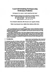
Figure 2. Two step ahead prediction with a neural network
The Neural Network’s Structure. The structure of the network has been established based on a trial and error approach. The number of input neurons has been chosen as a consequence of the simple moving average prediction. Real-time tests have shown that five values are sufficient for evaluating the performance of one parameter for a short period of time. The number of hidden layers as well as the number of neurons in each of the hidden layer was established by conducting tests. Two hidden layers can approximate any non-linear function that would describe the relationship between past and current values and future behavior. The numbers of neurons in the hidden layers are 19, and 5 respectively. Pre- and Post- Processing. Although all the monitoring parameters are numeric and thus appropriate to be passed to the network, some pre-processing and post-processing must be done. Due to the sigmoid activation function used, the output is in the range (0, 1). As a consequence, some scaling algorithm must be applied to ensure that the network’s output will be in the right range. The simplest scaling function is minimax: this finds the minimum and maximum values of a variable in all training data, and performs a linear transformation (using a shift and a scale factor) to convert the values into the target range (typically [0, 1]). Experiments
have shown that because of the wide range of the variables, the resulted predictions have a low precision. In order to improve the predictions, a different scaling approach has been implemented. Instead of finding the minimum and maximum values in all training data, the patterns are considered individually. The minimum and maximum values required for the scaling algorithm are computed as µ − σ and µ + σ respectively, where µ is the mean of the set of values in one pattern and σ is the standard deviation. Using this scaling algorithm, the accuracy of the prediction is significantly better then when using the minmax function. Training the Network. The neural network is trained using the back propagation algorithm. The patterns in the training set are selected from the historical monitoring data. If the interval between values is one minute, then a training set must contain at approximately two hours of gathered monitoring information. The historical data is provided by the Web Service client. The training patterns are chosen at run time, given that the performance of the resources can change over time. The large amount of data is divided into input and target patterns and passed to the neural network for training. The back propagation algorithm will analyze the training set a large number of times, until the network’s error will reach an acceptable level. After the neural network is trained, recent historical data is passed to the network and it produces the next value of that particular parameter. In the case of the program that runs as a background thread, the process is repeated every minute in order to predict periodically the next future value. Multiple Step Ahead Prediction. In the case of multiple step ahead prediction, the same neural network is used. After the next value in a time series is produced, the following values can be estimated by feeding the newly generated value back into the network with other previous values. Figure 2 shows an example of a two step ahead prediction and how is generated. In order to predict two steps ahead, the procedure needs the last five values. The prediction process begins at the current moment t, and is trying to predict the value at the time t + 1. The predicted value is considered correct and it is fed back into the network as an input, along with the shifted past values. The process is repeated and the network produces the predicted value for the time t + 2.
3.4
Prediction Based Meta-Scheduling Algorithm
In the case of a static scheduling approach, resources are allocated as soon as the request arrives at the Agent. When dealing with task dependencies, it is possible that some tasks will have the start time in the future, due to precedence constrains. In the case of DAG scheduling, the nodes and
edges are obtained by estimation at compile time. Based on the requirements of each tasks and available resources the start time for each task can be estimated.
Figure 3. Scheduling Framework
We present in section 2 the related work describing the latest tentative to elaborate a scheduling algorithm based on predictions. We propose a method to use the prediction component described in the last section in a distributed framework. The proposed prediction-based meta-scheduler uses the two entities model for the scheduler architecture (see figure 3). The Broker collects the users requests and the start time for each task is determined. In the case when the start time is in the future, rather than at the current moment, the Agent uses the predicted state of the system. Using this approach, an optimal scheduling solution can be achieved in a static manner. This way the much more expensive dynamic scheduling approach can be avoided. When the start time for each task is known, the resource status predictions can be used to schedule the task in a static approach. The Agent running the scheduler algorithm can use the estimated resource status to match them with the submitted tasks. The next section presents the experimental results of testing the prediction methods. The very good results for prediction methods sustains the correctness for the Step 4 from the described algorithm.
4
We will present the results of the experimental tests made for “Load10” parameter. While it is easy to implement and requires no additional overhead, its performance is marginally satisfactory. By the nature of the calculation, this algorithm produces results that are both delayed and dampened. The algorithm has a tendency to flatten local peaks as a result of the averaging function, but the result generally follows the real trends. Simple Moving Average. While it is easy to implement and requires no additional overhead, its performance is marginally satisfactory. By the nature of the calculation, this algorithm produces results that are both delayed and dampened. The algorithm has a tendency to flatten local peaks as a result of the averaging function, but the result generally follows the real trends (see figure 4).
Figure 4. Load10 real (red) and predicted (blue) values using a simple moving average
Figure 5. Load10 real (red) and predicted (blue) values using a restricted moving average
Experimental Results
In order to evaluate the accuracy of the prediction methods, a Java class has been implemented for each algorithm. The program runs as a background thread providing real time prediction for some of the most important monitoring parameters. Most of the parameters have a very instable behavior. Consequently, the predictions are rarely 100 percent accurate, but rather give a good estimate of near future behavior. In this sense, various parameters were chosen in order to test the prediction algorithm. The test benches includes parameters with high variation in time and parameters with a periodical behaviour.
Figure 6. Load10 real (red) and predicted (blue) values using a weighted moving average
Restricted Moving Average. When using this algorithm, the peak sensitivity problems persist and the restriction itself is a big source of errors, especially in the case of fast, high amplitude variations (see figure 5). In some cases
the predicted values and the real ones show opposite trends (e.g. the real value increases but the predicted value is lower than the previous one). Weighted Moving Average. Although this prediction algorithm is giving extra weight to more recent data points, the predicted values are not very accurate. The reason is that the recent past may not offer sufficient information with regard to the next value of the monitored parameter. The weighting procedure assumes that more recent data is more significant, which in some cases may not be the case, for example for rapid fluctuations (see figure 6).
been used with success in problems concerning time series prediction. They process records one at a time, and ”learn” by comparing their prediction of the record (which, at the outset, is largely arbitrary) with the known actual record. The errors from the initial prediction of the first record is fed back into the network, and used to modify the networks algorithm the second time around, and so on for many iterations. An artificial neural network provides an efficient technique for a multi-step ahead prediction. If large amount of historical data is available, a neural network is capable of discovering hidden dependencies between values at fixed time intervals without the need of other information. Load10 parameter, that shows the load of the system in the last 10 minutes, generally has large variations and its behavior is rarely repetitive, therefore the training set cannot include all the situations. According with this, the prediction achieves good performance in the case of large variations of Load10 parameter (see figure 9).
Figure 7. Load10 real (red) and predicted (blue) values using a exponential moving average with the constant
α = 0.6
Exponential Moving Average. While the performance is generally better than the one expected from a simple moving average algorithm, this method fails to produce accurate results when there is a significant difference between values at consecutive time points. Good results can be achieved by tuning the smoothing factor α, if the general behavior of the signal is known. For a completely random signal, like Load10, the results are only slightly better than the ones produced by the moving average technique, with the greatest error being produced mostly when the signal varies abruptly after a period of little or no change (see figure 7). Random Prediction. Intuitively, it can be seen that this method is well suited for predicting signals with small variations. However, the real Load5 parameter has a variation that is seldom small, meaning that the performance of this algorithm can decrease dramatically when the signal changes rapidly (see figure 8).
Figure 8. Load10 real (red) and predicted (blue) values using a random prediction
Neural Network Prediction.
Neural networks have
Figure 9. Load10 real (red) and predicted (blue) with neural network algorithm
5
Conclusions
The present paper describes several prediction methods for use in Grid and distributed system environments. Moreover, an original contribution to prediction methods, which uses a neural network has been developed, and its structure and functionality are explained. The project considers time series prediction of the status of the distributed system resources. Historical monitoring data provided by a monitoring service is used to predict one or more values into the future. The predictions are used in a meta-scheduler algorithm, improving this way the resource utilization balance. Grid computing has become an active research area due to the increasing number of scientifc applications that are both computing and data intensive. We also present the architecture developed for the prediction system in this project, along with the constituent modules. The predictions are based on historical monitoring data provided by MonALISA monitoring system. Simple prediction algorithms have been implemented and analyzed as a part of this project. The algorithms are based on classical statistical methods such as moving average and standard deviation. Some of the algorithms pre-
dict the next values as the moving average of the last five values. We used simple moving average as a prediction method, along with a restricted version of the same algorithm, weighted and exponential moving average. Random predictions based on the mean and the standard deviation are also evaluated. The resulted values were compared in time with the real measured value in order to investigate the predictions accuracy. Neural networks have been used with success in problems concerning time series prediction. An artificial neural network provides an efficient technique for a multistep ahead prediction. The behavior of resources, although sometimes periodical, is always non-linear, which makes the classic linear regression methods obsolete. If large amount of historical data is available, a neural network is capable of discovering hidden dependencies between values at fixed time intervals without the need of other information. Because of these reasons, we have also implemented a prediction system based on a neural network. The neural network predictions have been analyzed in comparison with the simple prediction algorithms. Predicting the future status of the resources composing a distributed system is important in a highly dynamic system. An optimum task scheduling based on resources state prediction will have an immediate effect on the overall balance. The selection of the system that will receive a submitted job for processing is based on the detailed information about the available resources to match the job’s requirements. The prediction based meta-scheduler can significantly improve the time necessary to schedule tasks with dependencies. Using the predictions, we have been able to state that the idle time of tasks with the start time in the future can be reduced significantly. Reducing the idle time would result in resource utilization and load balance that are close to the optimum. Future work will consider the optimization for multisteps prediction method and the possibility of tunning the scheduling algorithm.
References [1] L. Yang, J. Schopf, I. Foster, ”Conservative Scheduling: Using Predicted Variance to improve Scheduling Decisions in Dynamic Environments”, ACM/IEEE SC2003 Conference (SC’03), 2003. [2] D. Spooner, S. Jarvis, J. Cao, S. Saini, G. Nudd, ”Local grid scheduling techniques using performance prediction”, IEEE proceedings: Computer Digest Tech., Vol. 150, No. 2, March 2003. [3] I. Foster, ”Globus Toolkit Version 4: Software for Service-Oriented Systems”, IFIP International Confer-
ence on Network and Parallel Computing, SpringerVerlag LNCS 3779, pp. 2-13, 2005. [4] P. Dinda, ”A prediction-based real-time scheduling advisor”, In Proc. of the 16th International Parallel and Distributed Processing Symposium (IPDPS 2002), April 2002. [5] I.C.Legrand, H.B.Newman, R. Voicu, C.Cirstoiu, C.Grigoras, M.Toarta, C. Dobre, ”MonALISA: An Agent based, Dynamic Service System to Monitor, Control and Optimize Grid based Applications”, CHEP 2004, Interlaken, Switzerland, September 2004 [6] Y. Sugaya, H. Tatsumi, M. Kobayashi, H. Aso, ”LongTerm CPU Load Prediction System for Scheduling of Distributed Processes and its Implementation”, Proc. of the 22nd International Conference on Advanced Information Networking and Applications (aina 2008), pp. 971-977, 2008. [7] E. Heymann, M. Senar, E. Luque, M. Livny, ”Adaptive Scheduling for Master-Worker Applications on the Computational Grid”, In GRID, pp. 214-227, 2000. [8] D.P. da Silva, W. Cirne, F.V. Brasileiro, ”Trading Cycles for Information: Using Replication to Schedule Bag-of-Tasks Applications on Computational Grids”, In Proc. of EuroPar 2003, volume 2790 of Lecture Notes in Computer Science, 2003. [9] R.Wolski, N.T. Spring, J. Hayes, ”The network weather service: a distributed resource performance forecasting service for metacomputing”, In the Journal of the Future Generation Computer Systems, vol. 15, no. 5, pp. 757-768, 1999. [10] J. Brevik, D. Nurmi, R. Wolski, ”Automatic Methods for Predicting Machine Availability in Desktop Grid and Peer-to-peer Systems”, In Proc. of 4th Int. Workshop on Global and Peer-to-Peer Computing, Chicago, Illinois (USA), April 19-22, 2004. [11] F. Virili, B. Freislenben, ”Nonstationarity and data preprocessing for neural network predictions of an economic time series”, 2000 [12] J. Roman, A. Jameel, ”Backpropagation and recurrent neural networks in financial analysis of multiple stock market returns”, 1996 [13] Danilo P. Mandic, Jonathon A. Chambers, ”Recurrent Neural Networks for Prediction: Learning Algorithms, Architectures and Stability”, 2001