IEEE TRANSACTIONS ON MEDICAL IMAGING, VOL. 29, NO. 2, FEBRUARY 2010
455
Predictive Deconvolution and Hybrid Feature Selection for Computer-Aided Detection of Prostate Cancer Simona Maggio*, Alessandro Palladini, Luca De Marchi, Martino Alessandrini, Nicolò Speciale, and Guido Masetti
Abstract—Computer-aided detection (CAD) schemes are decision making support tools, useful to overcome limitations of problematic clinical procedures. Trans-rectal ultrasound image based CAD would be extremely important to support prostate cancer diagnosis. An effective approach to realize a CAD scheme for this purpose is described in this work, employing a multi-feature kernel classification model based on generalized discriminant analysis. The mutual information of feature value and tissue pathological state is used to select features essential for tissue characterization. System-dependent effects are reduced through predictive deconvolution of the acquired radio-frequency signals. A clinical study, performed on ground truth images from biopsy findings, provides a comparison of the classification model applied before and after deconvolution, showing in the latter case a significant gain in accuracy and area under the receiver operating characteristic curve. Index Terms—Computer-aided detection (CAD), hybrid feature selection, predictive deconvolution, prostate cancer, ultrasound images.
I. INTRODUCTION NE OF THE applications where computer-aided detection (CAD) tools would be extremely valuable is in recognition of prostate cancer in trans-rectal ultrasound (TRUS) images. The prostate gland is the male organ most often smitten by either benign or malignant lesions [1]. The current clinical procedure to detect cancer is based on a combination of different diagnostic tools, because none of these tools is accurate enough to be used alone. Digital rectal examination (DRE), prostate-specific antigen (PSA) evaluation, TRUS image analysis, and biopsy are all part of the medical procedure for prostate analysis. Each of these tools presents important limitations that make accurate prostate cancer detection still an unsolved problem.
O
Manuscript received July 08, 2009; revised September 30, 2009; accepted October 03, 2009. First published October 30, 2009; current version published February 03, 2010. Asterisk indicates corresponding author. *S. Maggio is with the Department of Electronics, Computer Science, and Systems (DEIS) and “E. De Castro” Advanced Research Center on Electronic Systems (ARCES), University of Bologna, 40136 Bologna, Italy (e-mail:
[email protected]). A. Palladini, L. De Marchi, M. Alessandrini, N. Speciale, and G. Masetti are with the Department of Electronics, Computer Science, and Systems (DEIS) and “E. De Castro” Advanced Research Center on Electronic Systems (ARCES), University of Bologna, 40136 Bologna, Italy. Color versions of one or more of the figures in this paper are available online at http://ieeexplore.ieee.org. Digital Object Identifier 10.1109/TMI.2009.2034517
Historically DRE has been the principal method of prostate analysis, but it is an accurate tool only to detect large and superficial lesions and it is strongly operator dependent. The first step in public screening for prostate cancer is the measurement of the blood PSA level, a glycoprotein produced almost exclusively in the epithelium of the prostate gland. Unfortunately, PSA is specific for prostate but not for cancer, since other factors such as benign prostatic hyperplasia (BPH), prostate infection, urethral instrumentation and irritation can cause increase of PSA value. In TRUS, the normal prostate gland has a homogenous, uniform echo pattern. The appearance of carcinoma on ultrasound is variable and in early stage a tumor can appear anechoic, hypoechoic, or isoechoic with respect to the surrounding normal tissues. Potential hypoechoic regions could also include BPH or even normal biological structure, thus the specificity of the TRUS images visual inspection is low. The histopathological analysis of biopsy samples is the standard for cancer detection confirmation. Ultrasounds are used in biopsy guidance, to enable sampling of all relevant areas of the prostate by means of systematic sampling protocols [2]. However, the main limitations in this procedure are due to the multifocal nature of cancer and to the sampling process. As regards patients perception of this examination, it was documented that 55% of men report physical discomfort during the biopsy. Moreover, this procedure is not completely safe, since it carries the risk of bleeding infection or even urosepsis [3]. However, since the processing of TRUS images and radio-frequency (RF) signals can highlight important characteristics of investigated tissues, the use of CAD techniques could improve the radiologist decision making process by reducing the number of unnecessary biopsies. First works on TRUS-based CAD scheme for detection of prostate cancer consist on biopsy ground truth and on analysis of rectangular regions around needle insertion points. The main characteristic of these studies is the use of textural features extracted from TRUS images to discriminate different tissues. Basset et al. [4], Huynen et al. [5], and Houston et al. [6] realized clinical studies based on the extraction of first and second order statistics textural parameters and used simple decision trees to perform classification. After these works the main trend shifted to a multifeature approach, extracting features of different nature from TRUS images and combining them to obtain higher classification performance. Schmitz et al. [7] and Scheipers et al. [8] employed textural features and spectral parameters extracted from RF data,
0278-0062/$26.00 © 2010 IEEE
456
while Feleppa et al. [9] introduced clinical data like PSA value and patient’s age in the feature vector besides spectral parameters. The classifiers used for these works (self organizing Kohonen map, neuro-fuzzy systems, artificial neural network) are more complex with respect to decision trees and define a new direction in this research field. Furthermore in these works the ground truth comes from prostatectomy and histological analysis of prostate slices and not from biopsy. The work of Mohamed and Salama [10] represents an exception since the gold standard is based on radiology visual inspection. The proposed scheme utilizes a pure textural feature vector with a support vector machine (SVM) classifier. In this case the values of sensitivity, specificity and area under receiver operating characteristic (ROC) curve are high, but they are obtained on a small ground truth. Similar performance is obtained in latest studies like the extension of Mohamed’s work [11] which includes spectral features and the study performed by Han et al. [12], where morphologic features and multiresolution textural features are employed and SVM is used as classifier. In the latter work notable values of sensibility and specificity are reported but the proposed method was only tested on malignant images, thus there is no information about its behavior in completely healthy cases. This work analyzes a cancer detection procedure which exploits a nonlinear multifeature classifier based on generalized discriminant analysis (GDA) with Gaussian kernels, and involves predictive deconvolution as preprocessing step. Since the ultrasound transducer introduces an unwanted spectral shaping of the backscattered echo signal, deconvolution is used to reduce the system dependent effects. Our aim is to investigate the ability of features extracted from deconvolved US images in discriminating pathologic tissues. This issue is analyzed in terms of a performances comparison of a nonlinear classification model trained on features extracted from US images, with and without deconvolution preprocessing. A large number of features have been extracted from US RF signal to characterize different aspects of biological tissues. The combined use of features of different nature results in more accurate tissue characterization, but requires a critical operation of feature selection to identify features highly correlated to the pathologic state of the tissue. In our approach a hybrid feature selection algorithm based on the mutual information of feature set and ground truth class is used to prune unimportant features and achieve fast computation. The ground truth used in this clinical study is based on biopsy findings and histologic analysis of some regions in the images considered suspicious by expert radiologist visual inspection. The CAD scheme proposed in this article provides high classification performances (sensitivity 90%, specificity 93%, and area under the ROC curve 95%) and was tested on a ground truth containing both benignant and malignant cases. The next section regards data preprocessing. The paper continues with a summary of the feature selection strategy, while the following sections present the classification model and the clinical study. Afterward the main experimental results are collected and compared with the methods published in literature. Conclusions and possible future perspectives are discussed in the final section.
IEEE TRANSACTIONS ON MEDICAL IMAGING, VOL. 29, NO. 2, FEBRUARY 2010
II. MATERIALS AND METHODS In this study the analyzed TRUS images are acquired by a standard US System Esaote Megas with trans-rectal transducer EC123 at sampling frequency of 50 MHz and central frequency of 7.5 MHz. Through this commercial US equipment (combined with FEMMINA [13]) it is possible to have direct access to RF echo signal. The RF signal is essential to compute some spectral parameters, useful to characterize prostate tissues. The first procedure performed on the acquired data is to remove acquisition system deterministic trends from RF signal. In order to have local information about the prostate, images of 2500 96 pixels are segmented in rectangular windows, forming a series of region of interests (ROIs). Then some features are calculated from each ROI. The choice of window size is a tradeoff between statistical significance of samples in a ROI used to compute features and the resolution of the output feature image. In this study, ROIs are rectangular windows of 101 7 pixels and of about 9 mm area. One more important step in data preparation is the compensation for system-dependent effects. In this work this problem is faced through the use of deconvolution, which is able to reduce noise and increase contrast and quality of US images. Although deconvolution is a well-known topic, its usefulness in CAD schemes was rarely explored. One of the limitations on image quality is due to the blurring effect on the back-scattered echoes produced by the transducer’s can point spread function (PSF). The acquired RF-signal be considered to be the result of the transducer’s impulse reconvolved with the tissue reflectivity function (or sponse tissue response) (1) , the deconvolution alGiven the imaging system’s output gorithm produces an estimate of the tissue response . Standard techniques for in vivo US signal deconvolution require the knowledge of system PSF and are based on regularor norm ized inverse solution of (1), obtained imposing constraints on the solution [14]. The system impulsive response in vivo can not be properly estimated on phantoms because tissues cause unpredictable phase aberration, non linearity and dispersive attenuation. A minimum phase version of system PSF can be estimated from the observed signal through homomorphic deconvolution techniques [15]. The main drawbacks of these techniques are the high sensitivity of the obtained solution from the estimated PSF, which often results in image artifacts [16], loss of information and high computational cost. Predictive deconvolution techniques that are used as standards in astronomy and geophysics are less popular in medical ultrasound. Although blind deconvolution techniques are intrinsically more limited, their choice for tissue characterization is due to several aspects: they do not require PSF estimation, they are simpler to implement and have low processing time. Furthermore, blind techniques based on linear prediction perform a local whitening of the signal, taking into account time-varying PSF, which is a realistic situation in ultrasound due to the variable focusing and pulse attenuation.
MAGGIO et al.: PREDICTIVE DECONVOLUTION AND HYBRID FEATURE SELECTION
457
TABLE I FEATURE SET
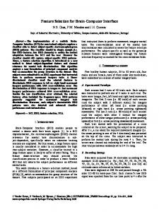
Fig. 1. Autoregressive convolutional model and predictive deconvolution iterative algorithm.
In this work, techniques like Wiener deconvolution with minimum-phase PSF estimation [17] have been compared to the linear prediction technique. We verified that Wiener technique provides over-smoothed solution and features extracted from deconvolved images are not significant for tissue characterization. On the contrary predictive deconvolution [18], based on linear prediction, is able to highlight diagnostic significance of extracted features. Predictive deconvolution uses a predictive filter to discard any and consider the unpredictable deterministic aspects from , as the repart, that is the error respect to real values of stored tissue response. Thus it is necessary to estimate the coefto predict future values of ficients of a filter (2) with an approximation of after samples. The nonpredictable part of the input signal is represented by the error
(3) The recursive least squares (RLS) algorithm [19] provides a recursive way to compute the filter which minimizes the weighted least squares error function (4) The information of new data updates the old estimate and the forgetting factor decreases the weight of data in the distant past to follow the statistical variations of the observable data. The imaging system model and corresponding deconvolution model are visualized in Fig. 1. It can be shown that the output of the deconvolution process, converges to the tissue response if the following hypotheses are fulfilled: 1) feedback hyhas an all pole transfer function and 2) random pothesis: is a white Gaussian noise process, i.e., the RF hypothesis: signal is modeled as an autoregressive process [20]. Other deconvolution algorithms such as inverse filters as in [21], or wavelet-based approaches as in [22] and [23] were considered and tested but the RLS prediction resulted to be the best compromise in terms of classification performance and computational cost.
III. FEATURE SELECTION A. Feature Set Results of recent studies show that combining features extracted from RF analysis of ultrasound signals and image-based texture parameters results in more effective classification procedures [24]. Literature about tissue characterization in ultrasound analysis provides a large amount of features of different nature which can be subdivided according to their contribution in highlighting some properties of the tissue. Parameters of statistical distributions, such as Nakagami model [25], give information about scatterer density, regularity, and amplitude. Spectral features [26] describe fluctuations of physical properties as acoustic impedance, viscosity and elasticity resulting in backscattering signals. Typical spectral parameters capture the shifting of RF signal central frequency due to attenuation. Also the wavelet coefficients of RF signal, their polynomial fitting [27] and the coherent and diffuse components obtained by signal decomposition [28] belong to spectral features group and provide important properties to type tissues. Features extraction from B-mode images aims mainly at detection of textural properties of speckle which represents the macroscopic appearance of scattering generated by tissue microstructures. Different kind of textural parameters are available in literature. Haralick [29] and Unser features [30] are both based on the gray levels distribution statistics, while Fractal features [31] rely on modeling and computation of fractal dimension. In our approach, the characteristic skills of different features are combined to define a feature set endowed with a high discriminating power between healthy and cancerous tissues. A complete feature set of all parameters mentioned before would have a huge dimensionality of about 140 attributes. For this reason, a first selection step is performed keeping for each group of features only those correlated to the ground truth class, and discarding the other ones. By doing so, the dimensionality is reduced, but synergies between different features are saved. The defined feature set is constituted by 54 features, as shown in Table I. Further information about the feature set can be found in the Appendix. B. Hybrid Feature Selection Algorithm The importance of CAD in ultrasound images is dependent on its ability to perform near real-time classification in order to give a second opinion to the physician. A large feature set dimensionality prevents the use of ultrasound images automatic
458
IEEE TRANSACTIONS ON MEDICAL IMAGING, VOL. 29, NO. 2, FEBRUARY 2010
characterization as a diagnostic decision support tool. For this reason, a further classification-oriented feature selection (FS) step is essential. FS algorithms can be roughly divided in three categories: filters, wrappers, and hybrid methods. Filters sort features according to a score measure that summarizes the importance of a feature with respect to the state of the tissue. Typically the ranking criterion can measure distance, information, dependency, or consistency between features extracted from ROIs and ROIs class (healthy or unhealthy for binary classification). Filters measures are independent on any classification algorithm. On the contrary, Wrappers sort attributes from a feature set based on performance of a classifier trained on that feature set, thus they are classifier-dependent and require larger computational cost. Hybrid methods [32] were adopted in this work to take advantage both of Filter and Wrapper models. The Filter measure is used to decide the best subset for a given cardinality, while the Wrapper mining algorithm selects the final best subset among the best subsets across different cardinalities. In particular, in our approach a mutual information hybrid FS (MIHFS) algorithm is used to rank and prune the whole feature set. Ranking measures based on distance and dependency [33] were also tested and, although most of them succeed in discarding irrelevant features, only information based measure are able to recognize and discard redundant features. In the proposed FS technique the chosen classifier-independent measure is the min-Redundant Max-Relevance (mRMR) criterion proposed by Peng et al. [34]. The mRMR measure is based on mutual information between the current feature set and class corrected with the averaged mutual information between features in the feature set. Maximizing this measure allows to define a feature set with maximum relevance, as shown by (5) and minimum redundancy, as shown by (6), where is the feature set, is the class, is the th attribute in the feature vector and is the mutual information
over-fitting on training data. Since hybrid FS algorithms require both a time-consuming search for ranking and several training iterations, in this case FLD was selected to speed up selection experiments. For the selected subset the MIHFS algorithm produces a ranked list of features which highlights their predictive skill. A previous analysis performed on ground truth samples has shown the reliability of MIHFS technique in discarding both irrelevant and redundant features. Obviously any kind of preprocessing of ultrasound images (such as deconvolution) could modify the features ranking and in general can improve or worsen the discriminating power of a feature.
(5) (6)
IV. CLASSIFICATION SYSTEM Previous studies reported that features of different nature hardly are linearly inter-correlated and that a nonlinear classification model can be able to extract valuable information from a mixed feature set and to reach higher level of accuracy [24]. On the other hand, complex model classifiers fail in preserving physical significance of features and their true dependence on pathology. In our approach a nonlinear classification model was designed and trained to discriminate between healthy and cancerous zones. The studied classifier is based on a first nonlinear feature extraction (FE) step and a second linear classification step. Empirical results on the analyzed dataset lead to choose the GDA as FE algorithm. This technique [36] uses kernel transformation to obtain a new feature space that is related to the former by a nonlinear mapping , performed on feature vector (8) The subsequent classifier is a FLD that finds the best hyperplane separating healthy and unhealthy samples of the training set. The resulting new GDA features are projected in the direction which maximizes the between-class distance and minimizes the within-class distance of samples of the mapped training set. This is a linear operation realized by simply combining mapped feature vectors (9)
MIHFS is an algorithm in two steps. The filter step and consists on ranking all features according to the mRMR measure, shown in (7), following a sequential forward selection as search technique:
where is an offset chosen to impose the same distance between centroids of the two classes of samples and hyperplane, are found by maximizing the while the weight coefficients following Fisher criterion:
(7)
(10)
MIHFS wrapper step exploits a Fisher Linear Discriminant (FLD) [35] as classifier and evaluates mining performance of the ranked feature set at increasing set size. For different cardinalities, the subset which maximizes the mRMR measure is selected and the performances of FLD trained on this subset are computed. The best cardinality and consequently the best subset is chosen as that performing the minimum FLD misclassification error. Typically the best cardinality is smaller than the maximum number of features because of classifier
In the previous expression is the between-class scatter mais the within-class scatter matrix, referred to the trix, while remapped samples of the training set. This maximization involves the computation of dot products in : such calculation can be performed efficiently by exploiting the so called kernel trick, i.e., by choosing which act like dot products in the kernel functions remapped feature space [37]. The choice of these kernel functions is crucial. In this study, different kind of kernels (namely
MAGGIO et al.: PREDICTIVE DECONVOLUTION AND HYBRID FEATURE SELECTION
Fig. 2. Comparison between linear and non linear projection on real data. Images (a) and (b) show the histograms of healthy (in dark) and unhealthy (in white) samples (five-feature vectors) after LDA and GDA projection, respectively.
Fig. 3. Classification scheme: processing steps from RF signal measurements to the derivation of final classification label.
polynomial, Gaussian, and sigmoidal kernels) were tested. The best results were obtained when a Gaussian kernel is applied. The effect of GDA feature projection is compared with the results of a simpler linear (i.e., without nonlinear mapping) discriminant analysis (LDA) in Fig. 2. In particular, the histograms in Fig. 2(a) show the distributions of healthy (in dark) and unhealthy (in white) samples after LDA projection obtained combining five features, while Fig. 2(b) shows the GDA projection of the same samples: the improvement in separation is evident. This classification system was compared with different mining techniques, both linear and nonlinear (regularized least squares, elastic net, SVM), and was selected because the computational time required for its training is significantly smaller with respect to the other tested classifiers, while providing the same accuracy. A scheme of the whole classification procedure of an ultrasound image is provided in Fig. 3. V. CLINICAL STUDY The clinical study involves 37 patients with high level of PSA and undergoing their first biopsy. The age of patients ranges from 53 to 75 years. For each patient, 10 US image frames were produced with probe held in a fixed position. Since the frame rate is about 20 frames/s, all the frames provide the same information unless for the measurement noise and micro-movements of radiologist driving the probe. Thus, in this analysis, only the first frame is considered, although the other frames can be employed in the study of stability of features and possibly to extract features averaging on several frames. The available dataset for this investigation consists of 15 benignant cases (normal and hyperplastic tissue) and 22 malignant cases (presence of adenocarcinoma). From each image, about 3000 ROIs are generated from the prostate zone and used for feature extraction. The ground truth comes from histopathological analysis from tissue samples acquired through biopsy. According to the current protocol for prostate biopsy, six needles are used to extract samples throughout the whole gland, maximizing the sampling in the peripheral zone. This proce-
459
dure cannot be without mistakes since tumors are multi-focal, and the estimated detection rate is about 89% [2]. The matching of biopsy results on TRUS images is performed by a single expert radiologist, using the exact information of needles location in the images. For each case the radiologist has matched biopsy results with precise regions on TRUS images: both pixels found to be part of cancerous zones and pixels belonging to healthy regions are selected and labeled in every zone examined through biopsy. Cancer tissue which has not been sampled during this procedure will be labeled as healthy, thus the accuracy of this process depends on the detection rate of biopsy, gold standard in this study. The pixels of the regions outlined by the radiologist are known precisely and the evaluation of features is performed over rectangular ROIs lying inside the different zones; ROIs centered on the border of two different zones are not considered in the analysis. In this study the classification model is trained on 1000 ROIs, sampled randomly from 18 TRUS images (7 benignant and 11 malignant). Training is performed through stratified 10-fold cross validation, so the classification model is generated from 900 samples and validated on the remaining 100 samples. The testing set consists of the other 19 images, completely unknown to the classification model. Classification performance is computed through ROI-based metrics on a total of 58 602 testing ROIs, where 58 286 ROIs are healthy and 316 are unhealthy. Examples of classified images and their corresponding ground truth are shown in Fig. 4. These TRUS images show the axial section of a prostatic gland without scan conversion. According to the gland anatomical shape shown in Fig. 5, the images in Fig. 4 show a prostate in the same orientation, where the superior hyperechoic boundary marks the interface between the rectum (indicated with “R” in Figs. 4 and 5) and the peripheral zone (PZ) of the prostate. The transition zone (TZ) is visible as a darker region below the peripheral zone. The gland contours are generally well defined and visible in the images. The output of a classification is visualized directly on the original TRUS image, by means of transparent colored patches located over the ROIs. Ground truth images are visualized at the left side of the set of images in Fig. 4, where healthy regions are marked in blue and cancerous regions in yellow. The classification output is shown at the right side in Fig. 4: unhealthy classified ROIs are covered in yellow, while healthy classified regions are marked in blue. Yellow and blue colors move toward white and cyan respectively when the discriminant function value is near zero, pointing out zones where classification is more difficult. A color bar is added to the side of each images set to support an easier reading of classification results. Fig. 4(a) represents a benignant case, while the others pictures show glandes affected by carcinoma. Since some false positives are always present, also in the best case and always outside biopsy region, the positive predictive value is low, but this is due to the low prevalence of unhealthy regions respect to healthy regions in a ROI-based metrics. Criteria independent on disease prevalence are employed to evaluate this clinical test (sensitivity, specificity, accuracy and area under the ROC curve) as discussed in the following section.
460
IEEE TRANSACTIONS ON MEDICAL IMAGING, VOL. 29, NO. 2, FEBRUARY 2010
Fig. 5. The picture on the left gives a schematic representation of prostate axial section with orientation inverted respect to its real anatomy. On the right a TRUS image shows the prostate gland in the same orientation.
TABLE II RANKED FEATURE SETS
sequence, MIHFS performed on the postdeconvolution feature set provides a new ranked list and a different optimal subset. FS output for the case without preprocessing and the case with predictive deconvolution are given in Table II. Listed attributes in the selected feature sets are referred to the groups described in Table I. A brief description of used features is provided in Appendix. MIHFS results show that RLS deconvolution improves the predictive skills of textural features and worsens instead the abilities of some spectral parameters. As a matter of fact, 1) deconvolution causes good speckle reduction aimed at decreasing textures dependence on the acquisition system and allows an easier edge detection, rising textural pattern significance and 2) some spectral features like the high frequency diffuse component extracted from RF signals partly lose their diagnostic value because deconvolution acts as a whitening filter, therefore these features must be computed before PSF compensation. The diagnostic significance of Nakagami features is assured in both cases, with and without predictive deconvolution. B. Classifier Performances
Fig. 4. Examples of ground truth and classified images. The letter “R” marks the location of rectum, while the color bar shows the colors used to mark zones classified as healthy (H) and unhealthy (U). The gradients indicate the discriminating function values and, thus, the colors next to the threshold between the two classes mark regions where classification is more difficult. Image (a) represents a benignant case, while (b), (c), and (d) show malignant cases.
VI. RESULTS A. Feature Selection MIHFS algorithm selects a feature subset whose cardinality is equal to 10. Feature extraction performed after deconvolution yields to different distributions of feature values. As a con-
In order to assess classifier performances, mean value and standard deviation of sensitivity (SE), specificity (SP), accuracy (Acc), and area under the ROC curve (Az) were estimated over ten different experiments, where images in the training and test set are randomly selected. In Table III performance measures related to the GDA-FLD classifier with and without RLS deconvolution preprocessing step are collected (mean value standard deviation). Each table row refers to a classifier trained on a different number of features from 5 to 54. Classification without deconvolution shows sensitivity ranging between 0.51 and 0.72, specificity and accuracy ranging between 0.89 and 0.97, and ROC area ranging between 0.87 and 0.92. Classification performances decrease as number of features increase, when more than 10 parameters are employed. This indicates an over-fitting on training data when a high number of attributes is used. The addition of predictive
MAGGIO et al.: PREDICTIVE DECONVOLUTION AND HYBRID FEATURE SELECTION
461
TABLE III CLASSIFIER PERFORMANCE
Fig. 7. Boxplots of distributions of ROC area for classification without preprocessing (In figure: Az 5 and Az 10 when using 5 and 10 features, respectively) and classification after RLS preprocessing. (In figure: Az 5 RLS and Az 10 RLS when using 5 and 10 features, respectively.)
TABLE IV PUBLISHED METHODS FOR ULTRASOUND-BASED PROSTATE TISSUE CHARACTERIZATION
Fig. 6. ROC of classification with and without RLS predictive deconvolution. (a) and (b) Performance for a 5 features and 10 features classification model, respectively.
deconvolution improves performances of 3% in terms of ROC area when 5 or 10 features are used, 1% and 4% for the case with 20 and 54 features, respectively, where the effect of overfitting is evident. In the best case classification performances after RLS preprocessing provide a value of the ROC area of 98%. These results are better visualized in Fig. 6, where ROC
curves of the two classifiers in the best case are compared when involving 5 and 10 features. The improvement is visible in the shifting of Az distributions mean value toward higher values from the case without preprocessing to the case with RLS preprocessing. Az distributions (5 and 10 features) are shown in Fig. 7 for the cases with and without RLS preprocessing. The overall result of the introduction of predictive deconvolution is an improvement of classification performances with an addition of complexity that can be negligible with respect to FE complexity. These processing times are still far from being real-time, but further work can be done to speed up the whole classification procedure, like using C implementation of spectral and textural features and defining larger “natural” regions of interest, based on textural characteristics of the prostate. The additional ROI definition step does not bring extra computational complexity, as the cost saved in FE due to the analysis of a smaller number of ROIs is more important than the supplementary cost of segmentation. Thus this step would provide a reduction of both feature generation and classification computational time. In Table IV, a summary of previously published methods for prostate tissue characterization (discussed in the introduction) is visualized in order to show research developments in computer-aided cancer detection and as a comparison with the study presented in this paper.
462
IEEE TRANSACTIONS ON MEDICAL IMAGING, VOL. 29, NO. 2, FEBRUARY 2010
VII. CONCLUSION Prostate cancer is a common disease among men and early stage detection is crucial for a successful pathology treatment. The current clinical procedure for diagnosis and grading of the disease, i.e., biopsy and histopathological images analysis, is still matter of controversy because it is invasive, dangerous and affected by errors due to the sampling process and the multi focal nature of prostate cancer. In this context, the availability of a CAD tool would be very useful to physicians to be supported in their decision and detect cancer even in its early stage. TRUS images based CAD systems can be efficient tools to perform more objective prostate cancer diagnosis reducing inter-operator variability. The use of ultrasound technology for prostate cancer detection is motivated by its minimal invasiveness and cost and, furthermore, TRUS technique is already integrated in the standard procedure for prostate examination. This study reported tissue characterization based on a multi feature approach, where spectral, statistic and textural attributes were extracted by TRUS images in the prostate zone and used for ROI classification. An hybrid feature selection algorithm exploits mutual information between features and pathologic state of ground truth tissue to reduce feature set dimensionality, discarding irrelevant or redundant attributes. In the proposed CAD scheme the resized feature set is processed by a Gaussian remapping, shifting the problem in a sub dimensional space, where linear classification is more effective. This work was also meant to explore the utility of deconvolution for classification purposes and to provide a comparison between non linear classification performance with and without deconvolution preprocessing. At this aim, a predictive deconvolution is applied to ultrasound data before FE, producing an average increase in classification performance of about 3% in terms of area under the ROC curve. The proposed classification procedure was designed and tested on a 37 images ground truth and provides a CAD system performing a highly accurate detection inside the prostate zone. The results obtained in this study are encouraging about using deconvolution in CAD schemes, but further investigations on larger datasets are necessary to assess the diagnostic significance of this model.
APPENDIX FEATURE SET A multifeature approach is used in this work based on attributes of different nature, which will be briefly described in the following paragraphs. In general, every single group of features produces several attributes, but a correlation analysis performed on each group provides a selection, shown in Table I in the column (#), indicating the selected number of attributes from a certain group. Once a output feature image is obtained, a statistical parameter, indicated in the feature name as shown in Table II, is computed on feature values in each ROI. Wavelet Transform: This feature groups the wavelet packet coefficients of the RF signal, decomposed in four bands. According to the correlation analysis only first and third bands coefficients are considered meaningful.
Polynomial Fit of Wavelet Packet Transform: The computation of this feature consists on the extraction of four bands decomposition WT coefficients of the RF signal. The second step is a fitting of the computed WT coefficients for each point of RF signal with a third order polynomial [27]. The result is a projection of the WT coefficients in a lower dimensionality space. Only the second order coefficient is considered meaningful by correlation analysis. Wavelet Decomposition: This feature consists on the decomposition of RF signal in its coherent and diffuse parts [20]. The RF signal is modeled as a sum of a diffuse component, due to the interaction of the pulse with resolvable scatterers, and a diffuse component due to the randomly located unresolvable scatterers. When a coherent component is present in time the scale-averaged wavelet power (SAP) is characterized by larger peaks, used to detect the time location of coherent scatterers through thresholding. The coherent component is then reconstructed according to the model, through superposition of Gaussian modulated sinusoids. The diffuse component is derived from difference of the RF signal and the coherent component. An inverse wavelet packet transform is applied to both coherent and diffuse signals and the coefficients in the eighth and ninth node of the packet wavelet tree are used as attributes. The generated feature set is then composed on four features, but just the mean of the third parameter, WDES Diff. Proj. n.8, is meaningful for classification purposes according to correlation analysis. The name WDES indicates the used decomposition algorithm: wavelet-based despeckling [39]. Central Frequency: This feature is an estimate of the mean central frequency of the RF signal. According to the algorithm based on amplitude spectrum magnitude (ASM), the integrated backscatter coefficient (IBS) is first evaluated as an average of the PSD of the RF signal, computed by means of FFT. Next the mean central frequency is estimated as the momentum of order 1 of RF signal PSD, i.e., it is computed as
Attenuation: This group of features is based on the main idea that slope and intercept of the linear fitting of the RF signal central frequency are measures of signal attenuation and thus of backscatter [8]. The first step to compute this feature consists on the RF signal PSD evaluation, which can be performed through several algorithms: zero crossing applied on a sliding window, FFT, fitting with an auto-regressive (AR) model of a certain order. In the last method the meaningful frequencies corresponding to non trivial maximums and minimums of the AR spectrum can be computed analytically since they only depend on the AR coefficients. A last way to compute this attenuation features is based on modified PSD whose linear trending is removed and a smoothing procedure is applied to minimize the variance of spectral slope estimation [40]. After PSD estimation the central frequency over the signal and its linear fitting are computed. The whole feature set contains 18 attributes but the correlation analysis select 13 of them, privileging computation based on AR model. In particular, in the ranked feature sets in Table II only the intercept of central frequency fitting in the case of second-order AR model estimated through Burg method
MAGGIO et al.: PREDICTIVE DECONVOLUTION AND HYBRID FEATURE SELECTION
(Intercept AR(2) burg) and the intercept of the second frequency extracted in the third-order AR model computed through a LMS procedure (Intercept2 AR(3) lmsd) are selected. B-Mode: This single attribute represents the B-mode value of the analyzed RF signal, computed through its Hilbert Transform. Nakagami: This group of features comes from a statistical model of the RF signal based on the generalized Nakagami distribution. Shape and scale parameters of Nakagami distributions estimated on the RF signal are shown to be correlated to the density and intensity of scatterers and can be computed through estimation of some RF signal statistical moments [25]. The attributes used in this work are the logarithm of the shape and scale parameters computed on the envelope of the RF signal (Nakagami logm and Nakagami logOmega). The same parameters can be extracted from the coherent and diffuse component of the RF signal. Correlation analysis selects shape and scale parameters when they are extracted from the RF signal, while only the scale parameter (Naka w Diff. Proj. n. node number, Naka w Coher. Proj. n. node number) is selected when these attributes are extracted from the RF signal diffuse and coherent component, thus this feature set contains four different attributes. Statistic: Both the mean and the variance of the pure RF signal in each ROI are considered by the correlation analysis as important attributes for diagnostic purposes. Thus, these feature set contains two different attributes. Haralick: This textural feature contains statistical attributes generated from co-occurrence matrix of the ROI in the direction of 45 [29]. Several different statistical parameters can be computed from the co-occurrence matrix in each direction, but the correlation analysis selects as meaningful features only four of them: sum of squares (Haralick Sum of Squares), correlation, entropy and average of the histogram of sum of grey levels. Unser: This feature contains statistical attributes generated from histogram of sum and difference of grey levels in the ROI [30]. Nine statistical parameters can be computed from sum and difference histogram: mean, variance, contrast, homogeneity, cluster shade, cluster prominence, energy, correlation, and entropy. These measures can be replicated for all the four angular directions (0 , 45 , 90 , and 135 ), giving a total of 36 attributes. Correlation analysis selects the following attributes: mean for the horizontal direction, correlation for the direction of 45 , mean and contrast for the vertical direction and correlation, cluster prominence, entropy and homogeneity for the direction of 135 , providing a nine attributes feature set. Fractal: This group of parameters is based on computation of progressive binarized versions of B-mode images [31], [41] obtained through ten different binary thresholding operations. Lattice of different grid size highlights the number of squares containing active pixels, expressed through the lattice size and the fractal dimension. Finally the fractal features are computed through linear regression of the number of active squares respect to the lattice size. Both slope (Alpha) and intercept (Beta) are used as features, providing 20 different fractal attributes, named Fractal(1) Alpha/Beta num attribute. A different kind of fractal feature is based on a sequence of imaginary extensions of original image toward upper and lower grey levels, considered as surfaces of a volume with a certain radius surrounding
463
the original image [42], [41]. The surface area contains information about the difference of two subsequent extended images and it is expressed through the fractal dimension and the volume radius. Choosing ten different radius values and performing a piece-wise linear regression of the surface area, the derived slopes (Alpha) and intercepts (Beta) are used as textural features. This fractal feature provides 20 more different attributes, named Fractal(2) Alpha/Beta num attribute. Correlation analysis selected seven attributes from the first group of fractal features and nine from the second group, providing a set of 16 features. ACKNOWLEDGMENT The authors would like to thank Prof. L. Masotti, University of Florence, and his group for providing the ground truth images. They also would like to thank M. Guerquin-Kern, who offered them helpful review. REFERENCES [1] J. McAninch and E. Tanagho, Smith’s General Urology., 17th ed. New York: McGraw-Hill/Appleton & Lange, 2008. [2] J. Raja, N. Ramachandran, G. Munneke, and U. Patel, “Current status of transrectal ultrasound-guided prostate biopsy in the diagnosis of prostate cancer,” Clin. Radiol., vol. 61, pp. 142–153, 2006. [3] M. Essink-Bot, H. de Koning, H. Nijs, W. Kirkels, P. V. der Maas, and F. Schroder, “Short-term effects of population-based screening for prostate cancer on health-related quality of life,” J. Nat. Cancer Inst., vol. 90, pp. 925–931, 1998. [4] O. Basset, Z. Sun, J. Mestas, and G. Gimenez, “Texture analysis of ultrasonic images of the prostate by means of co-occurrence matrix,” Ultrason. Imag., vol. 15, pp. 218–237, 1993. [5] A. Huynen, R. Giesen, J. de la Rosette, R. Aarnink, F. Debruyne, and H. Wijkstra, “Analysis of ultrasonographic prostate images for the detection of prostatic carcinoma: The automated urologic diagnostic expert system,” Ultrasound Med. ., vol. 20, no. 1, pp. 1–10, 1994. [6] A. Houston, S. Premkumar, D. Pitts, and R. Babaian, “Prostate ultrasound image analysis: Localization of cancer lesions to assist biopsy,” in Proc. 8th IEEE Symp. Computer-Based Med. Syst., 1995, pp. 94–101. [7] G. Schmitz, H. Ermert, and T. Senge, “Tissue-characterization of the prostate using radio frequency ultrasonic signals,” IEEE Trans. Ultrason., Ferroelectr., Freq. Control, vol. 46, no. 1, pp. 126–138, Jan. 1999. [8] U. Scheipers, H. Ermert, H. Garcia-Schurmann, T. Senge, and S. Philippou, “Ultrasonic multifeature tissue characterization for prostate diagnostics,” Ultrasound Med. Biol., vol. 29, no. 8, pp. 1137–1149, 2003. [9] E. Feleppa, J. Ketterling, C. Porter, and J. Gillespie, “Ultrasonic tissue type imaging (tti) for planning treatment of prostate cancer,” Proc. SPIE, vol. 5373, no. 223, 2004. [10] S. Mohamed and M. Salama, “Computer-aided diagnosis for prostate cancer using support vector machine,” Proc. SPIE, vol. 5744, no. 898, 2005. [11] S. Mohamed and M. Salama, “Prostate cancer spectral multifeature analysis using trus images,” IEEE Trans. Med. Imag., vol. 27, no. 4, pp. 548–556, Apr. 2008. [12] S. Han, H. Lee, and J. Choi, “Computer-aided prostate cancer detection using texture features and clinical features in ultrasound image,” J. Digital Imag., vol. 21, no. Suppl 1, pp. S121–33, 2008. [13] M. Scabia, E. Biagi, and L. Masotti, “Hardware and software platform for real-time processing and visualization of echographic radiofrequency signals,” IEEE Trans. Ultrason., Ferroelectr., Freq. Control, vol. 49, no. 10, pp. 1444–1452, Oct. 2002. [14] J. Ng, R. Prager, N. Kingsbury, G. Treece, and A. Gee, “Wavelet restoration of medical pulse-echo ultrasound images in an em framework,” IEEE Trans. Ultrason., Ferroelect., Freq. Contr., vol. 54, no. 3, pp. 550–568, Mar. 2007. [15] O. Michailovich and D. Adam, “Phase unwrapping for 2-D blind deconvolution of ultrasound images,” IEEE Trans. Med. Imag., vol. 23, no. 1, pp. 1–7, Jan. 2004.
464
IEEE TRANSACTIONS ON MEDICAL IMAGING, VOL. 29, NO. 2, FEBRUARY 2010
[16] H. Shin, R. Prager, J. Ng, H. Gomersall, N. Kingsbury, G. Treece, and A. Gee, “Sensitivity to point-spread function parameters in medical ultrasound image deconvolution,” Ultrasonics, vol. 49, no. 3, pp. 344–357, 2009. [17] O. V. Michailovich and D. Adam, “A novel approach to the 2-D blind deconvolution problem in medical ultrasound,” IEEE Trans. Med. Imag., vol. 24, no. 1, pp. 86–104, Jan. 2005. [18] K. Peacock and S. Treitel, “Predictive deconvolution: Theory and practice,” Geophysics, vol. 34, no. 2, pp. 155–169, 1969. [19] S. Haykin, Adaptive Filter Theory, 4th ed. Englewood Cliffs, NJ: Prentice-Hall, 2002. [20] G. Georgiou and F. Cohen, “Tissue characterization using the continuous wavelet transform, Part i: Decomposition method,” IEEE Trans. Ultrason., Ferroelectr., Freq. Control, vol. 48, no. 2, pp. 355–363, Feb. 2001. [21] L. De Marchi, A. Palladini, N. Testoni, and N. Speciale, “Blurred ultrasonic images as isi-affected signals: Joint tissue response estimation and channel tracking in the proposed paradigm,” in Proc. IEEE Ultrason. Symp., 2007, pp. 1270–1273. [22] R. Neelamani, H. Choi, and R. Baraniuk, “Forward: Fourier-wavelet regularized deconvolution for ill-conditioned systems,” IEEE Trans. Signal Process., vol. 52, no. 2, pp. 418–433, Feb. 2004. [23] S. Caporale, A. Palladini, L. D. Marchi, N. Speciale, and G. Masetti, “Wavelet-based algorithms for speckle removal from B-mode images,” in Proc. IASTED Int. Conf. Biomed. Eng., 2004, vol. 417. [24] M. Moradi, P. Mousavi, and P. Abolmaesumi, “Computer-aided diagnosis of prostate cancer with emphasis on ultrasound-based approaches: A review,” Ultrasound Med. Biol., vol. 33, no. 7, pp. 1010–1028, 2007. [25] P. Shankar, “Ultrasonic tissue characterization using a generalized Nakagami model,” IEEE Trans. Ultrason., Ferroelectr., Freq. Control, vol. 48, no. 6, pp. 1716–1720, Jun. 2001. [26] E. Feleppa, W. Fair, T. Liu, A. Kalisz, W. Gnadt, and F. Lizzi, “Two-dimensional and three-dimensional tissue-type imaging of the prostate based on ultrasonic spectrum analysis and neural network classification,” Proc. SPIE, vol. 3982, no. 152, 2000. [27] L. Masotti, E. Biagi, S. Granchi, L. Breschi, E. Magrini, and F. D. Lorenzo, “Clinical test of rules (rules: Radiofrequency ultrasonic local estimators),” in Proc. IEEE Ultrason. Symp., Aug. 2004, vol. 3, no. 23–27, pp. 2173–2176. [28] G. Georgiou, F. Cohen, C. Piccoli, F. Forsberg, and B. Goldberg, “Tissue characterization using the continuous wavelet transform. Part ii: Application on breast RF data,” IEEE Trans. Ultrason., Ferroelectr., Freq. Control, vol. 48, no. 2, pp. 363–373, 2001.
[29] R. Haralick, K. Shanmugam, and I. Dinstein, “Textural features for image classification,” IEEE Trans. Syst., Man, Cybern., vol. 3, no. 6, pp. 610–621, 1973. [30] M. Unser, “Sum and difference histograms for texture classification,” IEEE Trans. Pattern Anal. Mach. Intell., vol. 8, no. 1, pp. 118–125, Jan. 1986. [31] W. Lee, Y. Chen, and K. Hsieh, “Ultrasonic liver tissues classification by fractal feature vector based on m-band wavelet transform,” IEEE Trans. Med. Imag., vol. 22, no. 3, pp. 382–392, Mar. 2003. [32] H. Liu and L. Yu, “Toward integrating feature selection algorithms for classification and clustering,” IEEE Trans. Knowl. Data Eng., vol. 17, no. 4, pp. 491–502, Apr. 2005. [33] I. Witten and E. Frank, Tools Data Mining: Practical Machine Learning Tools and Techniques. New York: Elsevier, 2005. [34] H. Peng, F. Long, and C. Ding, “Feature selection based on mutual information: Criteria of max-dependency, max-relevance and minredundancy,” IEEE Trans. Pattern Anal. Mach. Intell., vol. 27, no. 8, pp. 1226–1238, Aug. 2005. [35] S. Theodoridis and K. Koutroumbas, Pattern Recognition. New York: Academic, 2008. [36] G. Baudat and F. Anouar, “Generalized discriminant analysis using a kernel approach,” Neural Comput., vol. 12, no. 10, pp. 2385–2404, 2000. [37] M. Aizerman, E. Braverman, and L. Rozonoer, “Theoretical foundations of the potential function method in pattern recognition learning,” Autom. Remote Contr., vol. 25, pp. 821–837, 1964. [38] R. Llobet, J. Perez-Cortes, A. Toselli, and A. Juan, “Computer-aided detection of prostate cancer,” Int. J. Med. Inform., vol. 76, pp. 547–556, 2007. [39] F. Argenti and L. Alparone, “Speckle removal from SAR images in the undecimated wavelet domain,” IEEE Trans. Geosci. Remote Sensing, vol. 40, no. 11, pp. 2363–2374, Nov. 2002. [40] D. Liu and M. Saito, “A new method for estimating the acoustic attenuation coefficient of tissue from reflected ultrasonic signals,” IEEE Trans. Med. Imag., vol. 8, no. 1, pp. 107–110, Mar. 1989. [41] T. Wagner, Handbook of Computer Vision and Applications Volume 2 Signal Processing and Pattern Recognition. New York: Academic, 1999, pp. 275–308. [42] S. Peleg, J. Naor, R. Hartley, and D. Avnir, “Multiple resolution texture analysis and classification,” IEEE Trans. Pattern Anal. Mach. Intell., vol. 68, no. 4, pp. 518–523, Jul. 1984.