for High-Performance Climate Data Analysis. Daniel Q. Duffy1, John L. ... maintains advanced data capabilities and facilities that allow researchers within and ...
Preliminary Evaluation of MapReduce for High-Performance Climate Data Analysis Daniel Q. Duffy1, John L. Schnase2, John H. Thompson1, Shawn M. Freeman3, and Thomas L. Clune3 2 Office
1 NASA Center
for Climate Simulation (NCCS) of Computational and Information Science and Technology (CISTO) 3 Software System Support Office (SSSO) NASA Goddard Space Flight Center Greenbelt, MD 20771
Abstract— MapReduce is an approach to high-performance analytics that may be useful to data intensive problems in climate research. It offers an analysis paradigm that uses clusters of computers and combines distributed storage of large data sets with parallel computation. We are particularly interested in the potential of MapReduce to speed up basic operations common to a wide range of analyses. In order to evaluate this potential, we are prototyping a series of canonical MapReduce operations over a test suite of observational and climate simulation datasets. Our initial focus has been on averaging operations over arbitrary spatial and temporal extents within Modern Era RetrospectiveAnalysis for Research and Applications (MERRA) data. Preliminary results suggest this approach can improve efficiencies within data intensive analytic workflows. Keywords-MapReduce, Hadoop, high-performance analytics I. INTRODUCTION
Our understanding of the Earth’s processes is based on a combination of observational data records and mathematical models. The size of NASA’s observational data sets is growing dramatically as new missions come online. However a potentially bigger data challenge is posed by the work of climate scientists, whose models are regularly producing data sets of hundreds of terabytes or more. The NASA Center for Climate Simulation (NCCS) provides state-of-the-art supercomputing and data services specifically designed for weather and climate research [1]. The NCCS maintains advanced data capabilities and facilities that allow researchers within and beyond NASA to create and access the enormous volume of data generated by weather and climate models. Tackling the problems of data intensive science is an inherent part of the NCCS mission. There are two major challenges posed by the data intensive nature of climate science. There is the need to provide complete lifecycle management of large-scale scientific repositories. This capability is the foundation upon which a variety of data services can be provided, from supporting active research to large-scale data federation, data publication and distribution, and archival storage. In the NCCS, we think of this aspect of our mission as climate data services. _______________________________________________________________ This work is funded by the NASA Science Mission Directorate’s High End Computing Capability (HECC) Project [2, 3].
The other data intensive challenge has to do with how these large datasets are used: data analytics — the capacity to perform useful scientific analyses over enormous quantities of data in reasonable amounts of time. In many respects this is the biggest challenge; without effective means for transforming large scientific data collections into meaningful scientific knowledge, our mission fails. MapReduce is an approach to high-performance analytics that may be useful to data intensive problems in climate research [4]. MapReduce enables distributed computing on large data sets using clusters of computers. It is an analysis paradigm that combines distributed storage and retrieval with distributed, parallel computation, allocating to the data repository analytical operations that yield reduced outputs to applications and interfaces that may reside elsewhere. The architecture thus has important networking and communications implications as well. While MapReduce has proven effective for large repositories of textual data, its use in data intensive science applications has been limited [5, 6], because many scientific data sets are inherently complex, have high dimensionality, and use binary formats. To gain a better understanding about the potential of this approach, we have been evaluating MapReduce and the Apache open-source Hadoop Distributed File System (HDFS) [7] on representative collections of observational and climate data. We have focused on a small set of canonical, early-stage analytical operations that represent a common starting point in many analysis workflows in many domains: for example, average, minimum, maximum, and standard deviation operations over a given temporal and spatial extent. In this paper, we describe our evaluation of select MapReduce attributes from these experiments, including an assessment of data preparation, ingest, and space complexities of creating repositories of the test data sets and the time and space complexities of server-side processing of canonical operations along scaled ranges of their spatiotemporal parameters. II. CLASSIC ANALYTIC WORKFLOWS Data intensive analytic workflows bridge between the largely unstructured mass of stored scientific data and the highly structured, tailored, reduced, and refined products used
by scientists in their research. In general, the initial steps of an analysis, those operations that first interact with a data repository, tend to be the most general, while data manipulations closer to the client tend to be the most specialized to the individual, to the domain, or to the science question under study. The amount of data being operated on also tends to be larger on the repository-side of the workflow, smaller toward the clientside end products.
of relevant climate parameters and have the following resolutions:
For example, the European Soil Moisture and Ocean Salinity (SMOS) [8] satellite is providing global maps of soil moisture every three days at a spatial resolution of 50km and global maps of the sea-surface salinity over an area of 200x200km. The NCCS manages a small subset of this data for SMOS scientists working at Goddard. These scientists would like to subset the data and find spatial zones around the Earth that do not change significantly over time. These zones can be used to calibrate and validate of SMOS instruments.
•
Native — 1/2 degree by 2/3 degree using model conventions.
•
Reduced — 1 1/4 degree by 1 1/4 degree, dateline-edge, pole-edge.
•
Reduced FV — 1 degree by 1 1/4 degree, using model conventions.
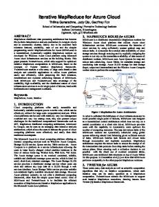
To do this now, data sets from the SMOS collection are downloaded to local work stations where they are organized, moved to NCCS computers, then analyzed using MatLab. This traditional type of workflow for large-scale data analysis severely limits the scientists and hampers their ability to look at phenomena over broader spatial extents. Importantly, this example shows how a very simple canonical operation such as finding the average value over a portion of the Earth and measuring how that value changes over time can be quite cumbersome to the scientists. III. MAPREDUCE ANALYTIC WORKFLOWS We have used the SMOS example as a foil to design a MapReduce alternative to this classic analysis scenario. MapReduce is a framework for processing highly distributable problems across huge data sets using a large number of computers (nodes). In a “map” operation the head node takes the input, partitions it into smaller sub-problems, and distributes them to data nodes. A data node may do this again in turn, leading to a multi-level tree structure. The data node processes the smaller problem, and passes the answer back to a reducer node to perform the reduction operation. In a “reduce” step, the reducer node then collects the answers to all the sub-problems and combines them in some way to form the output — the answer to the problem it was originally trying to solve. The map and reduce functions of Map-Reduce are both defined with respect to data structured in pairs [9]. For this work, we used Modern Era Retrospective-Analysis for Research and Applications (MERRA) data [10]. MERRA uses the newest version of the Goddard Earth Observing System (GEOS) Data Assimilation [11, 12] to create a reanalysis of the last 30 years of observation data. The project provides a global view of the hydrological cycle across a broad range of weather and climate time scales. Retrospective-analyses (or reanalyses) have been a critical tool in studying weather and climate variability for the last 15 years. Reanalyses blend the continuity and breadth of the output data of a numerical model with the constraints of vast quantities of observational data. The result is a long-term continuous data record. Fig. 1 shows an snapshot of MERRA data displaying the seasonal averages of temperature for the winter of 2000. The MERRA products include 2D and 3D data for a large number
Figure 1. Example of seasonal averages of temperature for the winter of 2000 taken from MERRA.
The use of MERRA data to compare with observations like those provided by SMOS is increasing in the climate community. Since MERRA data holdings are about 200 terabytes, traditional analysis approaches are simply inadequate. In this preliminary work, we have focused on the MERRA monthly means as a representative data set and computing a simple average as our canonical operation. In the remainder of this section, we describe our approach to setting up the Apache Hadoop implementation of MapReduce, how we built the file system to accommodate MERRA data, and our approach to the mapping and reducing functions. A.
Sequence Files In order to execute MapReduce operations on the MERRA data, the data first needs to be ingested into the Hadoop File System (HDFS). The MERRA data is stored within a selfdescribing NetCDF format [13] that contains both data and metadata. We considered several way to ingest the binary NetCDF data into the HDFS: •
Ingest the NetCDF Data Unchanged — Hadoop allows the flexibility for any data to be stored within the HDFS without changes. However, for binary data, Hadoop would have no knowledge of how to split a binary file into pairs. In order to map the data, a custom mapper would have to be written.
•
Custom Input Format Reader — If the data was stored in HDFS natively, then a custom input format reader would need to be created to sequence the data as it was read. This would impose a significant overhead when
reading in the data and would have to be executed each time a file is opened. •
•
File Name as the Key — Another simple method for ingesting the data into Hadoop would be to translate the name of the file to be the key and the contents of the file to be the value. Similar to above, Hadoop would not have any insight into the data itself and would not be able to intelligently place mappers in relation to the data being processed. This would likely have a large performance impact due to a significant amount of data being transferred over the network to the mapping functions. Single NetCDF File to Hadoop Sequence File — By applying our knowledge of the binary file formats, a custom sequence file can be created so that the data is logically stored as pairs within the resulting sequence file. For this case, a custom sequencer would have to be written and applied to each data file separately prior to ingesting the data into the HDFS. There would be a one-to-one mapping of the sequence file to the original data file. One benefit of this approach is that the NetCDF metadata could be preserved within the file even when the file was stored in HDFS.
B. Mapping Function The actual mapping routine was a simple filter so that only variables that matched certain criteria would be sent to the reducer. It was initially assumed that the mapper would act like a distributed search capability and only pull the pairs out of the file that matched the criteria. This turned out not to be the case, and the mapping step took a surprisingly long amount of time. The default Hadoop input file format reader opens the files and starts reading through the files for the pairs. Once it finds a pair, it reads both the key and all the values to pass that along to the mapper. In the case of the MERRA data, the values can be quite large and consume a large amount of resources to read and go through all pairs within a single file. Currently, there is no concept within Hadoop to allow for a “lazy” loading of the values. As they are accessed, the entire must be read. Initially, the mapping operator was used to try to filter out the pairs that did not match the criteria. This did not have a significant impact on performance, since the mapper is not actually the part of Hadoop that is reading the data. The mapper is just accepting data from the input file format reader.
•
Single NetCDF Variable to Hadoop Sequence File — Similar to generating new sequence files, the individual parameters within the NetCDF file could be separated into individual files. For each original NetCDF file, this would result in many sequence files (approximately 20) that would contain one and only one variable with all the values for that variable. However, this poses the problem of how to keep the linkage between the data within the individual sequence files and the metadata of the original NetCDF file.
Subsequently, we modified the default input file format reader that Hadoop uses to read the sequenced files. This routine basically opens a file and performs a simple loop to read every within the file. This routine was modified to include an accept function in order to filter the keys prior to actually reading in the values. If the filter matched the desired key, then the values are read into memory and passed to the mapper. If the filter did not match, then the values were skipped. This dramatically improved our mapping performance by about a factor of eight.
•
Single NetCDF Value to Hadoop Sequence File — In some very fine grained analyses, it might be useful to break the data up even further. The MERRA data could be broken down into a single value for each parameter at each time step and geographic location. This would result in a huge number of small files within the HDFS and bring up the issue of linkage between the data and metadata. In addition, there could be serious performance issues with this approach, as Hadoop is not designed for high performance on a large number of very small files.
C. Reduction Operation With the sequencing and mapping complete, the resulting pairs that matched the criteria to be analyzed were forwarded to the reducer. While the actual simple averaging operation was straightforward and relatively simple to set up, the reducer turned out to be more complex than expected.
We decided to create a single custom sequence file for each NetCDF file. This approach seemed to be the easiest and best solution for restructuring the data so that Hadoop could perform standard MapReduce functions while also maintaining provenance of the metadata. The single NetCDF file to Hadoop sequence file approach was selected for this work. The sequencer took each of the initial gzipped files (~235 MB) and uncompressed the file. The files were then converted into Hadoop sequence files (resulting in files as large as 500 MB or more). The conversion operation partitioned the NetCDF data by time, so that each record in the sequence file contained the name of the parameter as the key and the value of the parameter (which could have 1 to 3 spatial dimensions) at a particular time step. All of the MERRA monthly means data files were initially sequenced this way prior to ingesting into the HDFS.
Once a object has been created, a comparator is also needed to order the keys. If the data is to be grouped, a group comparator is also needed. In addition, a partitioner must be created in order to handle the partitioning of the data into groups of sorted keys. With all these components in place, Hadoop takes the pairs generated by the mappers and groups and sorts them as specified. By default, Hadoop assumes that all values that share a key will be sent to the same reducer. Hence, a single operation over a very large data set will only employ one reducer, i.e., one node. By using partitions, sets of keys to group can be created to pass these grouped keys to different reducers and parallelize the reduction operation. This may result in multiple output files so that an additional combination step may be needed to handle the consolidation of all results. D. The MapReduce Process The following describes the overall general MapReduce process that is executed for the averaging operation on the MERRA data:
1. The MERRA NetCDF files were processed into Hadoop sequence files on the HDFS Head Node. The files were read from the local MERRA directory, sequenced, and written back out to a local disk.
the reducers. This basic class just uses the field name to determine the partitions. •
2. The resulting sequence files were then ingested into the Hadoop file system with the default replica factor of three and, initially, the default block size of 64 MB. 3. The job containing the actual MapReduce operation was submitted to the Head Node to be run. 4. Along with the JobTracker, the Head Node schedules and runs the job on the cluster. Hadoop distributes all the mappers across all data nodes that contain the data to be analyzed.
B. NetCDF Sequencing Common Classes These are the shared classes used by both the sequencing application as well as the MapReduce application. They are wrapper classes used to contain the NetCDF data in a form that can be read and written to sequence files. •
NetCDFSequenceFileRecord — This is the main data class. A record contains the main field variable, along with any other variables that were associated with this field from the NetCDF file. It also stores the essential metadata associated with the variable. It contains methods that convert NetCDF variable Java objects into this record object.
•
NetCDFSequenceFileVariable — Contains the data and metadata/attributes from a NetCDF variable. This class also contains multiple convenience routines for accessing the data.
•
NetCDFSequenceFileAttribute — Attributes are metadata associated with a variable. The sequence variable class uses this class to store variable attributes.
5. On each data node, the input format reader opens up each sequence file for reading and passes all the pairs to the mapping function. 6. The mapper determines if the key matches the criteria of the given query. If so, the mapper saves the pair for delivery back to the reducer. If not, the pair is discarded. All keys and values within a file are read and analyzed by the mapper. 7. Once the mapper is done, all the pairs that match the query are sent back to the reducer. The reducer then performs the desired averaging operation on the sorted pairs to create a final pair result. 8. This final result is then stored as a sequence file within the HDFS. IV. JAVA APPLICATION This section describes the JAVA applications that perform the sequencing, mapping, and reducing of the MERRA NetCDF data. A. Common Sequence and MapReduce Classes These classes are the shared classes that would be used by any MapReduce application attempting to work with the custom NetCDF sequence files. The NetCDF sequencer also uses the composite key class when constructing the sequence files. •
NetCDFCompositeKey — This is the key object used by both the sequencer and the application. The key uses the field name and the date-time from the NetCDF file. This allows pairs to be sorted by time and grouped by field.
•
NetCDFCompositeKeyComparator — This class is used by the MapReduce framework whenever keys are compared (sorting). The comparator first compares by field name, and then by date-time.
•
NetCDFCompositeKeyGroupingComparator — This class is used by the MapReduce framework whenever grouping operations are performed (sorting). This comparator uses field name comparisons to group fields together.
•
NetCDFCompositeKeyPartitioner — This class is responsible for partitioning results from the mapper across
NetCDFRecordWriteable — This class is a customized Hadoop writeable object. This makes working with pairs from the sequence files much easier as the details for serializing/de-serializing the data are “hidden” from the main application code.
C. NetCDF Sequence Application Classes These are the main sequencing application classes. These rely on the common sequence classes to translate NetCDF files to sequence files. •
NetCDFSequenceFileGenerator — This class opens, reads, and translates input NetCDF files into Hadoop Map files (sequence files with indexing). It uses the NetCDFCompositeKey class to construct keys, and classes from the common sequence directory to construct values. The values are serialized using a library called Kryo, which efficiently packs Java objects into byte arrays.
•
NetCDFToSequenceCommandLine — This class handles parsing command line arguments (as well as config file settings) to drive the application. These arguments include input and output directory settings. The application is capable of using local files as well as files stored in HDFS for sequencing.
D. MapReduce Application The following describes the various parts of the main MapReduce application: •
Driver — The driver is what actually sets up the job, submits it, and waits for completion. The driver is driven from a configuration file for ease of use for things like being able to specify the input/output directories. It can also accept Groovy script based mappers and reducers without recompilation.
•
NetCDFAveragerMapper — Perhaps the simplest code within the entire Java application, this basically compares the current pair to the criteria for
what fields to process (in this case a simple average). Any field that does not match is rejected. Fields that are accepted are passed on to the reducer. •
NetCDFAveragerReducer — Upon receiving all the pairs from the mapper, this routine goes through the grouped and ordered pairs and performs the averaging operation based on the time period specified in the configuration file. When a period has been processed, a new pair is created and written to the context (which writes the data out to disk).
E. General Utility Classes The following classes provide functionality used throughout the code base: •
FileUtils — Provides common utility methods for working with files and directories, such as recursive searches.
•
GeneralClassLoader — Provides methods for dynamically loading code and/or scripts. This is used by the driver class to dynamically load mapper and/or reducer objects when necessary.
•
SectionedProperties/Section — Provides configuration file functionality. Sectioned property files are text-based with a simple name-value format. V. HADOOP CLUSTER
A. Local Cluster Configuration A small local cluster was built within the NCCS for testing purposes. The cluster was built out of older SuperMicro nodes, and the table below shows the details for the configuration of the different components of the nodes that made up the cluster. Component Processor Sockets Cores Per Socket Cores Per Node Main Memory Local Storage Interconnect Operating System Hadoop Version Java Version
Configuration 2.4 GHz AMD Opteron 280 2 2 4 8 GB 5 by 500 GBs Mellanox MT25208 DDR IB Ubuntu 11.04 natty 1.0 1.6.026
The five local hard drives were broken up as follows. A single hard drive was used for the operating system. Following the best practices for setting up an HDFS, the data to be stored within the file system and the local scratch for each data node were stored on different disks. Two disks each were logically striped together to make a 1 TB file system for the data (hadoop_fs) and another two disks for the local scratch space (mapred). In this way, contention between the reading of data from the hadoop_fs file system while writing to the local scratch space in mapred was eliminated.
Due to the use of older hardware, the performance of the some of the local node components was not ideal. The performance of the local disks were measured with a 16 GB write and read of a single file using a 1 MB block size to an ext3 file system. The disks were measured to have a performance of 57 MB/sec write and 108 MB/sec read. There is some concern that the local disk performance could be a limiting factor in our results. While the disk performance may not have been ideal, the network performance of the cluster was not a limiting factor. The performance of the network interfaces was measured between two representative nodes over the Single Data Rate (SDR) Infiniband connections using nuttcp [14]. The peak TCP/IP performance was measured to achieve over 6,500 Mbps. Fig. 2 shows a representative block diagram of the cluster. Two nodes were used as Head Nodes for the file system. The HDFS node, also known as the Name Node within HDFS, is the controlling node for the file system with the metadata of the file system stored within the local hadoop_fs directory. Attached to this node was a local attached array of disks that held the unsequenced MERRA data. This local MERRA repository was used to quickly sequence files to put into HDFS. The second head node, called the JobTracker node, is the node that schedules and keeps account of all running jobs. In our case, only a few jobs were run simultaneously, so the job tracker was never stressed. One could image a situation where many simultaneous jobs were running, and the JobTracker would be responsible for scheduling those jobs appropriately throughout the cluster. Eight data nodes were configured with the two local 1 TB file systems and connected to all other nodes through the Infiniband network. The data was stored within the cluster using the default replication factor of three. Head Nodes HDFS
/merra 5TB
Data Nodes
JobTracker
/hadoop_fs 1TB
Data Node 1
/hadoop_fs 1TB
Shared /home and /other via NFS across all nodes
/mapred 1TB
SDR IB
/mapred 1TB
Data Node 2
/hadoop_fs 1TB
/mapred 1TB
…
Data Node 8
/hadoop_fs 1TB
/mapred 1TB
Figure 2. Representative block diagram of the local NCCS Hadoop Cluster.
B. Word Count Example Once the cluster was installed, a simple word count was used to test the configuration. We ingested a classic text document into Hadoop 8K times resulting in a total of 34 GB of
A simple word count was executed on the cluster using 2, 4, and 8 data nodes. The following table shows the results across the three different tests. Number of Nodes 2 4 8
Timing (seconds) 6,336.3 3.227.0 1.642.3
Speedup 1.0 1.96 3.86
It can be seen from the table that the Hadoop cluster is working as expected. As the number of data nodes used is increased from 2 to 8, an almost perfect speed up of the word count was achieved. VI. ANALYZING MERRA DATA As described above, the entire set of MERRA monthly means was sequenced and ingested into the HDFS. The initial zipped monthly means encompassed approximately 181 gigabytes of data. Once uncompressed, the data volume grew to over 300 gigabytes. Upon sequencing and ingesting the data into the HDFS, this translated into about 1 TB of total data stored within the HDFS when accounting for the triplication of the data. Initially, the default block size of HDFS was used to ingest the data. After subsequent discussions about the potential performance impact occurred when data has to be passed between data nodes in the mapping step of the MapReduce application, the performance of different sized data blocks was explored. The following table shows the timing in seconds for a single MapReduce operation to average the a single parameter (surface pressure) on the NPANA 3D subset of the MERRA data. The block sizes were chosen to start from the default block size of 64 MB and roughly double each time to a point where the block size at 640 MB was larger than the biggest monthly means file. Years 1 10 20 32
64 MB (secs) 131 969 1,897 3,053
128 MB (secs) 85 510 985 1,570
320 MB (secs) 53 200 360 553
640 MB (secs) 37 80 128 187
It is clear from the table that the different block sizes have a dramatic affect on the performance of the application. In the 640 MB configuration, every sequence file is guaranteed NOT to be split between data nodes. Therefore, all the data within a file that a mapper needs is contained on that node and no data is being sent across the network between nodes. Even with the very high speed network connection of the single data rate Infiniband, there is a 20x speedup when analyz-
ing all 32 years of MERRA data using the 640 MB block size as compared to the default HDFS block size of 64 MB. Care must be taken when analyzing the best way to not only sequence but to layout the data within the HDFS for good performance. Often times, a simple operation is performed on a subset of the entire MERRA data, such as only looking at the time average of a parameter over a single year. Fig. 3 shows just such an example. Using the NPANA 3D data set, one to eight years of data were analyzed to produce a global average of surface temperature for each year. When running a single year of data, only a single job is being run across the HDFS and only a single reducer is used. As we scale up from one to eight years of data begin analyzed concurrently, then additional reducers equal to the number of years being processed are utilized.
Average of Individual Years - NPANA Concurrent
Serial
600 500
Time (seconds)
data stored within the file system. The default replication number of 3 along with the default 64 MB block size were used for these tests.
400 300 200 100 0 1
2
3
4
5
6
7
8
Number of Years Processed
Figure 3. Timings for reducing 1 to 8 years of data simultaneously showing the concurrent or parallel processing time and the serial times.
The figure shows an increase in the time of analysis of one year of data which takes ~35 seconds to eight years of data taking ~87 seconds to complete. The timing for computing all eight years of data serially is ~542 seconds. While this is not perfect speedup, it definitely shows the power of the distributed computing capability within a Hadoop file system using MapReduce. VII. CONCLUSION Our use of MapReduce on a representative set of climate data has shown potential. While MapReduce and Hadoop appear to be deceptively simple at first glance, our work has also shown that care needs to be taken with ingesting data within HDFS and understanding how the data should be laid out. Significant performance improvements can be made through a better understanding of the data layout and how the MapReduce application interacts with the data. In addition to continuing to work on the local cluster, the NCCS is exploring the use of MapReduce as a service within clouds like Amazon, looking at additional capabilities like Twister from the University of Indiana [15], and even integrating HDFS with a virtualized climate data service [16].
With the wide spread employment of these technologies throughout the commercial industry and the interests within the open-source communities, the capabilities of MapReduce and Hadoop will continue to grow and mature. The use of these types of technologies for large scale data analyses has the potential to greatly enhance our understanding of the Earth’s climate. ACKNOWLEDGEMENTS We thank Tsengdar Lee, Mike Little, and Phil Webster for their encouragement and contributions to this effort. Ed Kim and Mike Theriot provided crucial advice about the SMOS mission. Kirk Hunter provided invaluable technical support building the Hadoop clusters. REFERENCES [1] [2] [3] [4]
[5] [6] [7] [8] [9] [10] [11] [12] [13] [14] [15] [16]
NASA Center for Climate Simulation (NCCS), http://www.nccs.nasa. NASA Science Mission Directorate (SMD), http://science.nasa.gov/. NASA High End Computing Capability (HECC) Project, http://www.nasa.nasa.gov/hecc/. J. Dean and S. Ghemawat, MapReduce: Simplified Data Processing on Large Clusters, Google, Inc., http://research.google.com/archive/mapreduce.html. J. Buck, et al., SciHadoop: Array-based Query Processing in Hadoop, UC Santa Cruz, https://systems.soe.ucsc.edu/node/439. C. Ranger, et al., Evaluating MapReduce for Multi-core and Multiprocessor Systems, Computer Systems Laboratory, Stanford University. Apache Hadoop Distributed File System (HDFS), http://hadoop.apache.org/. Soil Moisture and Ocean Salinity (SMOS) Satellite, http://www.esa.int/SPECIALS/smos/index.html. MapReduce, http://en.wikipedia.org/wiki/MapReduce. Modern Era Retrospective-Analysis for Research and Applications (MERRA), http://gmao/gsfc.nasa.gov/merra. Goddard Earth Observing System (GEOS), http://gmao.gsfc.nasa.gov/systems/geso5. Global Modeling and Assimilation Office (GMAO), http://gmao.gsfc.nasa.gov/. Network Common Data Form (NetCDF), http://www.unidata.ucar.edu/software/netcdf. Network testing benchmark created by Bill Fink at NASA Goddard Space Flight Center, http://lcp.nr.navy.mil/nuttcp. Iterative MapReduce from the University of Indiana, http://www.iterativemapreduce.org. J. Schnase, et al., The Virtual Climate Data Server (vCDS): An iRODSBased Data Management Software Appliance Supporting Climate Data Services and Virtualization-as-a-Service in the NASA Center for Climate Simulation, 2012 iRODS Users Group Meeting, in review.