Preliminary Results in Blind Equalization with Neural Networks-Based

Preliminary Results in Blind Equalization with Neural Networks-Based Prediction C.C. Cavalcante(1) , J.C.M. Mota(2) , B. Dorizzi(3) , J.R. Montalvão Filho(3,4) (1) Univ. Federal do Ceará, Campus do Pici, CP 6001, CEP 60455-760, Fortaleza - Brasil, [email protected] (2) Univ. Federal do Ceará, Campus do Pici, CP 6001, CEP 60455-760, Fortaleza - Brasil, [email protected] (3) Institut National des Télécomm, 9, rue Charles Fourier, 91011 Evry-France, [email protected] (4) Universidade Tiradentes, Rua Lagarto, 264, CEP 49010-390, Aracaju - Brasil, [email protected]

Abstract - A nonlinear predictive technique for blind equalization in digital communication systems is studied in this paper. Considering the nonlinearity in the filter structure, we study prediction as a classification problem and an artificial neural network (NN) is used as a nonlinear predictor that tries to interpolate the channel states to provide correct data equalization. In this paper we analyze the performance with forward prediction and the preliminary results point to a good performance on channel with intersymbol interference (ISI). 1. INTRODUCTION The adaptive equalization problem consists on the usage of an adaptive filtering process, with a required training period, in sight of recovering a transmitted sequence and to combat the intersymbol interference inherent to certain channels. Blind adaptive equalization can be used on the digital communication systems with dispersive channels, where it is not possible to realize the learning procedure on the receiver over an acquisition period. In this case, blind synchronous adaptive equalization strategies provides nonlinearity in the signal processing in order to recover the transmitted symbols. This is supported by the optimum bayesian estimator [1]. In general, the blind synchronous adaptive equalization strategies based on a filtering process using a transversal structure, have the nonlinearity on the cost function to be minimized. This is the case of the Godard's algorithm [3] and Shalvi-Weinstein [2]. Considering the robustness of these algorithms on the cases of non-minimum phase channels with no poles, their performances are very affected by the channel characteristics. However, some strategies may also have nonlinearity on the filter structure. This can result in a higher robustness to the noise and to the channel distortion. In this case we can also obtain good performance in channels where the zeros are over the unit circle except for the points z = ± 1 [4]. The

decision feedback equalizer (DFE) [5] and the amplitude and phase equalizer [6] are examples of robust nonlinear structures in the adaptive blind equalization strategies. When we consider the transmitted symbols to be uncorrelated, it is possible to deal with the blind equalization problem by means of a nonlinear prediction [6]. In [10] we used successfully an equalizer based on prediction using neural networks for minimum phase recursive channel with high distortion. In our work, we present a robust new structure of nonlinear blind equalization for NMP channels, based on prediction using neural networks. In section 2, we present some aspects of prediction and equalization techniques. In section 3 we describe some aspects of the use of nonlinear structures for adaptive channel equalization and section 4 shows some simulation results. The conclusions are presented in the last part of this paper. 2. PREDICTION AND EQUALIZATION Figure 1 depicts the scheme of the digital communication system using the blind equalizer as an error prediction filter. The emitted data sequence a(n) belongs to a finite alphabet, and in this paper we will consider the symbols taken from the set {±1}, forming an i.i.d. sequence. The noise b(n) is the additive gaussian noise, x'(n)=[x’(n) x’(n-1) … x’(n-M+1)] is the sequence of states provided by the channel, x(n) = x'(n) + b(n) is the receiver input and xˆ(n) is the estimated channel states provided by the predictor. The AGC (Automatic Gain Control) is used to recover the power of the symbol to the desired level and â(n) is the estimated transmitted sequence. The channel is modeled as a FIR filter with the following transfer function: H (z) =

nh −1

∑h z

−i

i

i =0

where hi is the channel impulse response and nh is its length.

a(n)

Channel

x'(n)

x(n)

e(n)

+

z-1

â(n)

such case, the difference between the predicted x(n and the actual one is the “innovation”.

-

^ x(n)

b(n)

y(n)

AGC

f (•) =

Predictor

1 − e − (•)

(1)

1 + e − (• )

Figure 1: Scheme of the digital communication system using an error prediction filter x(n)

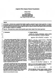
The results of the prediction error filter (PEF) used as a blind equalizer depend on uncorrelated data hypothesis about the transmitted sequence. In this case, if we use the power minimization criterion of signal error e(n) = x(n) − xˆ (n) and the linear PEF, the equalization is obtained after the AGC in a minimum phase channel [1,6]. But, this criterion does not work well with linear PEFs with nonminimum phase channels (NMP) [6]. In this paper, we consider nonlinear forward prediction and the estimated symbol is a function of the past samples of x(n) that considers in the error prediction filter composition. This can be written as: xˆ (n) = f (x(n − 1)) . The function f depends on the predictor structure and provides an approximated interpolation surface which takes into account the last channel outputs in order to estimate the current output x(n). The interpolation surface can be very complex, depending on the channel and generated intersymbol interference, and a linear structure may not be suitable to provide an acceptable performance.

In this work we use a nonlinear predictive structure based on NN to learn the NMP channel behavior. Once it is done, the structure proposed can provide information about data to remove the ISI. Naturally, NN provides a nonlinear surface of interpolation, and the output of a neuron of NN is a function written as:  Neuroni = f   

 + θ i ( n)   

M

∑

wij1 (n) xi (n)

j =1

And the neural network output is a linear combination of the neurons outputs given by: L

Net =

θi

∑ w Neuron 2 i

i

i =1

where the vector xi are the inputs, wij are the synaptic weights, the θi are the neurons bias, L is the number of neurons and f is the neuron activation function. The activation function has a characteristic of saturation and we have chosen the sigmoid tangents, described in Equation 1, due to the symmetry of the transmitted sequence. Figure 2, illustrates a possible interpolation effect corresponding to one input neural predictor. In

x(n-1) a(n) = +1 a(n) = -1

Figure 2: Interpolation surface with bias and neuron activation function. This characteristic of saturation provides a higher robustness to the noise that is not observed in the linear model. In this case, the noise is amplified when the number of filter coefficients increases. Figure 3 shows the neural network structure used as the predictor device.

w 1i,j

f

θ1

x(n-1)

3. NONLINEAR PREDICTOR

Interpolation Surface

Neuron Activation Function

w 2i

f x(n-2)

Σ

θ2

... f

x(n-M)

θ.3 .

.

f

θL

Figure 3: Neural network structure used as a predictor In this work the synaptic weights were determined through adaptive training by the back-propagation algorithm[9]. The algorithm structure is described below. . Back-Propagation Algorithm 1. Initialization of the synaptic weights 2. Inputs are shown to the neural network 3. Forward computation (computing the network output) 4. Error computation (x(n) - Net) 5. Backward propagation (computed error is propagated from the end to the beginning updating the synaptic weights and bias). The computing of the factor that updates the weights is a function of the derivative of the neuron activation function and a step factor called learning

rate that controls the speed rate of the weights coefficients. Generally, the determination of the neural network architecture is a very difficult problem. The number L of neurons depends on both channel and predictor order. For instance if there is only one nonlinear predictor input, no more than L = 2N neurons are needed to predict the inherent redundancy x(n). The backpropagation algorithm is based on the mean square error minimization. The error (e(n)) that feeds the NN to adjust the coefficients has minimum power. So, it is necessary to normalize it to recover the same power level of the transmitted data. In the case of the decided symbols, their power is recovered by the AGC which has the following algorithm of adjustment:

For reasons of better visualization we used only two dimensions. We used a normalization of the estimated states to the channel states variance to recover the original power of the states. This normalization factor can be written as the following ratio: σx σ xˆ Where σ x and σ xˆ are the standard deviations of the channel states and estimated ones, respectively.

G (n + 1) = G (n) + λ (σ a2 − y 2 ) AGC = G (n + 1) where λ and σ a2 are, respectively, the step factor of the AGC algorithm and the variance of the transmitted data, G is a constant. 4. SIMULATION STUDY Figure 4: Time-evaluation diagram (weak ISI) The simulation study was done using channels with strong and weak ISI, the noise in these cases were considered null to recover the channel states, and with that, study the equalization by the extraction of the dispersion provided by the channel, for the timeevaluation diagram the signal-noise ratio used was 17 dB. The finite NMP channel impulse response with weak ISI is given by the following equation:

H ( z ) = 0.1 + z −1 + 0.1z −2 We used the following steps on simulating the neural network: training with the back-propagation algorithm, after that using the coefficients reached by the NN, we started the test period and validation period with a new set of samples in both. For the weak ISI case, we used a NN with only one layer, 3 inputs (3 past samples of the channel states), 4 neurons and one output with a learning rate of 0.001. For the strong ISI case, the same number of inputs and neurons were used with a learning rate of 0.035. Then, NN has a very low complexity for both cases. The initialization of the synaptic weights were done with random numbers belonging to the interval [0,1]. The Figure 4 shows the time evolution of the signal y(n). We can observe that the equalization is reached quickly. To verify the behavior of the NN, we used the analyze by the plot of x(n-1) versus x(n). This diagram shows the behavior of the channel and estimated states with the influence of the past samples.

Figure 5: Plot of x(n-1) versus x(n) (weak ISI) The balls (o) are the channel states and the crosses (x) are the estimated states, provided by the NN. We can observe that the NN searches the channel states trying to remove completely the interference provided by the channel. For the strong ISI case the channel impulse response considered is given by:

H ( z ) = 0.4 + z −1 + 0.4 z −2 The Figure 6 shows the time-evaluation diagram of the NN over the channel.

Figure 6: Time-evaluation diagram (strong ISI) It is shown the convergence to the desired power level, as well an extra difficulty to track and a higher dispersion over the real level. The Figure 7 shows the phase space diagram to the same case, using the normalization factor. It is possible to see a convergence to the channel states from the NN. To compare the performance between the used structure with classical ones, we used the merit figure of Symbol Error Rate (SER) in several signal-noise ratio. The other structure of blind equalization was a linear one (transversal filter) using the classical “Constant Modulus Algorithm” (CMA) [1]. This algorithm is largely adopted industrially nowadays [11]. To specify the length of the transversal filter, we used the same number of inputs in the predictor. In both cases for the CMA, were used 3 taps for the transversal filter used as equalizer, and a step factor equals to 0.001. We can observe, in Figures 8 and 9, that the nonlinear structure has a better performance than the CMA.

Figure 8: Nonlinear predictor and CMA performance (weak ISI)

Figure 9: Nonlinear predictor and CMA performance (strong ISI)

5. CONCLUSIONS AND FUTURE WORKS The preliminary equalization results obtained using NN predictor with low complexity point to good performance. Some results with the symbol-error rate (SER) evaluation are encouraging. We are studying some complexity aspects on NN architecture. We intend to use this technique in mobile radio channels in confronting with the performance of others equalization techniques using nonlinear prediction. The use of a linear predictor to initialize the NN network, trying to reduce the learning time, is getting in work. 6. ACKNOWLEDGEMENTS

Figure 7: : Plot of x(n-1) versus x(n) (strong ISI) The crosses (x) are the estimated states, provided by the NN. And the balls (o) are the channel states.

The authors would like Mr. W. M. de Souza Jr by his remarks. We would also like to thank PET/CAPES and CNPq/SFERE by the partial financial support. 7. REFERENCES [1] HAYKIN, SIMON. Adaptive Filter Theory. 3rd Edition. Prentice-Hall International, 1996. [2] SHALVI, O. ET WEINSTEIN, E. "New criteria for blind deconvolution of non minimum phase

systems", IEEE Trans. on Inform. Theory, 36, pp.312-321. 1990. [3] GODARD, D. N. “Self-recovering equalization and carrier tracking in a two-dimensional data communication system (channels)”, IEEE Trans. on Comm., vol COM-28, pp 1867-1875, 1980. [4] J.R.MONTALVÃO, J.C.M.MOTA AND B.DORIZZI, "Some theoretical Limits of Efficiency of Linear and Nonlinear Equalizers", Submitted in Journal of Telecommunication Brazilian Society, Brazil, 1998 [5] AUSTIN, M.E. "Decision-feedback equalization for digital communication over dispersive channels" Tech. Rep. 437, MIT Lincoln Laboratory, Lexington, Mass. 1967 [6] MACCHI, O. "L’égalisation numérique en communications" Annales des Télécomm. 53, no 1-2, pp 39-58,1998. [7] J.R.MONTALVÃO F., J.C.M.MOTA, B.DORIZZI, C.C.CAVALCANTE. “Reducing Bayes Equalizer Complexity: A New Approach for Clusters Determination”, ITS'98, São Paulo, Brazil. [8] MULGREW, B. "Applying Radial Basis Functions", IEEE Signal Processing Magazine, V. 13, No. 2, pp 50-65, March 1996. [9] HAYKIN, SIMON. Neural Networks: A Comprehensive Foundation. Ed. Macmillan, 1994 [10] CAVALCANTE, C.C., MOTA, J.C.M., DORIZZI, B., MONTALVÃO FILHO AND SOUSA, C.P. “Uma Estrutura Não-Linear como Dispositivo de Predição: Uma Nova Maneira de Equalização Cega”, SBRN’98, Belo Horizonte-MG, Brazil. [11] TREICHLER, J.R., LARIMORE, M.G. AND HARP, J.C. “Practical Bind Demodulators for HigherOrder QAM Signals”, IEEE Proceedings, V. 86, No. 10, October 1998.