Probabilistic and statistical thinking

ON OUTLIERS, STATISTICAL RISKS, AND A RESAMPLING APPROACH TOWARDS STATISTICAL INFERENCE Manfred Borovcnik, University of Klagenfurt, Austria This paper is on theoretical issues dealing with interrelations between data analysis and procedures of statistical inference. On the one hand it reinforces a probabilistic interpretation of results of data analysis by a discussion of rules for detecting outliers in data sets. To prepare data, or to clean from foreign data sources, or to clear from confounding factors, rules for the detection of outliers are applied. Any rule for outliers faces the problem that a suspicious datum might yet belong to the population and should therefore not be removed. Any rule for outliers has to be defined by some scale; a range of usual values is derived from a given data set, and a value not inside this range might be discarded as outlier. Always is a risk attached to such a procedure, a risk of eliminating a datum despite the fact it belongs to the parent population. Clearly, such a risk has to be interpreted probabilistically. On the other hand, e.g. the procedure of confidence intervals for a parameter (derived from a data set) signifies the usual range of values for the parameter in question. In the usual approach towards confidence intervals, the probability distribution for (the pivot variable, which allows determining) the confidence intervals is based on theoretical assumptions. By simulating these assumptions (which is usually done), the successive realizations of the intervals may be simulated. However, the analogy to the outlier context above is somehow lost. More recently, the resampling approach towards inferential statistics allows to make more and direct use of the analogy to the outlier context: The primary sample is re-sampled repeatedly calculating always a new value for the estimator thus establishing an empirical data set for the estimator, which in due course may be analysed for outliers. Any rule to detect outliers in this distribution of the estimator may be interpreted as a confidence interval for the parameter in question; outliers are simply those values not in the confidence interval. While the paper is philosophical per se, it may have implications on the question of how to design teaching units in statistics. The author’s own teaching experience is promising: somehow it becomes much easier to compute confidence intervals; it becomes much more direct how to interpret calculated intervals. 1 Screening of data – checking for inconsistencies, errors, and extreme values There are several reasons to check for data whether they are extreme or not. One is to check for errors in the data (for whatever cause). Another reason is to check whether assumptions (e.g. normality of distribution) are fulfilled for further statistical Paper presented at CERME 5 in Larnaca, February 2007

1

investigations. Still another reason is to interpret data descriptively, i.e. to judge whether a datum is extremely high or low compared to the bulk of the other data, which might lead to specific interpretations about the subject behind (“is highly talented”; or “has to be investigated for specific causes”, etc). Formal rules to undergo this task and the reasons why such an inspection might be applied are discussed here. Maintenance of data The phase prior to the analysis of data is signified to “produce” data free of errors, which fit to the assumptions needed for statistical procedures planned to apply. In analysing data, a preliminary step is to plan carefully how to get data so that they help answering the problem in question. After the data are collected, data screening starts not only preparing an exploratory approach to the questions but also primarily to clean the data of inconsistencies and errors. Are there blunders in recording the data, either due to measurement errors, or to editing errors, etc? ‘Is the observation unit really a member of the target population’ is another important issue to clarify. There are contextual examinations and checks for internal consistencies e.g. if a person’s pattern of answers to various items is plausible, or if it is an indication of unreliable answering behaviour (exaggerating, or even lying). Besides such contextual verifications there are also criteria to check for single variables whether some values are extremely high (low). These checks might be by visual judgment from raw data or from first diagrams. Formal rules to check for outliers Two well known rules to judge whether a datum is an outlier or not are presented and compared, the sigma rules and the quantile intervals. In either case, an interval is calculated on base of given data and the specific datum is judged to be a “candidate outlier” if it lies outside this interval. The usual rule to test for outliers is the so-called sigma rule, a long standing though sound rule: Calculate mean and standard deviation (sd) of the data and check if a suspicious value lies in the interval (mean plus or minus 3 times sd) – if not inside, the value might be declared to be an outlier and discarded from the data set. For values being outside the 2-sigma interval, a check of the appending object might well be advisable; see Fig. 1a. The rule is formally applied and does not investigate the reason why this value is so extreme (i.e. if it is due to an error, or if the appending object does not belong to the target population). A modern variant of the sigma rule is the quantile interval: First calculate the lower 2.5% and the upper 97.5% quantiles; then check whether the value in question lies in the interval formed by these quantiles, see Fig. 1b with a boxplot of the data indirectly showing the quantile intervals (25, 75%) and (2.5, 97.5%). Tukey (1977) and followers would calculate so-called inner and outer fences, which are not open to a fixed percentage interpretation because the fences are different from quantiles.

Paper presented at CERME 5 in Larnaca, February 2007

2

The quantile interval has the advantage that the suspicious value has hardly any influence on the calculation of the interval and therefore the judgement of the suspicious value whether it is extreme or not, is done by a ‘scale’ nearly independent of this value in question. This value, however, influences the calculation of sd by much making the 3 sigma interval much broader which in turn might affect the ’extreme’ judgement decisively (sometimes it is suggested that sd is calculated without the suspicious value to make this test more sensitive). Another advantage of quantile intervals is its easier interpretation. While the percentage of data lying outside the sigma intervals varies from one to another data set (it is roughly 5% respectively 0.3% for the 2- and 3- sigma interval for the normal distribution where the rule comes from), quantile intervals always have a fixed percentage of data outside (and within). This is the reason why this author leaves the Tukey tradition of fences behind as Tukey fences only indirectly reveal percentages by referring to the normal distribution. Other authors like Christie (2004) use quantile intervals somehow to approximate 2-sigma rules, which subsequently will be interpreted as confidence intervals (see section 3). However, the latter reason in favour of quantile intervals may be interpreted also as disadvantage, as every data set has (even a fixed percentage of) “extreme values” – one should better say “candidate for extreme value” if a datum is not within the specified quantile interval and leave the further steps open to a specific investigation for that datum. Detect sources of interference – produce homogeneous data Data contamination may be due to single outliers, or due to another source of data influencing the symmetry of the distribution, which may cause deviations from assumptions for further statistical analyses, or simply may reflect error sources in the data generation, which in turn might impede an easy interpretation of results. One standard tool to detect such deviations is to check the shape of a distribution by diagrams like histograms or boxplots; another tool is to apply sigma rules or quantile intervals. This author suggests a combined rule, which is implicitly contained in boxplots but could also be integrated into histograms: split of the data into a central region, an outer region of usual values, and a region of candidates of extreme values. The final decision of a single datum to be an outlier is attached with a risk of being wrong as it could yet belong to the target population. For the interpretation of data based on descriptive techniques, also skewness and kurtosis is calculated. These parameters allow comparing the distribution of data with the normal distribution – is it skewed in comparison to the symmetric normal, is it too flat or too bumped up in the middle in comparison to the normal? Does the distribution (as indicated by histograms) show two peaks resembling the circumstance that in fact the population to be investigated consists of two distinct subgroups and the analysis should be done separately for the two groups?

Paper presented at CERME 5 in Larnaca, February 2007

3

One of the consequences of marked skewness is that sigma rules and quantile rules lead to considerably different intervals (sigma rules implicitly assume a symmetric distribution). The target of data ‘cleaning’ is to detect sources of interference, which might confound the final results and the conclusions derived from them. Producing homogenous sources of data (getting rid of confounding factors) is valuable for a more direct interpretation of the final results. The key question for a suspicious datum is:  Does the value belong to the (target) population, or does it belong to another population? As a technical device to check for this question, the sigma rules or the quantile intervals serve our purpose. The formal rules are sustained by diagrams: It is helpful to amend the histogram of data by the sigma intervals (mean plus minus k times sigma) in different colours: green for centre data (k = 1), grey for inconspicuous data (in the interval with k = 2 but not being in the centre), and red for suspicious data (outside k = 2) being worth for an inspection whether they are outliers or not; see Fig. 1a. The quantile intervals are better known as boxplot, in which a box signifies the central data (the central 50% between the 25 and 75% quantiles), and lines (the socalled whiskers) indicate the still inconspicuous data (e.g. between 2.5 and 97.5% quantiles but not in the central box); see Fig. 1b. And individual points, which are labelled to reveal the appending objects’ identity, usually represent the rest of the data.

Fig. 1a: Histograms with labels for the sigma regions

Fig. 1b: Boxplot with quantile regions and labels for suspicious data The final check of such data in the ‘red’ region is by going back to the data sources including the object itself and its context. A procedure which is especially supported by the boxplot where points outside the whiskers are labelled revealing their identity

Paper presented at CERME 5 in Larnaca, February 2007

4

(as they have to be checked by context, they cannot remain anonymously for the while; this procedure was already used by Tukey 1977 but seems to have been not so widely used more recently). Always there is (at least) two possibilities for a specific value:  The value is an outlier due to errors  The value belongs to an object which is not a member of the target population In either case the datum has to be eliminated. Even if the action is the same in both cases, the reason for it is completely different. The main drawback of such a decision, however, is that it might be wrong. In both cases we take a risk: It could well be that the value is free of errors, and its corresponding object truly belongs to the population. Usually the discussion of such a risk is cursory; here the author tries to exploit it to a deeper extent by relating it to games of prediction in the subsequent section. We will see an adequate interpretation for that risk in the prediction games of the next section. This risk will be the hinge between the interpretation of outlier rules and confidence intervals in section 3. 2 Different games of prediction Applying the 2-sigma rule or the analogue quantile interval rule (2.5%, 97.5% quantile) might lead to the decision to discard a datum as outlier, if the datum is not within that interval. The decision is attached with a risk of 5%. To illustrate matters, to facilitate an interpretation of such a quantity, various prediction games are introduced. The derived intervals are interpreted as prediction intervals, to predict a (fictitious) next outcome of the same data, or of a datum of the same data generation process. Herewith, the static 5% fraction of a given data set evolves into the risk of the prediction to be wrong. The risk figure reveals its inherent probabilistic character by this analogy. Similar prediction games are used to facilitate the interpretation of (linear) regression and the determination coefficient as a quantity to measure the goodness of fit of a regression function in the analysis of dependence relations between two variables. Information as it is contained in the given data set may be summarized by its mean and standard deviation, or by quantiles. These parameters have a static, descriptive meaning and a dynamic, prognostic power for future events as well. Example 1: Intervals for e.g. the prevalence of opinion A are easily communicable. E.g. among students the percentage of A lies between 12% and 42% (be it the ends of the 2 sigma interval or be it the 2.5% and 97.5% quantiles of the data): immediately one would answer, that the available information is quite imprecise. On the other hand, an interval of 35 to 39% resembles a high degree of precision. The related power, or from the reverse viewpoint, the related risk of such statements is best illustrated by the prediction games introduced.

Paper presented at CERME 5 in Larnaca, February 2007

5

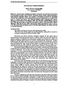
Prediction of single values of the same data set The simplest way to introduce a prediction game is to calculate a prediction interval from the given data set and then try to predict the value of a single datum, which is randomly drawn from the given data. To repeat the prediction several times, always drawing the next datum from the same set, exemplifies the percentage of success, or the failure (its complement). Usually this is the way to simulate data in order to illustrate the implications of a specific probability and to facilitate its proper interpretation. Here, this approach is extended by repeating the whole series of games to get further success (failure) rates of the prediction. Like in a film, the differing success rates in a related diagram will show what risk means: it is an indication; failure rates will scatter around nominal risk. Risk is only a guiding figure, the one time it will “trap” the analyst more, the other time less. For the theoretical nature of probability and its inherent difficulties for interpretation, the author’s views as expressed in Borovcnik and Peird (1996), or Borovcnik (2005) may provide a source of ideas. The risk of such a prediction to be wrong may now be taken as the percentage of wrong predictions in repeated trials (with the amendment that risk itself will vary in case of application). This procedure also sheds light on the idea of information, which is contained in the given data, and how this is quantified either by the standard deviation or by the quantile intervals. %

Percentage of new data within k *s intervals

100

1s 2s 3s 2/3 95% 100%

50

0 1

2

3

Series nr

Fig. 2: Demonstration of stability of sigma rules The spreadsheet in Fig. 2 shows the percentage of coverage (i.e. correct predictions) of predictions within the k sigma intervals (though mostly sd is used, these intervals are called sigma intervals). For a normal distribution the following percentages of coverage are to be expected; for other distributions which are due to a homogeneous source (see data screening and cleaning in section 1) a one-peaked distribution may be not too far from being symmetric thus leading to similar coverage figures:

Paper presented at CERME 5 in Larnaca, February 2007

6

Interval (mean – 1sd, mean + 1sd) (mean – 2sd, mean + 2sd) (mean – 3sd, mean + 3sd)

coverage (roughly) 2/3 95% 99,7% (practically all)

The data were drawn randomly (with replacement) from the given data set. The bars show the coverage for the three prediction intervals for three series of new single data. Renewing the samples (in EXCEL this is accomplished by pressing F9) renews the whole diagram. The variability (or better to say the stability of the coverage percentage above is best demonstrated by letting the randomness be repeated for a while. The prediction game allows comprehending how good the information is which is contained in the given data. Widely spread data yield big standard deviations and large prediction intervals (based on sd or on quantiles). Long prediction intervals reflect a low degree of precision of available information. The coverage of prediction intervals in the dynamic game reflects the risk appended to them. (Remark: For one data set, the percentage of data within the given intervals – calculated from this data set – is varying according to the same rules above if the whole data set is renewed. For the quantile intervals, the percentage is always fixed then.) Conclusion: Information has a value; for the same data it may be more precise (1sd interval instead of 3 sd) but less reliable, i.e. more risk is attached to it in the sense of the prediction game presented. For information always two indices are relevant: (i) its precision, and (ii) its inherent risk as specified by the risk of wrong predictions in the dynamic version. Example 2 (insurance company): An insurance company wants to predict the amount of claims payment of a specific policy on the basis of claims payments of existing policies (all policies are of a special category to ‘insure’ homogenous data). Insurees whose claims are above the ‚usual level’ will be charged an extra premium; others without claims (below the usual claims) will get a bonus. What is ‘usual level’ may be quantified by the 2-sigma interval (or by the analogue quantile intervals). Prediction of single values of a new data set – given the same conditions The next step is to introduce a prediction game when the single sample is drawn from anew from the same source (not from the given data). If circumstances of how data are ‘generated’ remain the same, which results are to be ‘expected’? Using again the available data, prediction intervals are calculated. In econometrics, the so-called ceteris paribus condition declares that the background of the data has not changed in any way. This implies that new data follow the same interrelations and patterns as the given. This ceteris paribus allows predicting the outcomes by the same intervals as in the simple game predicting data drawn from the given sample. To produce data for that game, the source of the data has to be known (the probabilistic law, or the parent population). Given that, it is possible to regard the

Paper presented at CERME 5 in Larnaca, February 2007

7

given data set as a random sample, which allows for calculating prediction intervals. Further data are drawn randomly from the parent population. Again, the percentage of correct predictions of single values measures the reliability of the procedure and the percentage of wrong predictions reflects its risk. In both prediction games ‘outliers’ are not eliminated but are simply taken as a manifestation of Murphy’s Law: whatever is possible occurs. And it is possible to have such values at the extreme outer region of potential values – as the data are ‘produced’ from the target population, there is no discussion to discard them at this point. Risk is a figure, which signifies a feature of the prediction game. The less the risk of a prediction, the better it is to bet on it. Example 3 (insurance revisited): A prediction for a new policy on the basis of information on existing data may be done under the ceteris paribus condition. If everything remains the same then the insurance company expects a value for the claims payment within the prediction interval. The upper boundary will be exceeded only with a risk of 2.5%. This may be used for fixing the premium (with an impact for costs of administration and profit). The company could also use broader intervals with less risk but will soon recognize that this leads to a considerably higher premium, which in turn might let lose the client. Decreasing risk has its economic limits, as the company needs clients who pay for the increased premium. Repeating the prediction games (either predicting a new datum from the same data set or from the same source of data generation) demonstrates that “outlying” values are something usual. Values in the outside region occur, somehow rarely but do occur. This is very important for the application of outlier rules later in the case of confidence intervals; even if the data are produced from the same source, sometimes values will be returned, which lie in the outer region and would thus be judged to be extreme and by the outlier rules would be discarded from the data set. However, the risk of such wrong decisions is “calculable” and small. This interpretation is established in the prediction games’ context and will be valid also later for the confidence intervals establishing tighter links between descriptive and inferential procedures. 3 Investigating artificial data to derive confidence intervals Given a data set with its mean and sd; how precise is the inherent information about the mean of the population? The standard statistical answer to this question is confidence intervals with their related coverage percentage, or risk as the complimentary figure. In its simplest case it yields ( mean  zsd/(number of data) ), the z factor being dependent on the risk. Here only a short reference to this classical procedure is given and how it is “derived” by simulation. Instead, the focus lies on the resampling pendant to this confidence interval, which is based on the distribution of repeated measurements of the mean of the underlying population. Once, such a distribution is supplied it may be analysed by descriptive methods as done in section

Paper presented at CERME 5 in Larnaca, February 2007

8

1 to derive at sigma or quantile intervals. These intervals will serve as resampling counterpart to classical confidence intervals (see e.g. Christie 2004 for an educational approach to that). Classical approach – sampling according to various hypotheses For the classical confidence interval the distribution of the mean of a sample has to be derived (usually this is done under the restriction that the standard deviation of the population is the same for all possible means). To simplify the mathematical approach, the distribution of the mean could be “derived” by simulation: i) Simulating the sampling distribution of the mean from a known population was already done in Kissane 1981 or Riemer 1991, who targeted to show that its standard deviation follows the Square Root of n – Law, which means that the standard deviation of the mean equals the population standard deviation divided by the factor n. Using this result one is not far from deriving the classical confidence interval. One could simply use the interval ( mean (of given sample)  z factor  sd (of given sample) / n ) ii) To repeat the whole data set several times. Usually a completely new data set is not taken (not only for reasons of cost). One alternative lies in assuming a law that generates the data. Under the auspices of such a law – including its hypothetical mean – one could simulate first one set of hypothetical data, calculate its mean, and then repeat the whole process to derive a scenario of repeated means. On the whole, a new set of data for the mean is established, which is valid only if the hypothetical value for the mean is valid. Finally the actual mean of the primary sample is compared to that distribution, and if it lies in its prediction interval, then the conclusion is that the assumed value is in right order, i.e. there is no objection to it. If, on the other hand, the observed mean is not in the prediction interval, then the assumed value (which yielded the scenario of repeated simulations of the mean) is rejected. Those values of the mean, which “survive” such a comparison, are subsumed to the confidence interval. Resampling approach The following deals with the resampling approach to “generate” a data set for the mean of a population out of a usual data set from that population. From such a data set sigma or quantile intervals are easily calculated; they establish “resampling intervals” for the mean with a risk associated to the previous intervals. Such intervals approximate the classical confidence intervals for the mean of a (normal) population. The usual interpretation of the resampling approach does not refer to descriptive statistics and the outlier issue as is done here. This connection should facilitate the interpretation and establish tighter links between descriptive and inferential statistics. To illustrate matters, the procedure is implemented in EXCEL following the lines of Christie 2004.

Paper presented at CERME 5 in Larnaca, February 2007

9

To accentuate matters: The information of the given data is now not referred to a single value of a new object but to the mean of the population. If there were a set of data for the mean, the procedure about prediction intervals might be applied in the usual way (see section 2) in order to derive a prediction interval for the mean. Such data could be generated in the following way (which is the usual resampling approach): A sample is re-sampled from the given sample, i.e. selected randomly (with replacement) from the primary data. From these re-sampled data, the mean is calculated. This step is repeated to get the required data basis for the mean. This artificially acquired distribution is the basis for any further judgments in the resampling approach. It is analysed by techniques of descriptive statistics, calculating e.g. its 2.5% and 97.5% quantiles to derive a quantile interval with 95% coverage (see Fig. 3). raw data Nr 1 2 3 4 5 6 7 8 9 10

times 12 2 6 2 19 5 34 4 1 4 8,90

1. Resampling Nr 9 5 2 10 1 4 2 2 6 6 mean

times 1 19 2 4 12 2 2 2 5 5 5,40

repeated means Data>Table 5,40 8,60 18,20 10,50 8,60 8,50 12,90 4,60 9,10 5,70 9,60 6,90

How precisely do you know the mean of the population?

resampling interval lower 2.5% upper 2.5% 4,38 17,58

Fig. 3: Spreadsheet – repeated re-sampling one new set of data calculating its mean A value for the mean (of the population), which is outside of this ‘resampling interval’, is not predicted for the next single (complete) data set. The resampling statistician does not wager that (with a risk of 5%). For practical reasons such values are not taken into further consideration. Despite Murphy’s Law (such extreme values are possible) risk is taken as unavoidable in order to make reasonable statements about the true value of the mean. With a set of data, one single estimation of the mean (of the underlying distribution) is associated. To judge the variability of this mean, its distribution should be known (then it is possible to derive prediction intervals etc.). In the general case the mean is replaced by other parameters like the standard deviation, the correlation coefficient etc. The question of how to establish more data for this estimate of the mean is approached in completely different way in the classical or in the resampling frame:

Paper presented at CERME 5 in Larnaca, February 2007

10

(i) In the classical frame data for the mean are “generated” by a theoretical distribution going back to mathematical assumptions, which might be simulated. (ii) In the resampling frame one takes an artificial re-sample repeatedly out of the first (with replacement; without further assumptions), always calculating its mean. Remark: Resampling seems awkward, like the legendary baron Munchhausen seizing himself upon his hair to pull himself out of the swamps; however it is a sound procedure as the given data set allows for an estimation of the true distribution (for the parent population) – instead of sampling from the true distribution, sampling is done from its estimate. Often the artificial distribution of resampled data for the estimate of a parameter (e.g. for the correlation) has a distinguished skewness (especially for small samples). The application of the symmetric sigma prediction intervals is better replaced by quantile intervals, which attribute the risk of over- and underestimation of the parameter more evenly. However, one nice feature of prediction intervals is lost hereby: The intervals depend on sample size n with the factor 1 over square root of n. E.g. taking a sample four times bigger will halve the length of appended prediction intervals. (Admittedly, this feature is also valid for quantile intervals but its easy proof is lost – a pity from the educational viewpoint.) Example 4 (again insurance issues): The same insurance company may ask for a prediction interval for all clients for the next year. Now all clients are taken randomly out of all (again with repetition) and a mean payment (per policy) is calculated from there. This sampling is repeated always calculating a mean payment for a fictional year. This yields a distribution of mean payments over fictional years (under the ceteris paribus condition). Based on this artificial data for estimates of the mean a prediction interval may be calculated. Its upper boundary may be taken as a basis for fixing the premium. Matters complicate if the basis for the resampling scenario depends also on hypotheses. The following example and the spreadsheet (Fig. 4) show the details. Example 5 (Comparison of treatment against control group): In the comparison of two groups, it is to be tested if they differ with respect to mean. The groups are allocated by random attribution and differ only by a treatment: persons in the treatment group e.g. get a ‘sleeping pill’, whereas in the control group they get a placebo only. Null hypothesis: If there is no effect of treatment (the null hypothesis), people may be re-attributed after the medical test has been finished. The re-attribution should not have an effect on the difference of treatment between ‘treatment’ and ‘control’ group. Such a re-attribution amounts to a resampling of the first sample, now taken without replacement. The re-attributed differences are analysed as above to derive a prediction interval on treatment effect (difference between the two groups) based on the restricted

Paper presented at CERME 5 in Larnaca, February 2007

11

assumption of no difference, see Fig. 4. If the difference of the given data set lies within this resampled prediction on the difference, no objection to the null hypothesis may be drawn from the data. If the difference lies outside, then the null hypothesis does not predict such a difference, and thus is rejected, as it cannot be reconciled with the observed difference. In this case, the observed value could well be an ordinary extreme value, which belongs to the distribution. However, the decision is to discard it, which implies to reject the underlying hypotheses of no differences.

60,17 26,58 33,58

random 0,742 0,187 0,243 0,257 0,122 0,714 0,589 0,014 0,596 0,511 0,858 0,462 mean treatment

new CG

T C diff 6

Treatment

E 69,0 24,0 63,0 87,5 77,5 40,0 9,0 12,0 36,0 77,5 -7,5 32,5

Control

Nr 1 2 3 4 5 6 7 8 9 10 11 12

new TG

1. resampling

raw data

Nr 2 10 9 8 11 3 5 12 4 6 1 7

E 24,0 77,5 36,0 12,0 -7,5 63,0 77,5 32,5 87,5 40,0 69,0 9,0

T C diff

34,17 52,58 -18,42

repeated differences Data>Table -18,42 -7,08 3,42 22,58 12,42 3,08 -10,25 6,08 1,25 15,58 8,75 37,58 17,08 29,92 -5,58 23,42 -6,92

Observed difference (of means) due to mere 'play' of randomness ?

intervall - based on diff=0 lower 2.5% upper 2.5% -42,65 34,38 rank of observed difference difference p% 33,58 6,1

Fig. 4: Spreadsheet for the re-attribution of a data set in the treatment–control design If the resampling distribution also depends on hypotheses, then the actual estimate of the parameter from the given data set has to be compared with the resampling distribution. If e.g. the mean of given data is not within the prediction interval of the resampling distribution, the additional assumption (hypothesis) is rejected; in example 5 the hypothesis of “no effect of treatment” is not rejected as the observed difference lies in the resampling interval (even if it comes close to its limits). 3 Conclusion The question of a single datum to be an outlier or not may be tackled completely within a descriptive statistics frame without probabilities. An outlier could well be a measurement, which is wrong due to errors, or append to an object, which does not belong to the population. Of course, outliers may simply be data, which are in the extreme region of potential values, and the appending objects are in fact from the population investigated. According to the applied rule, some percent of data are outliers – from an external point of examination. It is not yet answered whether they are outliers from context (i.e. whether they do not belong to the target population). In order to clarify the applied sigma rules, various games of prediction are introduced. From the given data set an interval is calculated to predict the value of a single datum randomly drawn from the given data. The risk of such a prediction is

Paper presented at CERME 5 in Larnaca, February 2007

12

measured by the percentage of wrong predictions in repeated trials. This illustrates the value of information contained in the given data. Then the prediction game is changed: the complete sample is drawn from anew from the same source under completely the same conditions. This ceteris paribus (as it is called in econometrics) allows predicting the outcomes by the same intervals as in the simple game before. To produce data for that game, the source of the data has to be known (the probabilistic law, or the parent population). Again, the value of the information contained in the first data set comprises precision and risk. In both prediction games outliers occur regularly (with a frequency related to risk) – as the data are ‘produced’ from the target population, there is no discussion to discard them at this point. Risk is a figure, which signifies a feature of the prediction game. The smaller the risk the better our situation if we bet on our prediction. In case of statistical inference (on any parameter of a distribution) on the basis of a data set, estimates for the parameter are produced by repeatedly freshly drawn data sets (either from the given data as in resampling, or according to hypothetical distributions as in the classical approach). In such a way data are (artificially) produced for the parameter in question. The prediction rules are applied to this fictional distribution, which yields so-called resampling confidence intervals on the parameter in question. The idea of prediction intervals as the hinge for statistical inference is not new. Years ago, such an approach based on 2 sigma prediction intervals has been proposed for German schools at upper secondary level (e.g. Riemer 1991). The quantile intervals are a decisive progress when it is intended for smaller samples (even if the central limit theorem applies for most parameter estimators for larger samples which makes the appending distributions more symmetric, the two approaches coming close to each other). For teaching, neither has the resampling approach yet been intensely used, nor has it been evaluated. However, single teaching experiments have shown promising results. In the resampling approach, statistical and probabilistic ideas are intermingled. It combines probabilistic and statistical thinking as Biehler 1994 asked for. As the same object (the artificial distribution of repeated parameter estimates) is interpreted statically (percentages) and dynamically (risk, probability), the approach allows combining related ideas and reconciling them. If the reader is interested in the spreadsheets used, they are available on the Internet, see the references. I owe a lot to Neuwirth and Arganbright (2004) in the ease of implementing ideas in EXCEL, which allows implementing the approach for teaching; in earlier times this would have necessitated the use of special simulation software. The embodiment of the ideas in a spreadsheet helps also to clarify philosophical ideas as always the tools influence the emergence of ideas.

Paper presented at CERME 5 in Larnaca, February 2007

13

References Biehler, R.: ‘Probabilistic Thinking, Statistical Reasoning, and the Search for Causes – Do We Need a Probabilistic Revolution after We Have Taught Data Analysis?’ in Research Papers from the Fourth International Conference on Teaching Statistics, Marrakech 1994, The International Study Group for Research on Learning Probability and Statistics, University of Minnesota [available from http://www.mathematik.uni-kassel.de/~biehler]. Borovcnik, M. and Peard, R.: 1996, ‘Probability’, in A. Bishop e. a. (eds.), International Handbook of Mathematics Education, part I, Kluwer Academic Publishers, Dordrecht, 239-288. Borovcnik, M.: Spreadsheets in Statistics Education. http://www.mathematik.unikassel.de/stochastik.schule/ External links: Educational Statistics an der Universität Klagenfurt Borovcnik, M.: Probabilistic and Statistical thinking. Paper presented at CERME 4, Barcelona 2005; http://cerme4.crm.es/Papers%20definitius/5/wg5listofpapers.htm Christie, D.: Resampling with EXCEL. Teaching Statistics 26 (2004), nr. 1, 9-14. In German: Resampling mit Excel. Stochastik in der Schule 24 (2004), Heft 3, 22-27. Kissane, B.: 1981, ‘Activities in Inferential Statistics’, in A. P. Shulte and J. R. Smart, Teaching Statistics and Probability, National Council of Teachers of Mathematics, Reston, Virginia, 182-193. Neuwirth, E.; Arganbright, D.: The Active Modeler: Mathematical Modeling with Microsoft Excel. Brooks/Cole 2004. Riemer, W.: 1991, ‘Das ‘1 durch Wurzel aus n’-Gesetz – Einführung in statistisches Denken auf der Sekundarstufe I, Stochastik in der Schule 11, 24-36. Tukey, J. W.: 1977, Exploratory Data Analysis, Addison Wesley, Reading.

Paper presented at CERME 5 in Larnaca, February 2007

14