Probase: A Probabilistic Taxonomy for Text Understanding Wentao Wu 1
∗
Hongsong Li 2
Haixun Wang 2
Kenny Q. Zhu 3
∗
1
University of Wisconsin, Madison, WI, USA 2 Microsoft Research Asia, Beijing, China 3 Shanghai Jiao Tong University, Shanghai, China
[email protected], {hongsli,haixunw}@microsoft.com,
[email protected] ABSTRACT Knowledge is indispensable to understanding. The ongoing information explosion highlights the need to enable machines to better understand electronic text in human language. Much work has been devoted to creating universal ontologies or taxonomies for this purpose. However, none of the existing ontologies has the needed depth and breadth for “universal understanding”. In this paper, we present a universal, probabilistic taxonomy that is more comprehensive than any existing ones. It contains 2.7 million concepts harnessed automatically from a corpus of 1.68 billion web pages. Unlike traditional taxonomies that treat knowledge as black and white, it uses probabilities to model inconsistent, ambiguous and uncertain information it contains. We present details of how the taxonomy is constructed, its probabilistic modeling, and its potential applications in text understanding.
Categories and Subject Descriptors H.3.4 [Information Storage and Retrieval]: Systems and Software
General Terms Algorithms, Design, Experimentation
Keywords Knowledgebase, Taxonomy, Text Understanding
1. INTRODUCTION The Web has become one of the largest data repository in the world. But data on the Web is mostly text in natural languages, which is poorly structured and difficult for machines to access. To unlock the trove of information, we must enable machines to process web data automatically. In other words, machines need to understand text in natural languages. An important question is, what does the word “understand” mean here? Consider the following example. For human beings, when ∗This work was done at Microsoft Research Asia. Kenny Q. Zhu was partially supported by NSFC Grants 61033002 and 61100050.
Permission to make digital or hard copies of all or part of this work for personal or classroom use is granted without fee provided that copies are not made or distributed for profit or commercial advantage and that copies bear this notice and the full citation on the first page. To copy otherwise, to republish, to post on servers or to redistribute to lists, requires prior specific permission and/or a fee. SIGMOD’12, May 20–24, 2012, Scottsdale, Arizona, USA. Copyright 2012 ACM 978-1-4503-1247-9/12/05 ...$10.00.
we see “25 Oct 1881”, we recognize it as a date, although most of us do not know what it is about. However, if we are given a little more context, say the date is embedded in the following piece of short text “Pablo Picasso, 25 Oct 1881, Spain”, most of us would have guessed (correctly) that the date represents Pablo Picasso’s birthday. We are able to do this because we possess certain knowledge, and in this case, “one of the most important dates associated with a person is his birthday”. As another example, consider the following two sentences that contain the “such as” phrase: “household pets other than dogs such as cats ...” and “household pets other than animals such as reptiles ... ”. Humans do not feel that they are ambiguous. Subconsciously they parse the sentences in different ways to obtain the correct semantics: “household pets such as cats” for the first sentence, and “animals such as reptiles” for the second, while machines do not understand why “dogs such as cats” and “household pets such as reptiles” are improbable interpretations. The reason is because humans have background knowledge. It turns out that what takes a human to understand the above two examples is nothing more than the knowledge about concepts (e.g., persons, animals, etc.) and the ability to conceptualize (e.g., cats are animals). This is no coincidence. Psychologist Gregory Murphy began his highly acclaimed book with the statement “Concepts are the glue that holds our mental world together” [22]. Nature magazine book review pointed out “Without concepts, there would be no mental world in the first place” [4]. People use taxonomies and ontologies to represent and organize concepts. Understanding text in the open domain (e.g., understanding text on the Web) is very challenging. The diversity and complexity of human language requires the taxonomy / ontology to capture concepts with various granularities in every domain. Although many taxonomies / ontologies exist in specific domains, only a handful of general-purpose ones (Table 1) are available. These taxonomies / ontologies share two key limitations, which make them less effective in general-purpose understanding. First, existing taxonomies have limited concept space. Most taxonomies are constructed by a manual process known as curation. This laborious, time consuming, and costly process limits the scope and the scale of the taxonomies thus built. For example, the Cyc project [18], after 25 years of continuing effort by many domain knowledge experts, contains about 120,000 concepts. To overcome this bottleneck, some open domain knowledgebases, e.g., Freebase [5], rely on community efforts to increase the scale. However, while they have near-complete coverage of several specific concepts (e.g., books, music and movies), they lack general coverage of many other concepts. More recently, automatic taxonomy construction approaches, such as KnowItAll [12], TextRunner [2], YAGO [35], and NELL [7], have been in focus, but they still have a limited scale and coverage in terms of concept space. Limited concept space restricts understanding at coarse levels. Consider the following sentence:
E XAMPLE 1. “How do we compete with the largest companies in China, India, Brazil, etc.?” What countries are China, India, and Brazil? What are the largest companies there? Most of the existing taxonomies contain the concept company, and have China, India, and Brazil in the concept of country. However, these concepts are too general and do not help understanding. To uncover the semantics encoded here, machines need knowledge of much finer concepts such as largest companies in China, developing countries, and BRIC countries. Unfortunately, none of the existing taxonomies contains these concepts. Fine level of understanding is also desirable in many other important tasks, such as named entity recognition (NER) [23] and word sense disambiguation (WSD) [24]. NER seeks to locate and tag real-world entities mentioned in the text with their types (i.e., concepts). While early research on NER is confined to coarsegrained named entity classes such as person and location, it is generally agreed that fine-grained NER [14, 15] (i.e., by using more specific subcategories) is more beneficial for a wide range of web applications, including Information Retrieval (IR), Information Extraction (IE), or Query-Answering (QA). WSD governs the process of identifying the sense (i.e., meaning) of a word used in the text. Knowledge sources such as taxonomies and ontologies are fundamental components of WSD, which distinguishes senses of words by their categories (i.e., concepts). It has been widely observed that different NLP applications require different sense granularities in order to best exploit word sense distinctions [33]. All these applications require the taxonomies / ontologies to contain a rich set of concepts, with various granularities. Existing Taxonomies Freebase [5] WordNet [13] WikiTaxonomy [26] YAGO [35] DBPedia [1] ResearchCyc [18] KnowItAll [12] TextRunner [2] OMCS [31] NELL [7] Probase
Number of Concepts 1,450 25,229 111,654 352,297 259 ≈ 120,000 N/A N/A N/A 123 2,653,872
Table 1: Scale of open-domain taxonomies Second, existing taxonomies treat knowledge as black and white. They believe that a knowledgebase should provide standard, welldefined and consistent reusable information, and therefore all concepts and relations included in these taxonomies are kept “religiously” clean. However, many real-world concepts, such as large company, best university and beautiful city do not have a definite boundary, and are intrinsically vague. Many of these vague concepts are useful in fine-grained understanding. For instance, there are tens of thousands of universities in the world, while only hundreds of them are considered the best. Moreover, automatic taxonomy construction processes, while reducing costs and improving productivity, are never perfect. They can introduce errors and inconsistencies into the taxonomies thus built. Without a good way to model the vagueness and inconsistencies, all existing taxonomies choose to either exclude the vague concepts or ignore the inconsistencies. In this paper, we argue that accommodating and modeling such uncertainties in a taxonomy can be very useful in conceptualization. To see this, let us take a deeper look at the sentence in Example 1. Depending on the application, we may need to understand: i) what does “largest companies” mean? and ii) what does “China, India, Brazil” signify?
There are obviously millions of companies in these countries, but only a handful of them are considered largest companies. Since the term “largest” is subjective, to understand what are largest companies, we concretize this vague concept to a set of its most typical instances, such as China Mobile, Tata Group, and PetroBras. On the other hand, each of the three instances China, India, and Brazil, may be interpreted as country, big country, developing country, BRIC country, or emerging market. All of those choices are correct, but as a group together, BRIC country and emerging market might be the best abstractions, because they are the most typical and the “tightest” concept to characterize the three instances. With this generalization, one can even suggest a fourth instance, Russia, to complete the sentence. From the above example, we can see that conceptualization can proceed in two directions: • Instantiation: given a concept, inferring its typical and likely instances (e.g., from largest company to China Mobile, Tata Group, etc). • Abstraction: given one or multiple instances1 , inferring the typical and likely concepts they belong to (e.g., from China, India, Brazil to emerging market or BRIC country); In either direction, uncertainties are inherent, and probabilities play an important role in the inference. In this paper, we introduce Probase, a universal, general-purpose, probabilistic taxonomy automatically constructed from a corpus of 1.6 billion web pages. The Probase taxonomy is unique in three aspects: 1. It is built by a novel framework, which consists of an iterative learning algorithm to extract isA pairs from web text (see Section 2), and a taxonomy construction algorithm to connect these pairs into a hierarchical structure (see Section 3). The resulting taxonomy has the highest precision (92.8%) and largest scale reported so far in automated web-scale taxonomy inference research. 2. It is the first general-purpose taxonomy that takes a probabilistic approach to model the knowledge it possesses. Knowledge in Probase is no longer black and white. Each fact or relation is associated with some probabilities to measure its plausibility and typicality. Plausibility is useful for detecting errors and integrating heterogeneous knowledge sources, while typicality is useful for conceptualization and inference. Such a probabilistic treatment allows Probase to better capture the semantics of human languages (see Section 4). Recent work [34, 39, 37] based on this probabilistic treatment of knowledge in Probase demonstrates the effectiveness of this framework, which will be discussed further in Section 5.3. 3. It is the largest general-purpose taxonomy fully automatically constructed from HTML text on the web. Probase has a huge concept space with almost 2.7 million concepts, 8 times larger than that of YAGO, which makes it the largest taxonomy in terms of concept space (Table 1). Besides popular concepts such as “cities” and “musicians”, which are already in almost every general-purpose taxonomy, it also has tens of thousands of specific concepts such as “renewable energy technologies”, “meteorological phenomena” and “common 1 Probase also supports abstraction from a mixture of instances, attributes, and actions. For example, inferring from headquarter, apple to company, or from Germany invaded Poland to war. However, in this paper, we focus on concepts and instances.
sleep disorders”, which cannot be found in Freebase, Cyc, or any other taxonomies (see Section 5). More information about Probase , including Probase-enabled applications [34, 39, 37], and a small excerpt of the Probase taxonomy, can be found at http://research.microsoft.com/ probase/.We are currently working to make the Probase taxonomy available to the public.
2. ITERATIVE EXTRACTION We present a novel iterative learning framework that aims at acquiring knowledge with high precision and high recall. Knowledge acquisition consists of two phases: i) information extraction, and ii) data cleansing and integration. A lot of work has been done in data cleansing and integration [17, 19, 20] for Probase. In this paper, we focus on the first phase: information extraction. Information extraction is an iterative process. Most existing approaches bootstrap on syntactic patterns, that is, each iteration finds more syntactic patterns for subsequent extraction. Our approach, on the other hand, bootstraps directly on knowledge, that is, we use existing knowledge to understand the text and acquire more knowledge. In the following, we describe the limitations of stateof-the-art work in Section 2.1, existing problems and challenges in Section 2.2, and our new iterative learning framework in Section 2.3.
2.1 Syntactic vs. Semantic Iteration State-of-the-art information extraction methods, including KnowItAll [12], TextRunner [2], and NELL [7], rely on an iterative (bootstrapping) approach. It starts with a set of seed examples and/or seed patterns. From the examples, it derives new patterns that fit the examples. Then, it uses the new patterns to extract more examples from the data. The iterative process is at the syntax level. It has limitations which prevent deep knowledge acquisition. Our goal is to break this barrier and perform extraction at semantic, or knowledge level.
Syntactic Iteration. High quality syntactic patterns are valuable to information extraction. Assume we are interested in finding isA relationships (the most important relationship in knowledge bases). We can start with the Hearst patterns [16]. ID 1 2 3 4 5 6
Pattern NP such as {NP,}∗ {(or | and)} NP such NP as {NP,}∗ {(or | and)} NP NP{,} including {NP,}∗ {(or | and)} NP NP{,NP}∗ {,} and other NP NP{,NP}∗ {,} or other NP NP{,} especially {NP,}∗ {(or | and)} NP
Table 2: The Hearst patterns (NP stands for noun phrase) Using the above Hearst patterns, we can derive knowledge from text. For example, given a sentence, “... domestic animals such as cats ...”, we obtain the relationship: “cat isA animal”. The idea of syntactic iteration is that, in order to find more relationships, we need more syntactic patterns. Thus, we endeavor to discover more syntactic patterns that exist among the current isA pairs (which include “cat isA animal”) and use them to obtain more isA pairs. This process has been adopted by most information extraction approaches. However, it focuses on syntax only, and has these limitations: • Syntactic patterns have limited extraction power. Natural languages are ambiguous, and syntactic patterns alone are
not powerful enough to deal with such ambiguity. Consider the sentence “... animals other than dogs such as cats ...”. KnowItAll will extract (cat isA dog) rather than (cat isA animal). Because the syntactic structure is inherently ambiguous (as we described in Section 1), refining the syntactic rules will not help in such a case. • High quality syntactic patterns are rare. The syntactic patterns obtained from bootstrapping often have low quality. For instance, assume we want to find instances of countries, that is (x isA country). From a set of seed countries, we may obtain syntactic patterns such as “war with x”, “invasion of x”, and “occupation of x”. But, from such patterns, we might derive wrong instances, for example, “x = planet Earth.” This problem is known as semantic drift [7]. To deal with the problem, sophisticated “discriminators” are created to remove syntactic patterns of low quality. Unfortunately, for isA relationships, the remaining patterns are mostly Hearst patterns. Thus the central idea of “more syntactic patterns can produce more results” is not really valid. • Recall is sacrificed for precision. Because natural languages are ambiguous, and syntactic patterns have low quality, stateof-the-art approaches have to sacrifice recall for precision. For instance, when extracting isA pairs, they focus on instances that are proper nouns. It thus cannot derive the knowledge (cat isA animal) from simple sentences like “animals such as cats”. But such isA relationships are essential in creating knowledge taxonomies. Furthermore, most approaches also restrict the concept to be a noun instead of a noun phrase. For example, from a sentence “... industrialized countries such as US and Germany ...”, only (US isA country) is extracted, instead of (US isA industrialized country).
Semantic Iteration. Probase performs iterative learning at the knowledge or semantic level. Given the sentence, “domestic animals other than dogs such as cats”, Probase realizes that there are two possible readings: (cat isA dog) and (cat isA domestic animal). If Probase knows nothing about cats, dogs, and domestic animals (which is the case in the first iteration), it cannot decide which one is more probable. Thus, the sentence is discarded. However, when the second iteration begins, Probase already has acquired a lot of knowledge, and it knows that (domestic animal isA animal), and the frequency of (cat isA animal) is much higher than (cat isA dog). When this difference is above a certain threshold, it can correctly choose between the two possible readings. In other words, in Probase, the power of obtaining new knowledge does not come from the use of more syntactic patterns. In fact, a fixed set of syntactic patterns, i.e., Hearst patterns, are used in each iteration. Rather, the power comes from the existing knowledge. Some previous work in named entity recognition (NER) has also addressed similar issues. Downey et al. [10] brought up the following problem: how do we know if “... companies such as Proctor and Gamble ...” is talking about two companies {Proctor, Gamble} or a single company whose name is Proctor and Gamble? Their idea is to use Pointwise Mutual Information (PMI) to measure the association between Proctor and Gamble. This is similar to our approach discussed in Section 2.3.3, where we note that the frequency of Proctor and Gamble as one term is much higher than the frequency of Proctor appearing alone. Compared with their work, our approach is more general since we are not limited to PMI. In fact, we can take advantage of any existing knowledge we have already learned. For example, if we know we are talking about “cartoons” (the super-concept, which is the context of an isA extraction) , it
is more likely that Tom and Jerry should be treated as a single instance rather than two instances {Tom, Jerry}.
2.2 Problem Definition In this paper, we present our iterative learning framework in the setting of extracting isA pairs from web documents. Unlike stateof-the-art information extraction methods that rely on discovering additional syntactic patterns for obtaining new knowledge, our iteration uses a fixed set of syntactic patterns (Hearst patterns), and relies on using existing knowledge to understand more text, and acquire more knowledge. From a sentence that matches any of the Hearst patterns, we want to obtain s = {(x, y1 ), (x, y2 ), ..., (x, ym )} where x is the superordinate concept (or super-concept), and {y1 , · · · , ym } are its subordinate concept (or sub-concept). For example, from the sentence “... in tropical countries such as Singapore, Malaysia, ...”2 we derive s ={(tropical country, Singapore), (tropical country, Malaysia)}. Natural languages are rife with ambiguities, and syntactic patterns alone cannot deal with the ambiguity. Here are some examples (found in our corpus): E XAMPLE 2. Example sentences. 1) ... animals other than dogs such as cats ... 2) ... classic movies such as Gone with the Wind ...
Notation Γ (x, y) n(x, y) s Xs Ys xi Txi P (x, y) T (i|x) T (x|i)
Meaning the set of isA pairs extracted from the corpus an isA pair with super-concept x and sub-concept y # of times (x, y) is discovered in the corpus a sentence that matches any of the Hearst patterns candidate super-concepts of sentence s candidate sub-concepts of sentence s a concept x with sense i a local taxonomy with root xi plausibility of the isA pair (x, y) typicality of the instance i given the concept x typicality of the concept x given the instance i
Table 3: Notations Algorithm 1: isA extraction Input: S, sentences from web corpus that match the Hearst patterns Output: Γ, set of isA pairs 1 Γ ← ∅; 2 repeat 3 foreach s ∈ S do 4 Xs , Ys ← SyntacticExtraction(s) ; 5 if |Xs | > 1 then 6 Xs ← SuperConceptDetection(Xs , Ys , Γ); 7 end 8 if |Xs | = 1 then 9 Ys ← SubConceptDetection(Xs , Ys , Γ); 10 add valid isA pairs to Γ; 11 end 12 end 13 until no new pairs added to Γ; 14 return Γ;
3) ... companies such as IBM, Nokia, Proctor and Gamble ... 4) ... representatives in North America, Europe, the Middle East, Australia, Mexico, Brazil, Japan, China, and other countries ... If we rely on syntactic patterns alone, 1) dogs will be extracted as the super-concept, not animals; 2) nothing is extracted since Gone with the Wind is not a noun phrase; 3) Proctor and Gamble are treated as two companies; 4) North America, Europe, and the Middle East are mistakenly extracted as countries.
2.3 The Framework Our framework focuses on understanding. In many cases, semantics is required to supplement the syntax for correct extraction. As the iterations progress, we acquire more and more knowledge. Using the knowledge, we can have a better understanding of the semantics, which adds to the power of our extraction framework. Specifically, we propose an iterative learning process. In each round of information extraction, we accumulate knowledge for which we have high confidence to be correct. We then use this knowledge in the next round to help us extract information we missed previously. We perform this process iteratively until no more information can be extracted. More specifically, let Γ denote the knowledge we currently have, i.e., the set of isA pairs that we have discovered. For each (x, y) ∈ Γ, we also keep a count n(x, y), which indicates how many times (x, y) is discovered. Initially, Γ is empty. We search for isA pairs in the text, and we use Γ to help identify valid ones among them. We expand Γ by adding the newly discovered pairs, which further enhances our power to identify more valid pairs. Table 3 summarizes important notations used throughout this paper. 2 The underlined term is the super-concept, and the italicized terms are its sub-concepts.
Algorithm 1 outlines our method at a high level. It repeatedly scans the set of sentences until no more pairs can be identified. Procedure SyntacticExtraction finds candidate super-concepts Xs and candidate sub-concepts Ys from a sentence s. If more than one candidate super-concepts exist, we call procedure SuperConceptDetection to reduce Xs to a single element. Then, procedure SubConceptDetection filters out unlikely sub-concepts in Ys . Finally, we add newly found isA pairs to the result. Due to the new results, we may be able to identify more pairs, so we scan the sentences again. We describe the three procedures in detail below.
2.3.1
Syntactic Extraction
Procedure SyntacticExtraction detects candidate super-concepts Xs and sub-concepts Ys in a sentence s. As shown in sentence 1) of Example 2, the noun phrase that is closest to the pattern keywords may not be the correct superconcept. Therefore, Xs should contain all possible noun phrases. For sentence 1), we identify candidate super-concepts as X1) = {animals, dogs}. As in some previous work [12, 27], we further require that every element in Xs must be a noun phrase in plural form. As a result, for the sentence “... countries other than Japan such as USA ...”, the set of candidate super-concepts contains “countries” but not “Japan”. It is more challenging to identify Ys . First, as shown in sentence 2), sub-concepts may not be noun phrases. Second, as shown in sentence 3), delimiters such as “and” and “or” may themselves appear in valid sub-concepts. Third, as shown in sentence 4), it is often difficult to detect where the list of sub-concepts begins or ends. Therefore, we adopt a rather conservative approach at this stage by including all potential sub-concepts into Ys . Based on the Hearst pattern in use, we first extract a list of candidates by using ‘,’ as the delimiter. For the last element, we also use
“and” and “or” to break it down. Since words such as “and” and “or” may or may not be a delimiter, we keep all possible candidates in Ys . For instance, given sentence 3) in Example 2, we have Y3) = {IBM , N okia, P roctor, Gamble, P roctor and Gamble}.
2.3.2 Super-Concept Detection In case |Xs | > 1, we must remove unlikely super-concepts from Xs until only one super-concept remains. We use a probabilistic approach for super-concept detection. Let Xs = {x1 , · · · , xm }. We compute likelihood p(xk |Ys ) for xk ∈ Xs . Without loss of generality, we assume x1 and x2 have the largest likelihoods, and p(x1 |Ys ) ≥ p(x2 |Ys ). We compute the ratio of likelihood r(x1 , x2 ) as follows and then we pick x1 if the ratio is above a threshold: p(x1 |Ys ) p(Ys |x1 )p(x1 ) r(x1 , x2 ) = = p(x2 |Ys ) p(Ys |x2 )p(x2 ) Since the list of candidate sub-concepts are well know as coordinate terms in the literature, which means they are equally important under the super-concept, we assume sub-concepts in Ys = {y1 , · · · , yn } are independent given the super-concept, and have ∏ p(x1 ) n p(yi |x1 ) ∏i=1 r(x1 , x2 ) = p(x2 ) n p(y i |x2 ) i=1 We compute the above ratio as follows: p(xi ) is the percentage of pairs that have xi as the super-concept in Γ, and p(yj |xi ) is the percentage of pairs in Γ that have yj as the sub-concept given xi is the super-concept. Certainly, not every (xi , yj ) appears in Γ, especially in the beginning when Γ is small. This leads to p(yj |xi ) = 0, which makes it impossible for us to calculate the ratio. To avoid this situation, we let p(yj |xi ) = ϵ where ϵ is a small positive number, when (xi , yj ) is not in Γ. As an example, from sentence 1) in Example 2, we obtain X1) = {animals, dogs} by syntactic extraction. Intuitively, the likelihood p(animals|cats) should be much higher than p(dogs|cats) in a large corpus, since it is very unlikely for sentences like “... dogs such as cats ...” to exist, while sentences like “... animals such as cats ...” are quite common. As a result, the ratio r(animals, dogs) should be large, and “animals” will be picked as the correct superconcept. However, the above approach cannot find new super-concepts. Consider the sentence “... domestic animals other than dogs such as cats ...”. If we have not seen many sentences with “domestic animals” and “cats” together, it is not possible to infer “domestic animals” as a possible super-concept. However, common knowledge tells us that domestic animals are also animals. Since Γ has the pair (animals, cats), we can also derive a large likelihood p(domestic animals|cats), and pick “domestic animals” as the super-concept. In general, for any candidate super-concept x in Xs that is not in Γ, we strip the modifier of x and check the remaining (more general) concept in Γ again. This helps us harvest more specific concepts from the corpus and improve the recall.
2.3.3 Sub-Concept Detection Assume we have identified the super-concept Xs = {x} from a sentence. The next task is to find its sub-concepts from Ys . In our work, sub-concept detection is based on features extracted from the sentences. Due to lack of space, here we only focus on the most important features, derived from the following two observations. O BSERVATION 1. The closer a candidate sub-concept is to the pattern keywords, the more likely it is a valid sub-concept. In fact, some extraction methods (e.g., [27]) only take the closest one to improve precision. For example, in sentence 3) of Example 2, IBM most likely is a valid sub-concept because it is right after
pattern keywords such as, and in sentence 4), China most likely is a valid sub-concept as it is right before the pattern keywords and other. O BSERVATION 2. If we are certain a candidate sub-concept at the k-th position from the pattern keywords is valid, then most likely candidate sub-concepts from position 1 to position k − 1 are also valid. Here, the position of a candidate sub-concept is numbered with respect to its closeness to the pattern keywords. For instance, in sentence 3) of Example 2, the first sub-concept is IBM, the second sub-concept is Nokia, and so on, while in sentence 4), the first subconcept is China, the second sub-concept is Japan, and so on. Based on Observation 2, our strategy is to first find the largest scope wherein sub-concepts are all valid, and then address the ambiguity issues inside the scope. Specifically, we find the largest k such that the likelihood p(yk |x) is above a threshold, where yk is the candidate sub-concept at the k-th position from the pattern keywords. If, however, we cannot find any yk that satisfies the condition, then we assume k = 1, provided that y1 is well formed (e.g., it does not contain any delimiters such as “and” or “or”), because based on Observation 1, y1 is most likely a valid sub-concept. For example, in sentence 4), we may correctly decide that the list of valid sub-concepts ends at Australia, if the likelihood of Australia is much larger than the likelihoods of later candidates the Middle East, Europe, and North America. Then, we study each candidate y1 , · · · , yk . For any yi where 1 ≤ i ≤ k, if yi is not ambiguous, we add (x, yi ) to Γ if it is not already there, or otherwise we increase the count n(x, yi ). If yj is ambiguous, that is, we have multiple choices for position j, then we need to decide which one is valid. Assume we have identified y1 , · · · , yj−1 from position 1 to position j − 1 as valid sub-concepts, and assume we have two candidates3 at position j, that is, yj ∈ {c1 , c2 }. We compute the likelihood ratio r(c1 , c2 ) as follows and then we pick c1 over c2 if the ratio is above a threshold: r(c1 , c2 ) =
p(c1 |x, y1 , · · · , yj−1 ) p(c2 |x, y1 , · · · , yj−1 )
As before, we assume y1 , · · · , yj−1 are independent given x and yj , and have: ∏ p(c1 |x) j−1 p(yi |c1 , x) r(c1 , c2 ) = ∏i=1 p(c2 |x) j−1 i=1 p(yi |c2 , x) Here, p(c1 |x) is the percentage of pairs in Γ where c1 is a subconcept given x is the super-concept, and p(yi |c1 , x) is the likelihood that yi appears as a valid sub-concept in a sentence with x as the super-concept and c1 as another valid sub-concept. As an example, consider sentence 3) in Example 2. We have multiple choices for the third candidate, namely Proctor and Gamble and Proctor. Intuitively, the likelihood for Proctor and Gamble is much larger than Proctor, since the chance that Proctor itself appears as a valid company name is quite low (i.e., it is very unlikely that we can encounter sentences like “... companies such as Proctor ...”). Therefore, p(Proctor and Gamble|companies), p(IBM|Proctor and Gamble, companies), and p(Nokia|Proctor and Gamble, companies) should all be larger than their counterparts involving Proctor. As a result, the ratio r(Proctor and Gamble, Proctor) should be large, and we thus pick “Proctor and Gamble” as the correct sub-concept. 3 As before, if we have more than two candidates, we pick the two with the largest likelihoods.
3. TAXONOMY CONSTRUCTION
3.3
The previous step produces a large set of isA pairs. Each pair represents an edge in the taxonomy. Our goal is to construct a taxonomy from these individual edges.
We reveal some important properties for the isA pairs we obtain through the Hearst patterns. In our discussion, we use the following sentences as our running example.
3.1 Problem Statement We model the taxonomy as a DAG (directed acyclic graph). A node in the taxonomy is either a concept node (e.g., company), or an instance node (e.g., Microsoft). A concept contains a set of instances and possibly a set of sub-concepts. An edge (u, v) connecting two nodes u and v means that u is a super-concept of v. Differentiating concept nodes from instance nodes is natural in our taxonomy: Nodes without out-edges are instances, while other nodes are concepts. The obvious task of creating a graph out of a set of edges is the following: For any two edges each having a node with the same label, should we consider them as the same node and connect the two edges? Consider the following two cases: 1. For two edges e1 = (fruit, apple), e2 = (companies, apple), should we connect e1 and e2 on node “apple”? 2. For two edges e1 = (plants, tree), e2 = (plants, steam turbine), should we connect e1 and e2 on node “plants”? The answer to both of the questions is obviously No, but how do we decide on these questions? Clearly, words such as “apple” and “plants” may have multiple meanings (senses). So the challenge of taxonomy construction is to differentiate between these senses, and connect edges on nodes that have the same sense. We further divide the problem into two subproblems: i) Group concepts by their senses, i.e., decide whether the two plants in the 2nd question above mean the same thing; and ii) group instances by their senses, i.e., decide whether the two apples in the 1st question mean the same thing. We argue that we only need to solve the first sub-problem, because once we correctly group all the concepts by different senses, we can determine the meaning of an instance by its position in the concept hierarchy, i.e., its meaning depends on all the super-concepts it has. We attack the problem of taxonomy construction in two steps. First, we identify some properties of the isA pairs we have obtained. Second, based on the properties, we introduce two operators that merge nodes belonging to the same sense, and we build a taxonomy using the operators we defined.
3.2 Senses Let xi denote a node with label x and sense i. Two nodes xi and xj are equivalent iff i = j . For an edge (x, y), if (xi , y j ) holds, then (xi , y j ) is a possible interpretation of (x, y). We denote this as (x, y) |= (xi , y j ). Given an edge (x, y), there are 3 possible cases for interpreting (x, y): 1. There exists a unique i and a unique j such that (x, y) |= (xi , y j ). For example, (planets, Earth). This is the most common case. 2. There exists a unique i and multiple j’s such that (x, y) |= (xi , y j ). For example, (objects, plants). 3. There exists multiple i’s and multiple j’s such that (x, y) |= (xi , y j ). This case is very rare in practice. Finally, it is impossible that there exist multiple i’s but a unique j such that (x, y) |= (xi , y j ).
Properties
E XAMPLE 3. A running example. a) ... plants such as trees and grass ... b) ... plants such as trees, grass and herbs ... c) ... plants such as steam turbines, pumps, and boilers ... d) ... organisms such as plants, trees, grass and animals ... e) ... things such as plants, trees, grass, pumps, and boilers ... P ROPERTY 1. Let s = {(x, y1 ), · · · , (x, yn )} be the isA pairs derived from a sentence. Then, all the x’s in s have a unique sense, that is, there exists a unique i such that (x, yj ) |= (xi , yj ) holds for all 1 ≤ j ≤ n. Intuitively, it means that sentences like “... plants such as trees and boilers ...” are extremely rare. In other words, the superconcept in all the isA pairs from a single sentence has the same sense. For example, in sentence a), the senses of the word plants in (plants, trees) and (plants, grass) are the same. Following this property, we denote isA pairs from a sentence as {(xi , y1 ), · · · , (xi , yn )} by emphasizing that all the x’s have the same sense. P ROPERTY 2. Let {(xi , y1 ), · · · , (xi , ym )} denote pairs from one sentence, and {(xj , z1 ), · · · , (xj , zn )} from another sentence. If {y1 , ..., ym } and {z1 , ..., zn } are similar, then it is highly likely that xi and xj are equivalent, that is, i = j. Consider sentences a) and b) in Example 3. The set of subconcepts have a large overlap, so we conclude that the senses of the word plants in the two sentences are the same. The same thing cannot be said for sentences b) and c) as no identical sub-concepts are found. P ROPERTY 3. Let {(xi , y), (xi , u1 ), · · · , (xi , um )} denote pairs obtained from one sentence, and {(y k , v1 ), · · · , (y k , vn )} from another sentence. If {u1 , u2 , ..., um } and {v1 , v2 , ..., vn } are similar, then it is highly likely that (xi , y) |= (xi , y k ). This means the word plants in sentence d) has the same sense as the word plants in sentence a), because their sub-concepts have considerable overlap. This is not true for sentence d) and c). For the same reason, the word plants in sentence e) could be interpreted as the sense of plants in a) and c) at the same time.
3.4
Node Merging Operations
Based on the three properties, we can immediately develop some mechanisms to join the edges by end-nodes of the same sense. First, based on Property 1, we know that every super-concept in the isA pairs derived from a single sentence has the same sense. Thus, we join such isA pairs on the super-concept node (see Figure 1). We call the taxonomy obtained from a single sentence a local taxonomy. A local taxonomy with root xi is denoted as Txi . Second, based on Property 2, given two local taxonomies rooted at xi and xj , if the child nodes of the two taxonomies demonstrate considerable similarity, we perform a horizontal merge (see Figure 2). Third, based on Property 3, given two local taxonomies rooted at xi and y k , if xi has a child node y, and the child nodes of the two taxonomies demonstrate considerable similarity, we merge the two
local taxonomy TAi
sentence s
We thus focus on f (A, B) measured by the absolute overlap of A and B. Furthermore, with respect to Property 2 and 3, the more overlapping evidence we have, the more confident we are in performing the merge operations. Therefore, we require f (A, B) to conform to the following property:
Ai A such as B, C, D B
C
D
Figure 1: From a single sentence to a local taxonomy TA1
TA2
A1
B
C
D
TA1
A2
B
C
E
B
The simplest way then may be to define f (A, B) = |A ∩ B| and let τ (A, B) equal to some constant δ. Under this setting, we have f (A′ , B ′ ) ≥ f (A, B). Hence f (A, B) ≥ δ ⇒ f (A′ , B ′ ) ≥ δ, namely Sim(A, B) ⇒ Sim(A′ , B ′ ).
A1
C
D
E
Figure 2: Horizontal merge
3.6
taxonomies on the node y. We call this a vertical merge, and it is illustrated in Figure 3(a). A special case for vertical merge is illustrated in Figure 3(b). Both TB1 and TB2 are vertically mergeable with TAi , as the child nodes of TB1 and TB2 having considerable overlap with the child nodes of TAi . However, the child nodes of TB1 and TB2 do not have considerable overlap, so it is still possible that they represent two senses. The result is two sub-taxonomies as shown in Figure 3(b). TAi Ai B
C
TB1 B1
D
C
C
D
D
D
(a) Single sense alignment TAi Ai B
C
TAi Ai E
D
TB1 B1 C
F
2 B2 TB
D
E
The Algorithm
Algorithm 2 summarizes the framework of taxonomy construction. The whole procedure can be divided into three stages, namely, the local taxonomy construction stage (line 3-5), the horizontal grouping stage (line 6-10), and the vertical grouping stage (line 1119). We first create a local taxonomy from each sentence s ∈ S. We then perform horizontal merges on local taxonomies whose root nodes have the same label. In this stage, small local taxonomies will be merged to form larger ones. Finally, we perform vertical merges on local taxonomies whose root nodes have different labels.
TAi Ai
TB1 B1 C
P ROPERTY 4. If A, A′ , B, and B ′ are any sets s.t. A ⊆ A′ and B ⊆ B ′ , then Sim(A, B) ⇒ Sim(A′ , B ′ ).
TB1 B1 C
TB2 B2 D
E
C
D
E
F
F
F
(b) Multiple sense alignment Figure 3: Vertical merge
3.5 Similarity Function Suppose we use Child(T ) to denote the child nodes of a local taxonomy T . Given two local taxonomies T1 and T2 , a central step lying in both the horizontal and vertical merge operations is to check the overlap of Child(T1 ) and Child(T2 ). In general, we can define a similarity function f (A, B) such that two sets A and B are similar (denoted as Sim(A, B)) if f (A, B) ≥ τ (A, B), where τ (A, B) is some prespecified threshold function. However, the choice of f (A, B) is not arbitrary. Similarity defined in a relative manner, such as the Jaccard metric, can often lead to unreasonable results. Consider the following example: Let A = {Microsoft, IBM, HP}, B = {Microsoft, IBM, Intel}, C = {Microsoft, IBM, HP, EMC, Intel, Google, Apple}, and suppose that the super-concept of A, B, and C is “IT company”. Let |X∩Y | be the Jaccard similarity of X and Y . Then J(X, Y ) = |X∪Y | 2 J(A, B) = 4 = 0.5, while J(A, C) = 37 = 0.43. If we set the similarity threshold to be 0.5, then A and B are deemed to be similar, while A and C are not. As a result, horizontal merge can be applied to A and B, but not to A and C. This is absurd since A is a subset of C.
Algorithm 2: Taxonomy construction Input: S: the set of sentences each containing a number of isA pairs. Output: T : the taxonomy graph. 1 Let T be the set of local taxonomies; 2 T ← ∅; 3 foreach s = {(xi , y1 ), ..., (xi , yn )} ∈ S do 4 Add a local taxonomy Txi into T ; 5 end 6 foreach Txi ∈ T , Txj ∈ T do 7 if Sim(Child(Txi ), Child(Txj )) then 8 HorizontalM erge(Txi , Txj ); 9 end 10 end 11 foreach Txi ∈ T do 12 foreach y ∈ Child(Txi ) do 13 foreach Tym ∈ T do 14 if Sim(Child(Txi ), Child(Tym )) then 15 V erticalM erge(Txi , Tym ); 16 end 17 end 18 end 19 end 20 Let the graph so connected be T ; 21 return T ; In Algorithm 2, we perform horizontal grouping before vertical grouping. This order is not necessary. As Theorem 1 dictates, any sequence of merge operations eventually lead to the same taxonomy. However, as Theorem 2 suggests, the total number of merge operations is minimized when horizontal grouping is done before vertical grouping, which is more desirable. The proofs of the two theorems can be found in [40]. T HEOREM 1. Let T be a set of local taxonomies. Let Oα and Oβ be any two sequences of horizontal and vertical merge operations on T . Assume no further operations can be performed on T after Oα or Oβ . Then, the final graph after performing Oα and the final graph after performing Oβ are identical.
T HEOREM 2. Let O be the set of all possible sequences of operations, and let M = min{|O| : O ∈ O}. Suppose Oσ is the sequence that performs all possible horizontal merges first and all possible vertical merges next, then |Oσ | = M .
3.7 Related Work Automatic taxonomy construction has been extensively studied in the literature [6, 28, 8, 21, 32, 35, 26]. Early work [6, 28, 8] focused on inducing closed-domain taxonomies, or extending existing open-domain taxonomies such as Cyc [21] and WordNet [32]. The former results in a small taxonomy confined in a specific domain, and the latter enriches the taxonomy by adding more named entities. In other words, only the number of instances increases, not the number of concepts and the isA relationships between the concepts. More discussion can be found in [26]. Creating open-domain taxonomies from scratch is generally believed to be more challenging than the above tasks. The most notable work toward this effort is WikiTaxonomy [26] and YAGO [35]. Both of them attempt to derive a taxonomy4 from the Wikipedia categories. Although these work reported high precision (not surprising due to the much cleaner data from Wikipedia), they have two fundamental limitations. First, Wikipedia categories are thematic topics used to classify Wikipedia articles, which are quite different from the terminology of concepts referred to by taxonomic definition. For instance, WikiTaxonomy contains “concepts” such as “history of Athens” or “geology of Canada”, which are really topics and not concepts or categories. Second, the coverage of the taxonomies completely relies on the coverage of Wikipedia, which is still limited compared with Freebase or Probase. To the best of our knowledge, there is no existing work on automatically inducing taxonomies in web scale similar to the effort of this paper. Prominent web-scale information extraction systems like KnowItAll [12] and TextRunner [2] extract the isA pairs from the web pages, but come short of constructing a taxonomy from these pairs with distinction on senses of the concepts.
4. A PROBABILISTIC TAXONOMY Knowledge is not black and white. Removing all uncertainties is not only impossible but also harmful. Our philosophy is to live with noisy data and make the best use of it. In this section, we propose a probabilistic framework to model the knowledge in Probase. This framework essentially consists of two components: the joint probability of an isA pair, also known as the plausibility; and the conditional probability between a concept and its instances, also known as the typicality.
4.1 Plausibility For every claim E in Probase we use p(E) to denote the probability that it is true. In many cases, there is no clear distinction between true and false; and in almost all cases, information from external data sources is unreliable, inconsistent, or erroneous. We therefore interpret p(E) as the plausibility of E. In this paper, we focus on isA relationships, that is, each claim E is a claim of an isA relationship between x and y, and p(E) = P (x, y). To derive p(E), we regard external information as evidence for E. Specifically, assume E is derived from a set of sentences or evidence {s1 , · · · , sn } on the Web. Assume each piece of evidence si is associated with a probability pi that reflects the belief or confidence of the evidence. Here, we adopt the simple noisy-or model. A claim E is false iff every piece of evidence in s1 , · · · , sn is false. Since different sentences are extracted from different web pages, 4 YAGO is actually a more general ontology with taxonomic information included.
which are independently created by different people, we assume evidence is independent, and have ¯ = 1 − p( P (x, y) = 1 − p(E)
n ∧
i=1
s¯i ) = 1 −
n ∏
(1 − pi ).
(1)
i=1
More sophisticated models (such as the Urns model [11]) can be used for plausibility. Due to lack of space, we focus our discussion on the noisy-or model. The model has good extensibility. It is easy to integrate new evidence, including negative evidence. A negative evidence claims that A is not a B, which effectively reduces the plausibility on the claim that A is a B. Example negative evidence includes the part-of relationship, e.g. “B is comprised of A, C, and ...” Incorporating a negative evidence si with probability pi into plausibility is straightforward. We simply replace the factor 1 − pi with pi in Eq. (1). A remaining issue is how to derive pi for evidence si . We consider two factors. First, pi may depend on the type of the information source (e.g. we consider evidence coming from the New York Times to be more credible than those from a public forum). Second, pi may depend on how confident the information extraction process is when it identifies evidence si in the text. In our work, we characterize each si by a set of features Fi , such as: i) the PageRank score of the page from which si is extracted; ii) the Hearst pattern used in si ; iii) the number of sentences with x as the super-concept; iv) the number of sentences with y as the sub-concept; v) number of sub-concepts in si ; vi) position of y in si ; and so on. Then, assuming independent features, we can apply Naive Bayes to derive pi . Specifically, we have ∏ p(si ) · f ∈Fi p(f |si ) ∏ pi = p(si |Fi ) = ∑ . (2) s∈{si ,s¯i } p(s) · f ∈Fi p(f |s) To learn the model, we use WordNet to build a training set. Given a pair (x, y), if both x and y appear in WordNet, and there is a path from x to y in WordNet, then we consider (x, y) as a positive example; if both x and y appear in WordNet, but there is no path from x to y, then we consider (x, y) as a negative example.
4.2
Typicality
Intuitively, a robin is more typical of the concept bird than is ostrich, while Microsoft is more typical of the concept company than is Xyz Inc.. However, in all existing taxonomies, instances inside a concept are treated equally typical. For example, the company concept in Freebase contains about 79,000 instances without a way to measure their typicality. Information about typicality is essential to many applications, such as those introduced in Section 1. In this paper, we propose a typicality measure. Typicality exists in two directions: probability of an instance given a concept T (i|x) (a.k.a. instantiation); and probability of a concept given an instance T (x|i) (a.k.a. abstraction). We focus on the former here and the latter can be computed by Bayes rule in straightforward manner. T (i|x) depends on two factors: i) the number n(x, i) of evidence that supports the claim (x, i); and ii) the plausibility P (x, i) of the claim (x, i), as defined in Eq. (1). We then define the typicality of i to x as: T (i|x) = ∑
n(x, i) · P (x, i) , n(x, i′ ) · P (x, i′ ) x
(3)
i′ ∈I
where Ix is the set of instances of the concept x. One problem is that, besides the direct pair (x, i), i may also be an instance of a concept y which is a sub-concept of x. For example, besides the claim that Microsoft is an instance of the concept company, there are also claims in Probase that Microsoft is an instance of the concept IT company and big company. These claims
WordNet
# of concepts
should also be regarded as additional evidence that Microsoft is a typical company. To incorporate these indirect evidence as well, we refine Eq. (3) to be: ∑ e y∈D(x) P (x, y) · n(y, i) · P (y, i) T (i|x) = ∑ , (4) ∑ ′ ′ e i′ ∈I y∈D(x) P (x, y) · n(y, i ) · P (y, i )
WikiTaxonomy
p(Pz ) = p(Pzy ∧Pxz ) = p(Pzy )·p(Pxz ) = P (z, y)·p(Pxz ). (5) Furthermore, assuming independence of Pz for z ∈ P arent(y), we then have ∨ ∧ p(Pxy ) = p( Pz ) = 1 − p( P¯z ) z∈P arent(y)
= 1−
∏
z∈P arent(y)
(1 − p(Pz )).
(6)
z∈P arent(y)
Substituting Eq. (5) into Eq. (6), we obtain ∏ Pe (x, y) = p(Pxy ) = 1 − (1 − P (z, y) · Pe (x, z)) (7) z∈P arent(y)
Algorithm 3: Computing Pe (x, y) Input: T : the taxonomy Output: Γ = {Pe (x, y)}: where there exists a path from x to y 1 Γ ← ∅; 2 k ← 1; 3 L1 ← concepts of T with no parents; 4 while Lk ̸= ∅ do 5 foreach y ∈ Lk do 6 if P arent(y) = ∅ then 7 add Pe (y, y) = 1 to Γ; 8 else 9 foreach x ∈ Ancestor(y) do 10 Pe (x, y) = ∏ 1− (1 − P (z, y) · Pe (x, z)); z∈P arent(y)
11 12 13 14 15 16
add Pe (x, y) to Γ; end end end k ← k + 1; i Lk ← concepts of T that are not in ∪k−1 i=1 L but with all k−1 i parents in ∪i=1 L ;
17 end 18 return Γ; Algorithm 3 describes a dynamic programming approach to compute {Pe (x, y)}. It traverses the taxonomy in a top-down fashion. Each time it computes some Pe (x, y) at line 10, the required
Freebase
Probase
600000 400000 200000 0
Top k queries
x
where Pe (x, y) is the plausibility that y is a sub-concept or descendant concept of x, i.e., there exists at least one path from x to y. We use D(x) to denote all the sub-concepts and descendant concepts of x. In particular, x ∈ D(x) and we define Pe (x, x) = 1. The remaining issue is to compute Pe (x, y). Formally, let Pxy be the event that there is at least one path from x to y. Suppose P arent(y) is the set of direct super-concepts of y. For each z ∈ P arent(y), let Pz be the event that y is a direct sub-concept of z and there is at least one path from x to z, i.e. Pz = Pzy ∧ Pxz . Assuming independence of Pzy and Pxz , we have
YAGO
800000
Figure 4: Number of relevant concepts in taxonomies Pe (x, z)’s are guaranteed to have been computed. Deriving typicality from Pe (x, y) is straightforward and thus not illustrated here.
4.3
Related Work
Probabilistic approaches have been leveraged in some previous work [28, 32, 12, 2, 36]. In [28] and [32], frameworks based on statistical learning are used in taxonomy induction. In KnowItAll [12] and TextRunner [2], classifiers are used to assign confidence scores to the isA pairs extracted. Our work differs from these in two aspects. First, in previous work, probabilities are only used during the extraction or taxonomy induction stage, while the final output taxonomy is still deterministic. For instance, the confidence scores used in KnowItAll and TextRunner only serve the purpose of filtering incorrect isA pairs. Second, although the confidence scores in KnowItAll and TextRunner may share some similarity with the plausibility we defined here, the semantics of their scores are not clear. Furthermore, our focus on modeling typicality is novel and never explicitly addressed before. Although [36] leveraged scoring formulas (still during the induction phase) with a bit overlap in semantics as our typicality definition, their formulas are not applicable to general taxonomies, since they heavily rely on information specific to Wikipedia. They also did not take uncertainty (e.g., plausibility) into consideration, which we think is necessary for any automatic taxonomy inference framework. The effectiveness of the typicality in practical text understanding tasks has been demonstrated by our recent work [34, 39, 37].
5.
EXPERIMENTAL EVALUATION
The proposed taxonomy inference framework was implemented on a cluster of servers using the Map-Reduce model. We used 7 hours and 10 machines to find all the isA pairs, and then 4 hours and 30 machines to construct the taxonomy. We also host Probase in a graph database system called Trinity [29, 30]. Due to space constraints, only highlights of the results are provided. Readers are referred to http://research.microsoft.com/probase/ for complete experimental results. We extract 326,110,911 sentences from a corpus containing 1,679,189,480 web pages. To the best of our knowledge, the scale of our corpus is one order of magnitude larger than the previously known largest corpus [27]. The inferred taxonomy has 2,653,872 distinct concepts, 16,218,369 distinct concept-instance pairs, and 4,539,176 distinct concept-subconcept pairs (20,757,545 pairs in total). Next we analyze the characteristics of the concept space and the isA relationship space of Probase, and briefly evaluate several applications that leverage typicality in conceptualization.
5.1
Concept Space
Given that Probase has more concepts than any other taxonomies, a reasonable question to ask is whether they are more effective in understanding text. We measure one aspect of the effectiveness here by examining Probase’s concept coverage on web search queries. We define a concept to be relevant, if it appears at least once in web queries. We analyzed Bing’s query log from a twoyear period, sorted the queries in decreasing order by frequency,
WikiTaxonomy
YAGO
Freebase
Probase
Probase
# of Concepts
# of queries covered
WordNet 40000000 30000000 20000000 10000000 0
>=1M
[100K, 1M) [10K, 100K) [1K, 10K)
Figure 5: Taxonomy coverage of the top 50 million queries
# of queries covered
WikiTaxonomy
YAGO
Freebase
[100, 1K)
[10, 100)
[5, 10)